High-Resolution Fabry–Pérot Interferometric Strain Sensor for Mortar

Abstract

Continuous measurement of small deformation in cementitious materials requires both sensitive displacement readout and control of environmental effects. This study develops a long-gauge strain sensor based on a low-finesse extrinsic Fabry–Pérot interferometer (EFPI). Axial displacement of a 250 mm mortar prism is transferred to an external reflector, and the air cavity length is recovered from swept-wavelength reflection spectra. Loading–unloading measurements cover a nominal strain range of 0–10,000 µε. A separate incremental test resolves a nominal 2 nm displacement step, equivalent to 8 nε, with a local strain-response slope of 0.960 and R² = 0.99550. For 100 consecutive readings at a chamber setting of 20 °C, the sample standard deviation is 1.162 nε; division by the local response slope gives an estimated input-referred noise-equivalent strain of 1.21 nε (1σ). These short-term metrics do not establish long-term accuracy. During 14-day monitoring, individual mortar prisms with water-to-cement ratios of 0.4, 0.5, and 0.6 reach apparent compressive strains of 452.0, 532.5, and 599.7 µε, respectively. The results demonstrate the feasibility of continuous long-gauge optical monitoring.

1. Introduction

Strain is a primary state variable for assessing dimensional stability, damage accumulation, and serviceability in civil and geotechnical materials. Optical fiber sensors are attractive for such measurements because the sensing and transmission medium is light-weight, corrosion-resistant, electrically passive, and immune to electromagnetic interference, while wavelength- or phase-encoded signals can be transmitted over long distances [1,2]. Four decades of development have established intensity, interferometric, grating, and distributed sensing families for strain, temperature, pressure, and vibration [3]. These features are especially relevant to concrete infrastructure, where sensors must tolerate moisture, alkaline pore solution, construction handling, and long cable runs. Reviews of civil-engineering deployments show that optical techniques can support point, quasi-distributed, and distributed monitoring in bridges, buildings, tunnels, dams, pipelines, and geotechnical systems [4,5,6].

Fiber Bragg grating (FBG), distributed scattering, and interferometric sensors offer different balances between point sensitivity and spatial coverage. FBG sensors provide multiplexable wavelength readout, but their performance depends on strain transfer, packaging, and temperature compensation [7,8]. Rayleigh- and Brillouin-based distributed sensors provide spatially resolved measurements, with application-dependent trade-offs in spatial resolution, acquisition time, interrogation cost, and temperature–strain separation [9,10]. Extrinsic Fabry–Pérot interferometers use an external cavity to convert displacement into an optical phase or spectral change. Early devices established phase-sensitive and absolute white-light strain measurements [11,12]; later correlation, phase, frequency-estimation, and Fourier methods improved cavity length recovery [13,14,15,16], and microcavity configurations extended the available transduction geometries [17]. Recent work has continued to improve performance in distinct operating regimes: Zhou et al. combined a fiber Fabry–Pérot cavity with a reference interferometer for high-resolution dynamic sensing [18], whereas Liu et al. investigated all-metal packaging and temperature compensation for strain sensing in high-temperature liquid metal [19]. Their readout and environmental strategies are relevant, but dynamic spectral noise and high-temperature performance are not directly comparable to short-record, quasi-static strain noise. The present study examines a different configuration: external reflector displacement readout across a 250 mm mechanical gauge for bulk mortar deformation.

Mortar deformation is a demanding application because autogenous shrinkage, drying, thermal dilation, and restraint can contribute simultaneously. Standard comparator methods measure length change under specified conditioning [20], but intermittent readings may miss short-period fluctuations. Drying shrinkage depends on moisture loss, pore structure, specimen geometry, and ambient relative humidity [21]; autogenous deformation also depends on mixture composition and water availability [22]. Temperature modifies both hydration and measured deformation [23], while self-desiccation and capillary stress contribute to autogenous shrinkage [24]. Recent optical studies emphasize the need to measure these coupled quantities: Souza et al. combined FBG measurements of shrinkage, temperature, and relative humidity during concrete curing [25], and Weisbrich et al. used distributed fiber-optic sensing for early mortar deformation under controlled environmental conditions with temperature and humidity compensation [26]. Continuous long-gauge EFPI sensing could complement these approaches, provided that fixture effects, environmental cross-sensitivity, and specimen-to-specimen variability are explicitly considered.

This work develops a mechanically coupled EFPI sensor for mortar and evaluates its readout over a long gauge. A four-equation model relates the reflection spectrum to cavity length and compressive strain. An end-anchored fixture transfers specimen shortening to a movable reflector while limiting support restraint. Tests examine the nominal 0–10,000 µε range, the response to 8 nε increments, and noise-equivalent strain estimated from a 100-reading stability record. Three sensing assemblies are then used to record one mortar prism at each water-to-cement ratio of 0.4, 0.5, and 0.6 for 14 days.

2. Sensing Principle and Theoretical Model

2.1. Low-Finesse EFPI Response

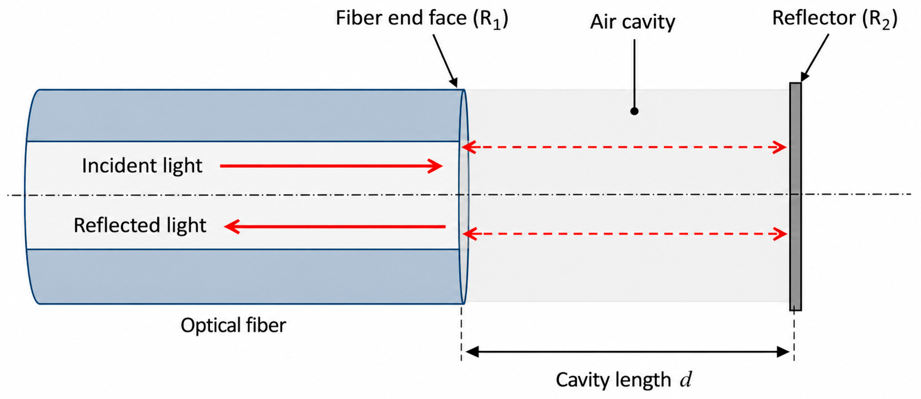
The sensing head comprises the cleaved end face of a single-mode fiber and a parallel external reflector, which form a low-finesse air cavity of length d (Figure 1). Light reflected at the fiber-air interface interferes with light returning from the reflector. When higher-order round trips are neglected, the reflected spectrum can be represented by the two-beam model used for low-finesse EFPI sensors [13,14,15,16]:

I_r(λ) = A(λ) + B(λ) cos [4πnd/λ + φ₀],

(1)

where I_r is the detected reflected intensity, A is the slowly varying background, B is the fringe envelope, n is the refractive index of the cavity medium (approximately unity for air), λ is the vacuum wavelength, and φ₀ collects constant reflection phase terms. Axial motion of the reflector changes d and therefore the spectral fringe frequency.

2.2. Cavity Length Demodulation and Strain Conversion

Adjacent minima at wavelengths λ_m and λ_m+1 satisfy successive interference orders. For a slowly varying refractive index, an initial estimate of the absolute cavity length is obtained from the local free spectral range as

d = λ_mλ_m+1/{2n[λ_m+1 − λ_m]}.

(2)

Because the wavelength span contains many fringes, the estimate is refined by removing the background, extracting and unwrapping the analytic-signal phase φ, and fitting phase against wavenumber k = 2π/λ. The slope gives

d = (1/2n)(dφ/dk),  k = 2π/λ.

(3)

Regression over the full scan uses more spectral samples than a two-minimum estimate and reduces sensitivity to the wavelength position of any single fringe. In the mechanical assembly, the fiber mount is fixed to the base while the reflector follows the moving end of the mortar prism. Taking compressive shrinkage as positive, the engineering strain is

ε(t) = −[d(t) − d₀]/L × 10⁶  (µε),

(4)

where d₀ is the reference cavity length and L = 250 mm is the mechanical gauge length. Thus, 2 nm of cavity shortening corresponds to 8 nε; the nominal conversion magnitude is 4 nε/nm. Equations (2) and (3) use the approximation that the air refractive index is constant over the scan. More generally, the phase slope measures the group optical length, with group index n_g = n − λ(dn/dλ); accurate environmental correction must use the index appropriate to the demodulation model. Changes in refractive index and differential thermal expansion can both be interpreted as strain if left uncompensated, as discussed in Section 5.2 and Section 5.3.

3. Materials and Methods

3.1. Mortar-Coupled Sensor Assembly

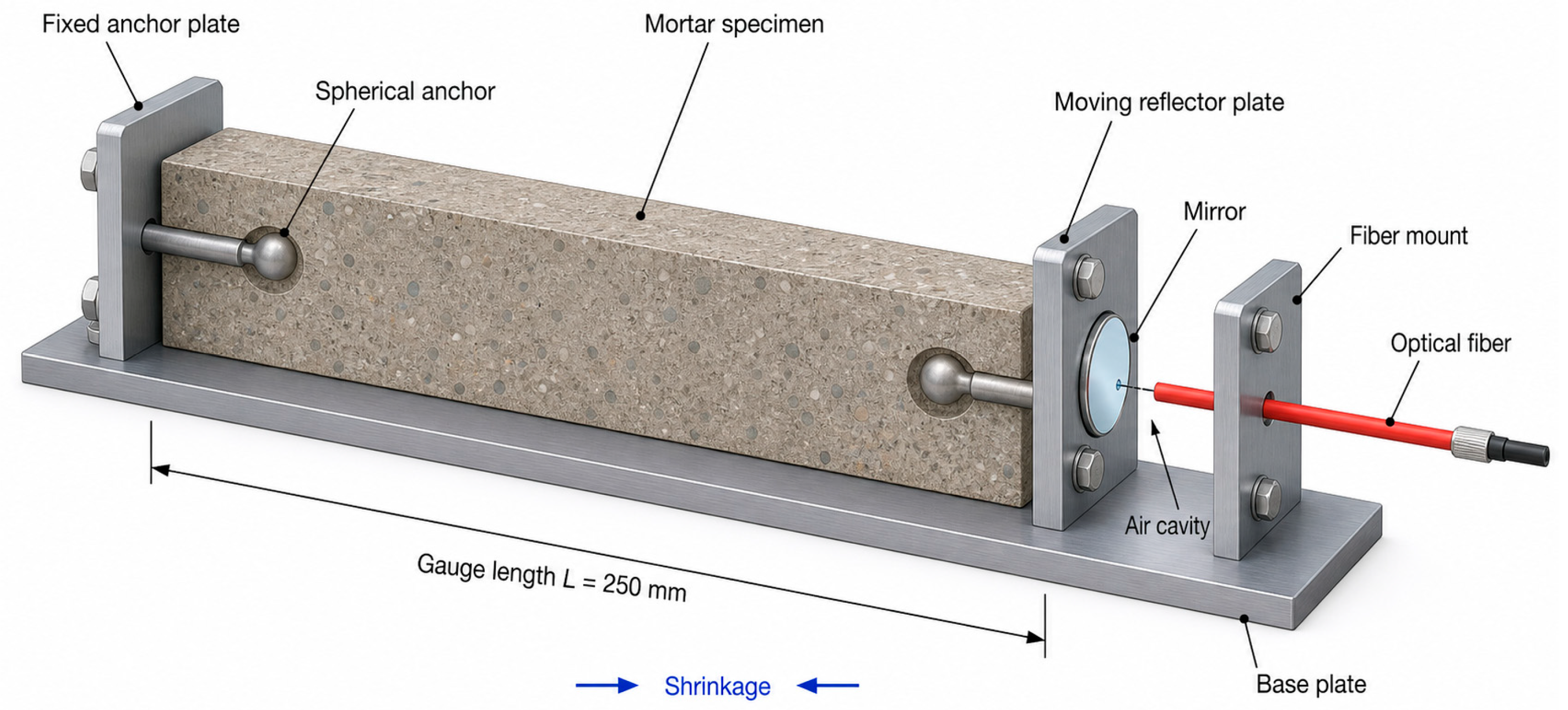
Figure 2 shows the 3D layout of the long-gauge sensor. The mortar prism measured 25 mm × 25 mm × 250 mm, and strain was measured along its 250 mm axis. A fixed anchor plate and a moving reflector plate were coupled to opposite ends of the specimen through rods terminating in spherical anchors. The enlarged spherical ends remained embedded after casting and limited end slip during shrinkage. The fixed anchor plate and the separate fiber mount were bolted to a rigid base. The moving plate carried a polished mirror aligned normal to the fiber axis; its axial displacement changed the air gap between the mirror and the cleaved fiber end.

To minimize restraint from the support, a polytetrafluoroethylene film coated with grease was placed between the specimen and the base before casting. After demolding, the prism was therefore mechanically coupled at its ends but free to slide relative to the base. This arrangement converts specimen shortening into reflector motion without requiring the optical fiber itself to be bonded along the mortar surface.

Three sensing assemblies with the same mechanical layout were used for the three mortar specimens. Reproduction of the layout requires control of the anchor spacing, fiber–mirror alignment, and freedom of the moving plate. In a repeatable assembly procedure, the anchors should be located with a gauge-setting jig during casting; after demolding, the cleaved fiber and mirror should be aligned to obtain stable spectral fringes, the initial cavity should be set within the interrogation range, and the zero and displacement response should be checked for each assembled head. The three operating assemblies demonstrate that the layout can be implemented more than once.

The present arrangement is a laboratory fixture, not a qualified field package. For practical use, a dust- and splash-resistant cover is recommended around the optical gap and mounts, with strain relief for the fiber lead. A compliant bellows or sliding cover should protect the moving reflector without appreciably restraining specimen shortening; its stiffness and friction must be checked after installation. Corrosion-resistant mounts and a protected optical compartment can reduce contamination and alignment changes. A dry sealed compartment or filtered vent could be evaluated for the optical gap, but pressure effects and the influence of any cover on specimen moisture exchange must be characterized.

3.2. Optical Interrogation and Data Acquisition

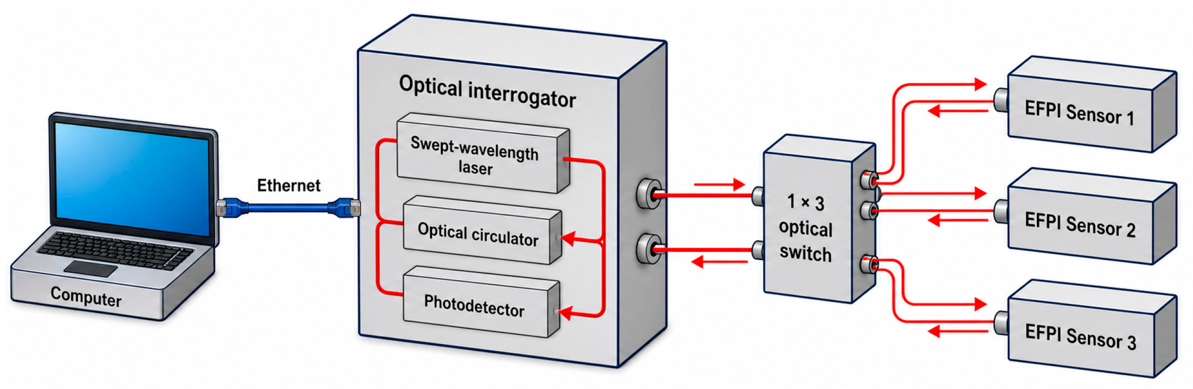
A swept-wavelength interrogator (SM125, Micron Optics, Atlanta, GA, USA) supplied light over 1510–1590 nm and detected the reflected EFPI spectrum. The interrogator contains a swept laser, optical circulator, and photodetector. A computer communicated with the instrument through Ethernet, acquired the spectra, calculated cavity length, displayed the real-time result, and stored the measurements. The acquisition–demodulation–storage cycle was 1 s. For three-specimen mortar monitoring, an optical switch addressed three EFPI channels sequentially, as illustrated in Figure 3.

3.3. Calibration and Stability Protocols

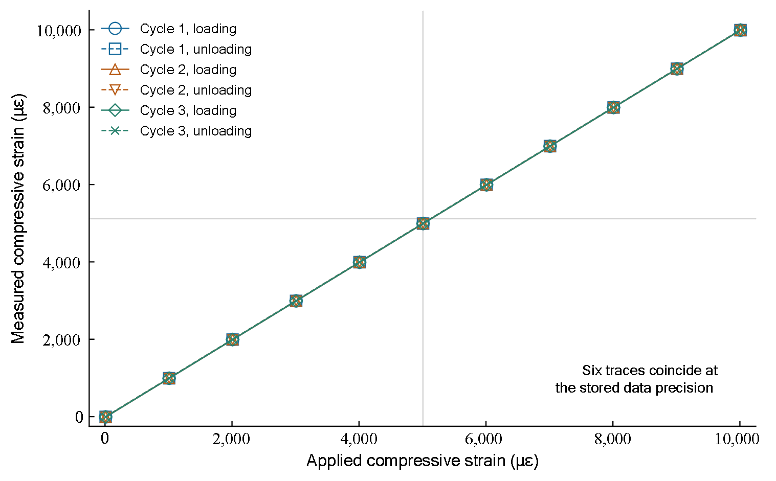
The reflector was driven by a displacement stage with a nominal 2 nm resolution. For the full-range test, a strain of 10,000 µε over the 250 mm gauge corresponds to a cavity length change of 2.5 mm. The commanded compressive strain was increased from zero to 10,000 µε in 1000 µε increments and then decreased in the same increments. Three loading–unloading cycles were recorded. At each set point, the spectrally demodulated cavity length was converted to strain using Equation (4) and compared with the stage command. These repeated calibration cycles assess the instrument response; they are not independent mortar shrinkage experiments.

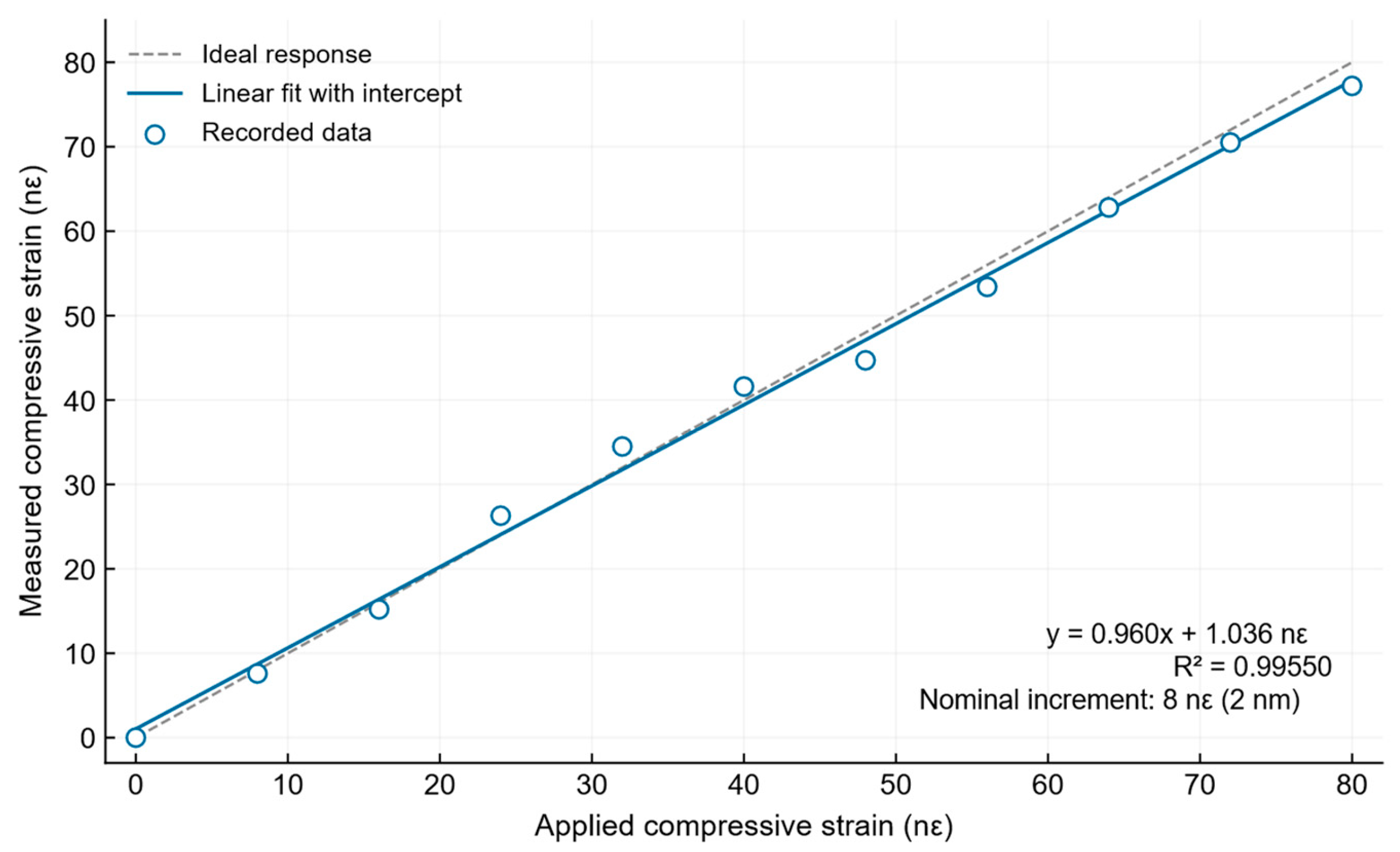
The incremental response was evaluated separately with 2 nm commanded displacement increments, equivalent to 8 nε over the 250 mm gauge. The 11 measured–applied strain pairs spanning 0–80 nε were fitted by ordinary least squares with a free intercept. For short-term stability, 100 consecutive readings were collected with the assembly in a chamber set to 20 °C. Only the series mean was removed; no smoothing or detrending was applied. The sample standard deviation was calculated as s_y = √[Σ(y_i − ȳ)²/(N − 1)], with N = 100. The input-referred noise-equivalent strain was estimated as ε_NE = s_y/|S|, where S is the local measured strain/applied strain slope. Because the output is already expressed as strain, S is a dimensionless calibration gain; the nominal cavity-to-strain conversion is not applied a second time.

3.4. Mortar Specimens and Shrinkage Monitoring

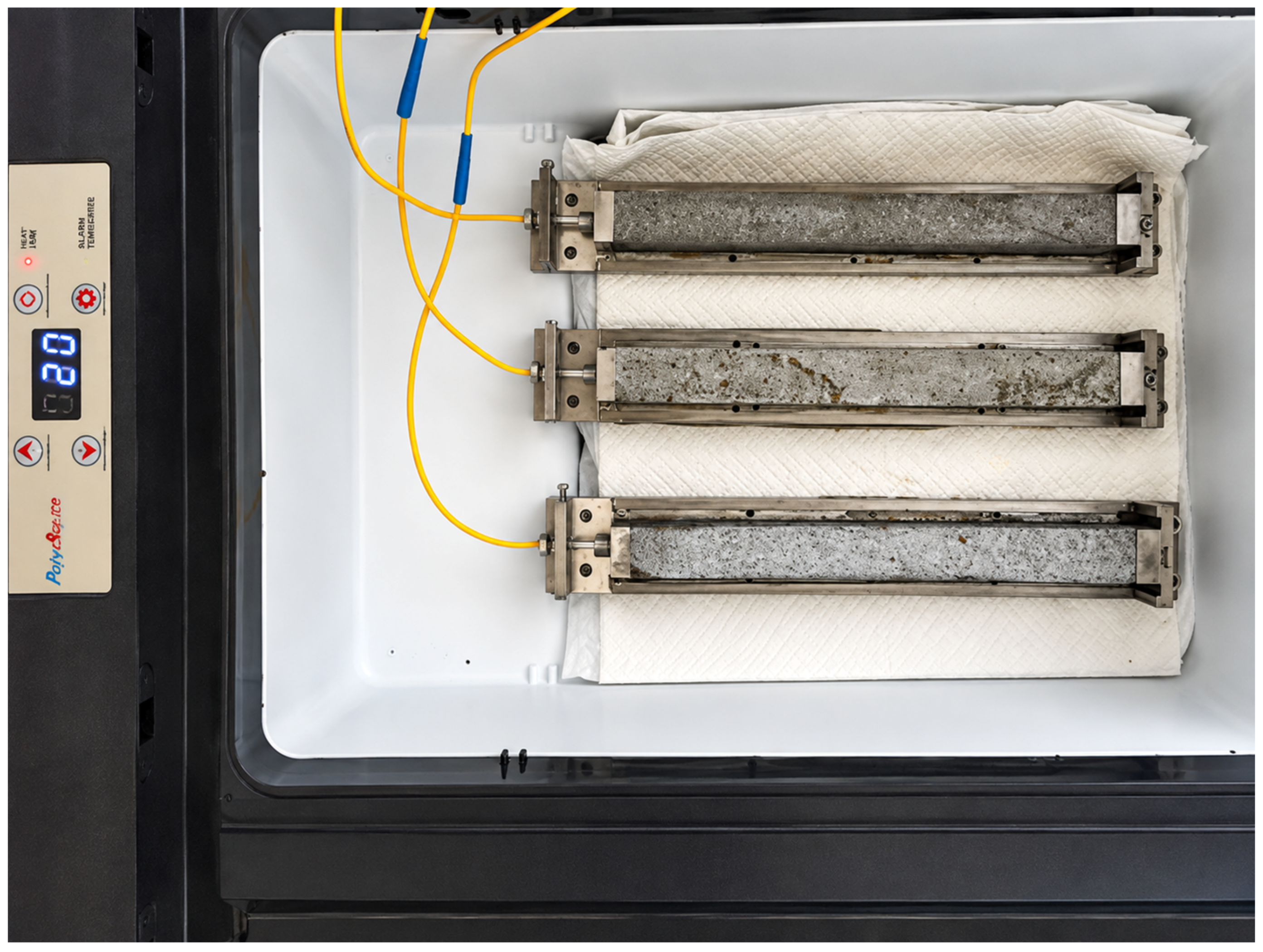
Three mortar mixtures were prepared using P.O 42.5 Portland cement and sand with a maximum particle size of 2.0 mm and a fineness modulus of 2.8. The water-to-cement ratios were 0.4, 0.5, and 0.6, with the other preparation steps kept consistent. One 25 mm × 25 mm × 250 mm prism was cast for each mixture (n = 1 per water-to-cement ratio; three specimens in total). The specimens were demolded after 24 h, the fibers and mirrors were installed, and the assemblies were placed in a chamber with a nominal setting of 20 ± 1 °C. The three optical channels were interrogated sequentially over a common 14-day monitoring period, with one stored value every 0.1 h. Monitoring time begins at the reference reading after installation; it is not the elapsed time since casting. No synchronized specimen temperature or relative humidity histories are available for this record, and no temperature or humidity correction is applied. The specimen arrangement is shown in Figure 4.

4. Results

4.1. Spectral Response and Full-Scale Calibration

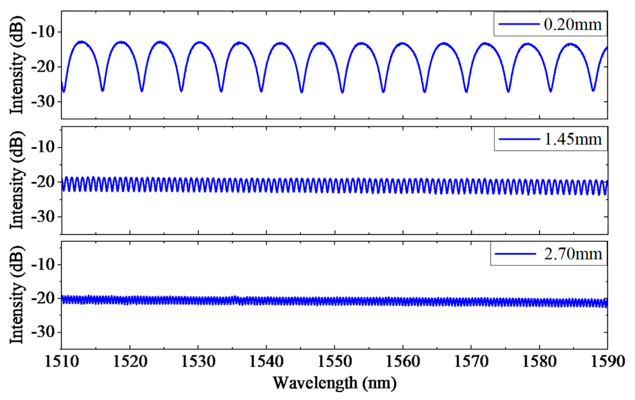
Representative spectra at cavity lengths of 2.70, 1.45, and 0.20 mm are shown in Figure 5. These values correspond to nominal compressive strains of 0, 5000, and 10,000 µε, respectively. As the cavity shortened, the number of fringes across the 1510–1590 nm scan decreased, consistent with the proportionality between spectral frequency and optical path length. The plotted envelope amplitude also increased at shorter cavity lengths, consistent with improved return-beam overlap.

Figure 6 presents the three loading–unloading cycles over the nominal 0–10,000 µε range. All six measured strain series coincide with the applied set points at the precision retained in the plotting data. This supports a near-unity response over the tested range.

4.2. Incremental Resolution and Short-Term Stability

Figure 7 shows the 11-point response to nominal 2 nm displacement increments. A linear fit with a free intercept gives y = 0.960x + 1.036 nε and R² = 0.99550, where x and y are applied and measured strain in nε. The 8 nε increments were distinguishable over the tested 0–80 nε interval. Relative to the 10,000 µε nominal range, this demonstrated increment is 8 × 10⁻⁷ of full scale. It is an incremental test result, not the noise-equivalent strain or a traceable uncertainty bound, because the commanded displacement step equals the nominal resolution of the reference stage.

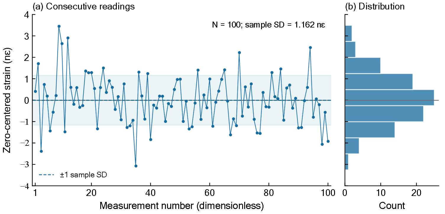
For the 100-reading stability record, the raw mean was 0.1231 nε, and the sample standard deviation was 1.162 nε. After mean removal, the observed range was −3.067 to +3.455 nε (Figure 8). Using the local gain S = 0.960 gives ε_NE = 1.162/0.960 ≈ 1.21 nε (1σ); the corresponding 3σ multiple is 3.63 nε. Before gain correction, the output standard deviation corresponds to 0.291 nm of cavity length fluctuation using the nominal 4 nε/nm conversion.

4.3. Fourteen-Day Mortar Shrinkage

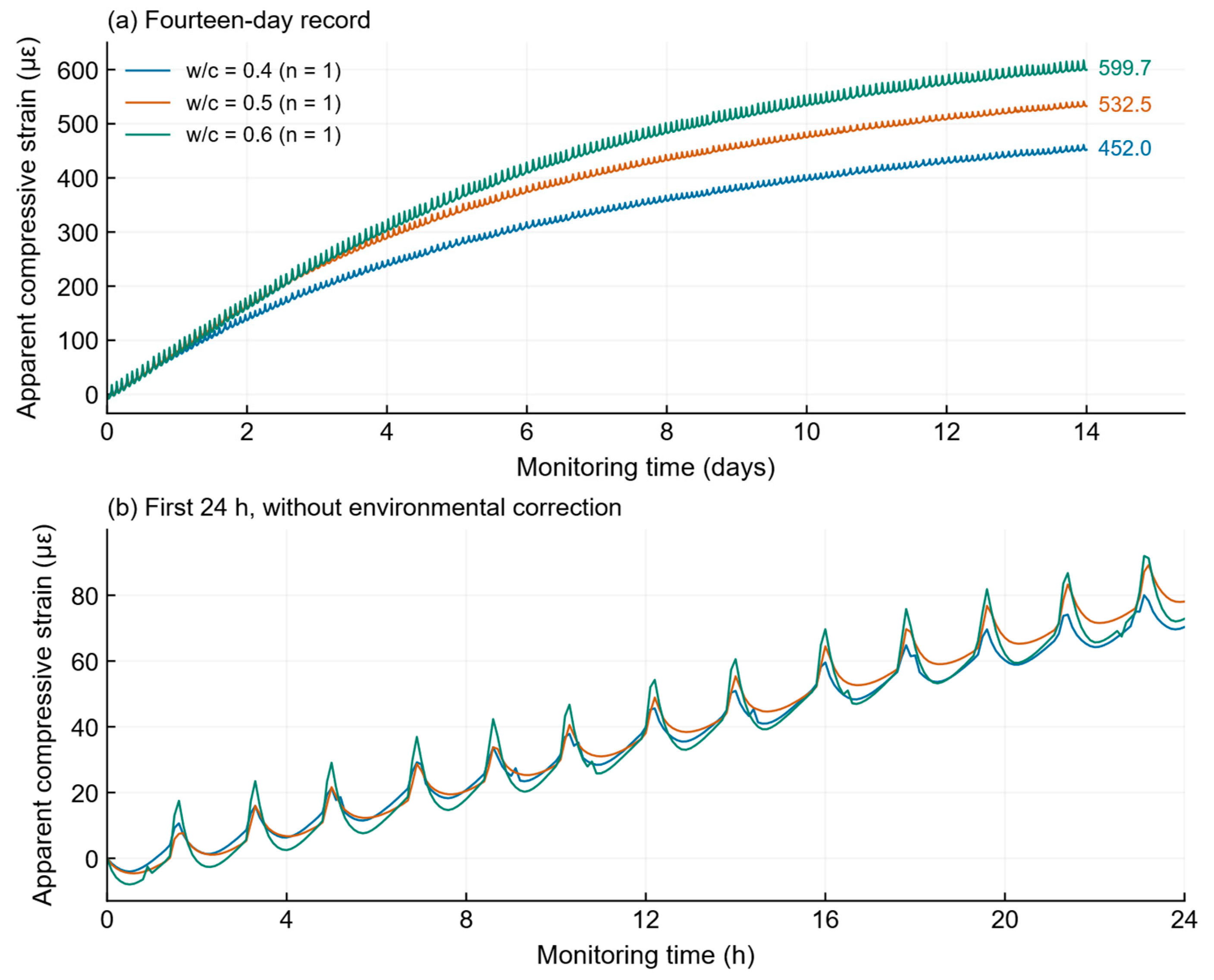
Figure 9 shows the recorded apparent compressive strain, with specimen shortening defined as positive. After the initial transient, each record shows an overall increase with a decreasing average rate. At 336 h (14 monitoring days), the values are 452.0 µε for a water-to-cement ratio of 0.4, 532.5 µε for 0.5, and 599.7 µε for 0.6, calculated from the final stored sample of each series. The ordering describes these three individual specimens and does not establish a statistically significant mixture effect. Figure 9b enlarges the first 24 h without filtering or environmental correction. Recurring excursions occur on an approximately two-hour scale. Chamber cycling and the coupled thermal response of the mortar and fixture are possible explanations.

5. Discussion

5.1. Interpretation of Resolution and Accuracy

The long mechanical gauge converts small displacements into small engineering strains: a 2 nm cavity change over 250 mm corresponds to 8 nε. The incremental response and the 1.21 nε input-referred noise estimate characterize different aspects of performance. The former is limited by the nominal stage increment, whereas the latter describes short-term dispersion referred through the measured local gain. Neither quantifies systematic effects from stage calibration, gauge length uncertainty, mounting, refractive index, or temperature. Comparisons with dynamic interferometers such as [18] must also account for bandwidth and averaging; the present time-domain standard deviation cannot be compared directly with noise amplitudes expressed per square root of hertz.

5.2. Temperature Sensitivity and Compensation

The sensor is not intrinsically temperature insensitive. Temperature can change the actual mortar length, expand the base and mounting components differentially, and alter the optical path through the air cavity. These effects can be interpreted as strain by Equation (4). A chamber setting of 20 ± 1 °C does not establish a negligible thermal contribution at the nanostrain scale. The 100-reading test at a 20 °C setting characterizes short-term output noise only; it is not a temperature sensitivity calibration.

A practical compensation procedure should measure temperature near each optical head and specimen and determine an effective thermal coefficient for the assembled system under a known mechanical condition. For an approximately linear and sufficiently uniform temperature change, an instrument correction can be written as ε_corr = ε_obs − C_T,inst ΔT, where C_T,inst is independently calibrated. Removal of the mortar’s real thermal deformation, when the desired measurand is nonthermal shrinkage, additionally requires an appropriate specimen thermal-expansion model. One chamber temperature channel or a coefficient borrowed from another package is not sufficient under thermal gradients. The reported monitoring record does not include a thermal sweep, an assembly coefficient, or synchronized temperature measurements; therefore, no numerical temperature compensation is claimed.

5.3. Airflow and Humidity Effects in the Cavity

The cavity responds to optical path length, not to geometric separation alone. At a fixed physical gap and for a small change in the effective refractive index, a demodulator using a fixed index n₀ gives an apparent gap change δd_app ≈ d δn/n₀. The magnitude of the corresponding strain error is approximately (d/L)|δn|/n₀ in dimensionless strain. For L = 250 mm and d = 0.20–2.70 mm, an illustrative index change of 10⁻⁶ would produce an apparent strain magnitude of approximately 0.8–10.8 nε. This is a sensitivity calculation, not an estimate of the actual environmental error in this experiment.

Air refractive index depends on temperature, pressure, humidity, wavelength, and gas composition [27]. Airflow is not a separate equilibrium index variable, but it can change local temperature, pressure, and humidity or introduce gradients and mechanical vibration. Humidity can therefore affect the optical readout as well as mortar moisture loss; condensation may additionally degrade the reflector signal. Protection of the optical gap can reduce direct air exchange and contamination, but neither sealing nor venting guarantees a constant optical path. Environmental measurements and an appropriate phase or group index model are needed to quantify the correction. Consequently, the cavity index contribution cannot be assumed negligible relative to the measured short-term noise.

5.4. Mortar Interpretation and Experimental Limitations

The larger final apparent strain in the higher-water-content specimen is compatible with moisture-dependent deformation mechanisms [21,22,23,24], but water-to-cement ratio is not the only possible explanation for the ordering. The 452.0–599.7 µε endpoints combine material deformation with fixture and environmental contributions. Relative humidity affects moisture exchange and drying, while temperature affects both material behavior and the sensing assembly. Without synchronized environmental measurements, humidity control information, or specimen mass loss records, the drying, autogenous, and thermal components cannot be separated. The excursions in Figure 9 must therefore not be assigned uniquely to chamber temperature cycling. The multiparameter and compensated approaches in [25,26] provide relevant directions for further validation.

One independently cast specimen was measured for each water-to-cement ratio. Repeated time samples and the three instrument-calibration cycles do not supply specimen-level replication; therefore, no between-specimen standard deviations, confidence intervals, or significance tests are reported. Independent batches and multiple specimens per mixture are needed to establish repeatability of the mortar histories. Further validation should combine synchronized specimen temperature, chamber relative humidity, and mass loss with an independently calibrated thermal response and a traceable displacement reference. Manufacturing variation, anchor slip, alignment retention, and protective-package performance also require repeated assembly and wetting–drying or thermal-cycle tests. These limitations restrict the current application to a feasibility demonstration.

6. Conclusions

A long-gauge EFPI sensor was developed to convert mortar end displacement into spectrally demodulated cavity length change. Loading–unloading measurements cover a nominal 0–10,000 µε range over a 250 mm gauge. A separate incremental test distinguishes nominal 8 nε steps, with a local fit slope of 0.960 and R² = 0.99550. The 100-reading stability record has a sample standard deviation of 1.162 nε, corresponding to an estimated input-referred noise-equivalent strain of 1.21 nε (1σ) under the tested short-term condition. The 14-day records reach apparent compressive strains of 452.0, 532.5, and 599.7 µε for the individual specimens with water-to-cement ratios of 0.4, 0.5, and 0.6, respectively. These results support continuous long-gauge monitoring.

References

1. Grattan, K.T.V.; Sun, T. Fiber optic sensor technology: An overview. Sens. Actuators A Phys. 2000, 82, 40–61. [Google Scholar] [CrossRef] [Scilit]
2. Lee, B. Review of the present status of optical fiber sensors. Opt. Fiber Technol. 2003, 9, 57–79. [Google Scholar] [CrossRef] [Scilit]
3. Culshaw, B.; Kersey, A. Fiber-optic sensing: A historical perspective. J. Light. Technol. 2008, 26, 1064–1078. [Google Scholar] [CrossRef] [Scilit]
4. Leung, C.K.Y.; Wan, K.T.; Inaudi, D.; Bao, X.; Habel, W.; Zhou, Z.; Ou, J.; Ghandehari, M.; Wu, H.C.; Imai, M. Review: Optical fiber sensors for civil engineering applications. Mater. Struct. 2015, 48, 871–906. [Google Scholar] [CrossRef] [Scilit]
5. López-Higuera, J.M.; Rodriguez Cobo, L.; Quintela Incera, A.; Cobo, A. Fiber optic sensors in structural health monitoring. J. Light. Technol. 2011, 29, 587–608. [Google Scholar] [CrossRef] [Scilit]
6. Wu, T.; Liu, G.; Fu, S.; Xing, F. Recent progress of fiber-optic sensors for the structural health monitoring of civil infrastructure. Sensors 2020, 20, 4517. [Google Scholar] [CrossRef] [Scilit] [PubMed]
7. Majumder, M.; Gangopadhyay, T.K.; Chakraborty, A.K.; Dasgupta, K.; Bhattacharya, D.K. Fibre Bragg gratings in structural health monitoring-Present status and applications. Sens. Actuators A Phys. 2008, 147, 150–164. [Google Scholar] [CrossRef] [Scilit]
8. Moyo, P.; Brownjohn, J.M.W.; Suresh, R.; Tjin, S.C. Development of fiber Bragg grating sensors for monitoring civil infrastructure. Eng. Struct. 2005, 27, 1828–1834. [Google Scholar] [CrossRef] [Scilit]
9. Bao, X.; Chen, L. Recent progress in distributed fiber optic sensors. Sensors 2012, 12, 8601–8639. [Google Scholar] [CrossRef] [Scilit] [PubMed]
10. Barrias, A.; Casas, J.R.; Villalba, S. A review of distributed optical fiber sensors for civil engineering applications. Sensors 2016, 16, 748. [Google Scholar] [CrossRef] [Scilit] [PubMed]
11. Murphy, K.A.; Gunther, M.F.; Vengsarkar, A.M.; Claus, R.O. Quadrature phase-shifted, extrinsic Fabry-Pérot optical fiber sensors. Opt. Lett. 1991, 16, 273–275. [Google Scholar] [CrossRef] [Scilit] [PubMed]
12. Belleville, C.; Duplain, G. White-light interferometric multimode fiber-optic strain sensor. Opt. Lett. 1993, 18, 78–80. [Google Scholar] [CrossRef] [Scilit] [PubMed]
13. Han, M.; Zhang, Y.; Shen, F.; Pickrell, G.R.; Wang, A. Signal-processing algorithm for white-light optical fiber extrinsic Fabry-Pérot interferometric sensors. Opt. Lett. 2004, 29, 1736–1738. [Google Scholar] [CrossRef] [Scilit] [PubMed]
14. Shen, F.; Wang, A. Frequency-estimation-based signal-processing algorithm for white-light optical fiber Fabry-Pérot interferometers. Appl. Opt. 2005, 44, 5206–5214. [Google Scholar] [CrossRef] [Scilit] [PubMed]
15. Jiang, Y. Fourier transform white-light interferometry for the measurement of fiber-optic extrinsic Fabry-Pérot interferometric sensors. IEEE Photonics Technol. Lett. 2008, 20, 75–77. [Google Scholar] [CrossRef] [Scilit]
16. Xie, J.; Wang, F.; Pan, Y.; Wang, J.; Hu, Z.; Hu, Y. High resolution signal-processing method for extrinsic Fabry-Pérot interferometric sensors. Opt. Fiber Technol. 2015, 22, 1–6. [Google Scholar] [CrossRef] [Scilit]
17. Ma, Z.; Cheng, S.; Kou, W.; Chen, H.; Wang, W.; Zhang, X.; Guo, T. Sensitivity-enhanced extrinsic Fabry-Pérot interferometric fiber-optic microcavity strain sensor. Sensors 2019, 19, 4097. [Google Scholar] [CrossRef] [Scilit] [PubMed]
18. Zhou, B.; Wang, W.; Bai, X.; Hu, J.; Chen, B.; Ye, L.; Song, K. Resolution-increased fiber-optic strain sensor with a large dynamic range driven by white light. Opt. Lett. 2024, 49, 1057–1060. [Google Scholar] [CrossRef] [Scilit] [PubMed]
19. Liu, L.; Qin, F.; Xu, Y.; Sun, L.; Wang, N.; Zhang, J.; Gong, K. All-metal packaged temperature compensation fiber optic Fabry-Pérot strain sensor for high-temperature liquid metal environments. Measurement 2025, 256, 118501. [Google Scholar] [CrossRef] [Scilit]
20. Shams, G.; Rivard, P.; Moradian, O. Tensile strength and failure behavior of rock-mortar interfaces: Direct and indirect measurements. J. Rock Mech. Geotech. Eng. 2024, 16, 41–55. [Google Scholar] [CrossRef] [Scilit]
21. Bissonnette, B.; Pierre, P.; Pigeon, M. Influence of key parameters on drying shrinkage of cementitious materials. Cem. Concr. Res. 1999, 29, 1655–1662. [Google Scholar] [CrossRef] [Scilit]
22. Tazawa, E.; Miyazawa, S. Influence of constituents and composition on autogenous shrinkage of cementitious materials. Mag. Concr. Res. 1997, 49, 15–22. [Google Scholar] [CrossRef] [Scilit]
23. Jensen, O.M.; Hansen, P.F. Influence of temperature on autogenous deformation and relative humidity change in hardening cement paste. Cem. Concr. Res. 1999, 29, 567–575. [Google Scholar] [CrossRef] [Scilit]
24. Lura, P.; Jensen, O.M.; van Breugel, K. Autogenous shrinkage in high-performance cement paste: An evaluation of basic mechanisms. Cem. Concr. Res. 2003, 33, 223–232. [Google Scholar] [CrossRef] [Scilit]
25. Souza, E.; Pinheiro, P.; Coutinho, F.; Dias, J.; Pilar, R.; Pontes, M.J.; Leal-Junior, A. Smart Concrete Using Optical Sensors Based on Bragg Gratings Embedded in a Cementitious Mixture: Cure Monitoring and Beam Test. Sensors 2024, 24, 7998. [Google Scholar] [CrossRef] [Scilit] [PubMed]
26. Weisbrich, M.; Messerer, D.; Holschemacher, K. Measurement of early age deformations in cement-based materials using distributed fiber optic sensors. Cem. Concr. Compos. 2026, 165, 106353. [Google Scholar] [CrossRef] [Scilit]
27. Stone, J.A.; Zimmerman, J.H. Index of Refraction of Air. National Institute of Standards and Technology. Available online: https://emtoolbox.nist.gov/Wavelength/Documentation.asp (accessed on 10 September 2026).
Figure 1. Operating principle of the low-finesse extrinsic Fabry–Pérot interferometric sensor.
Photonics 13 00876 g001
Figure 2. Three-dimensional layout of the mortar-coupled EFPI strain sensor and its 250 mm gauge length.
Photonics 13 00876 g002
Figure 3. Three-channel optical interrogation architecture used to connect the computer, swept-wavelength interrogator, optical switch, and three EFPI sensors.
Photonics 13 00876 g003
Figure 4. Mortar specimens with water-to-cement ratios of 0.4, 0.5, and 0.6 installed in the chamber before monitoring. One specimen was tested per mixture.
Photonics 13 00876 g004
Figure 5. Reflection spectra measured at cavity lengths of 2.70, 1.45, and 0.20 mm during full-range strain calibration.
Photonics 13 00876 g005
Figure 6. Measured versus applied compressive strain for three loading–unloading cycles.
Photonics 13 00876 g006
Figure 7. Incremental response to nominal 2 nm displacement steps, equivalent to 8 nε over the 250 mm gauge. Symbols show the 11 recorded pairs; the solid line is an ordinary least squares fit with a free intercept, and the dashed line is the ideal response.
Photonics 13 00876 g007
Figure 8. Short-term output noise for 100 consecutive readings at a chamber setting of 20 °C: (a) mean-subtracted strain versus measurement number, a dimensionless index; (b) the distribution of the same readings. The shaded band and dashed lines denote ±1 sample standard deviation (1.162 nε). Only mean removal was applied. The nominal acquisition cycle was 1 s.
Photonics 13 00876 g008
Figure 9. Apparent compressive strain of individual mortar prisms: (a) the full 14-day monitoring period; (b) the first 24 h. Each curve represents one specimen at the stated water-to-cement ratio (n = 1); no replicate-based error bars are available. The chamber setting was nominally 20 ± 1 °C. Labels in (a) give the final stored values in µε. Time is measured from the initial reference reading after installation.
Photonics 13 00876 g009
Disclaimer/Publisher’s Note: The statements, opinions and data contained in all publications are solely those of the individual author(s) and contributor(s) and not of MDPI and/or the editor(s). MDPI and/or the editor(s) disclaim responsibility for any injury to people or property resulting from any ideas, methods, instructions or products referred to in the content.