Analysis of Machine Learning Models for Predicting the Quality Factor and Received Power in Free Space Optical Communication Systems

Abstract

The study examines the application of machine learning algorithms (MLAs) to enhance free space optical (FSO) communication performance by predicting quality-factor (QF) from key system parameters. FSO technology has developed as a promising solution for front-haul links in 5G, beyond the 5G (B5G), and 6G transmission networks. Nevertheless, performance of an FSO communication link is limited by environmental challenges like weather conditions, attenuation and turbulence that can degrade signal quality and affect QF at the receiving end. Using the data collected through simulation analysis in OptiSystem, we trained several MLAs in order to analyze performance of this system through accurate prediction of the QF. Analysis shows that received power serves as an important parameter in translating the overall QF of the received signal. Furthermore, it is shown that the prediction accuracy of the tree-based approach such as random forest and gradient boosting ranges above 97% are reliant on channel conditions and the predicted parameter type.

1. Introduction

Mobile communication technologies from the first four generations mainly focused on the maximum amount of information a system can transmit, which is measure bits per second (bps). However, the exponential growth in handheld devices has introduced several other challenges in the form of variable network services, high bandwidth applications, system cardinality, and low latency. Consequently, the next generation of mobile networks have focused their design on three main services including enhanced mobile broadband communication (eMBB), massive machine-type communication (mMTC), and ultra-reliable low latency communications (URLLC) to accommodate the growing requirement for bandwidth and high-speed computing [1,2,3,4].

mMTC is primarily targeted to support widespread network of devices with diverse and varied communication needs. eMBB focuses on providing significantly higher data rates, improved capacity, and seamless connectivity, enabling new and enhanced applications that require fast, reliable, and high-bandwidth communication. URLLC is utilized to provide highly reliable, real-time communication with minimal delays. This feature of 5G is crucial for applications that require both extreme reliability (close to 99.999% uptime) and very low latency (1 ms or less).

Design and implementation of a communication network that is able to fulfill these service requirements presents a significant challenge and requires careful evaluation and comparison of various available options [5]. The first step to rectify these challenges was addressed by moving from the conventional distributed radio access network (D-RAN) architecture to a centralized radio access network (C-RAN). D-RAN, that was introduced as the first generation of RAN architecture, which houses both the baseband processing units (BBUs) and the radio heads (RHs) at the same cell site. Wireless signal transmission to the end user via RHs and D-RAN was handled, whereas BBUs were employed to manage the baseband computing. D-RAN offered relatively simple deployment of radio access networks along with localized control. However, it lacked the efficiency and flexibility of centralized architectures along with overall network efficiency in terms of performance and cost as compared to C-RAN [1,3,6].

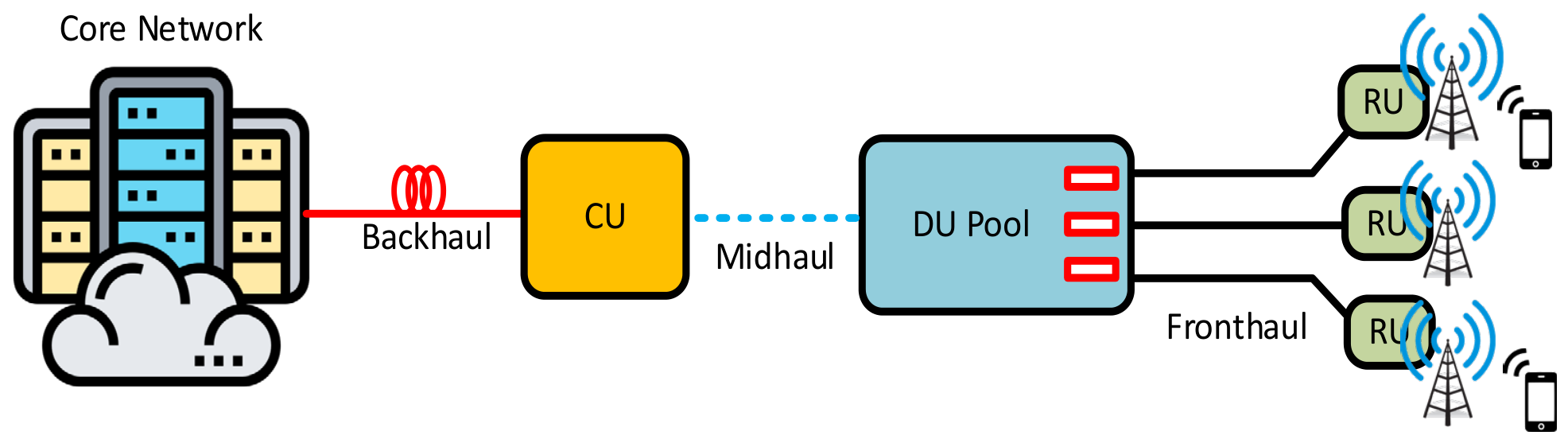
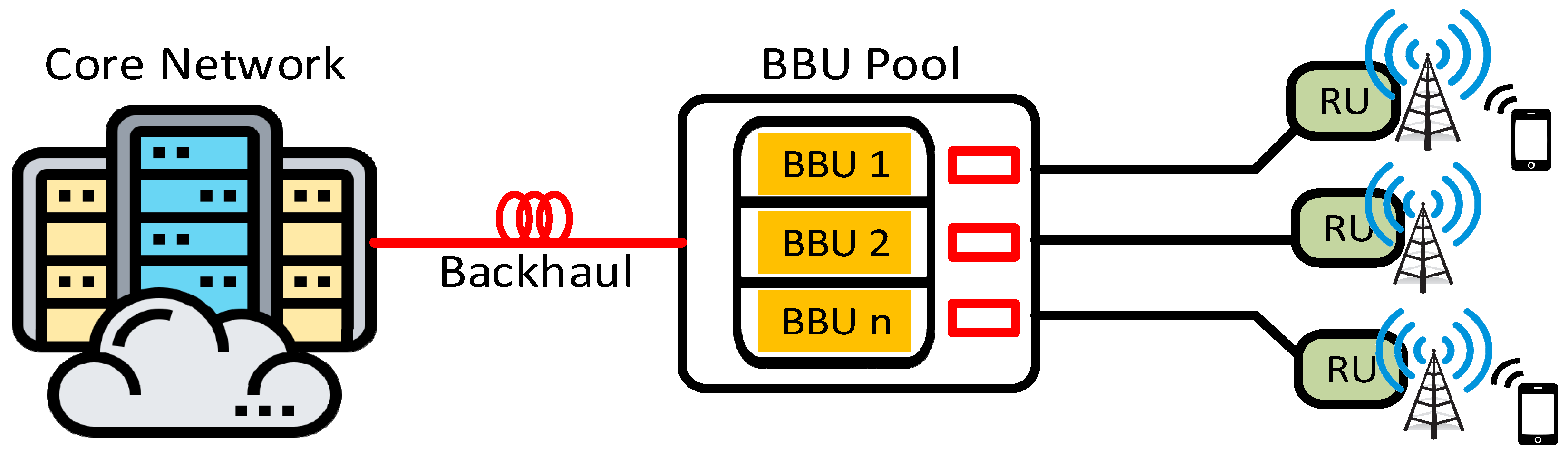
C-RAN, unlike D-RAN architecture, employs consolidated BBUs into a centralized BBU pool as shown in Figure 1. This BBU pool links to RHs spread across the coverage area via a high-capacity front-haul network and connects to the core network using a back-haul link. The adoption of C-RAN architecture introduced new enhancements and features for the network, increasing its flexibility and scalability to accommodate the growing needs of network users. For instance, sharing of a common pool of BBUs by multiple RHs can lead to better resource utilization, especially during low-traffic periods. Furthermore, network operators can save on hardware and operational expenses by centralizing BBUs in pool architecture. Fewer physical BBUs are needed that, in turn, reduces the overall cost on cooling, power consumption, and maintenance. In addition to the afore-mentioned advantages, centralization of BBUs allows for better coordination between cells, which can help with the mitigation of interference, especially in dense urban areas where cell overlap is common [1,2,3,4,5,6].

As shown in Figure 1, the C-RAN architecture centralizes baseband processing by pooling multiple BBUs at a single location, while lightweight radio heads (RHs) remain distributed at the cell sites. Each RH connects to the centralized BBU pool over a front-haul link, so baseband computation for many cell sites is consolidated rather than duplicated at every site as in D-RAN. This pooling is what enables the resource-sharing, cost, and interference-coordination benefits described above.

A proper solution for both 4G and 5G architectures has been proposed in the form of C-RAN. It has witnessed continuous development driven by the need to improve network performance and efficiency of network, in addition to reduce costs of deployment and operations. 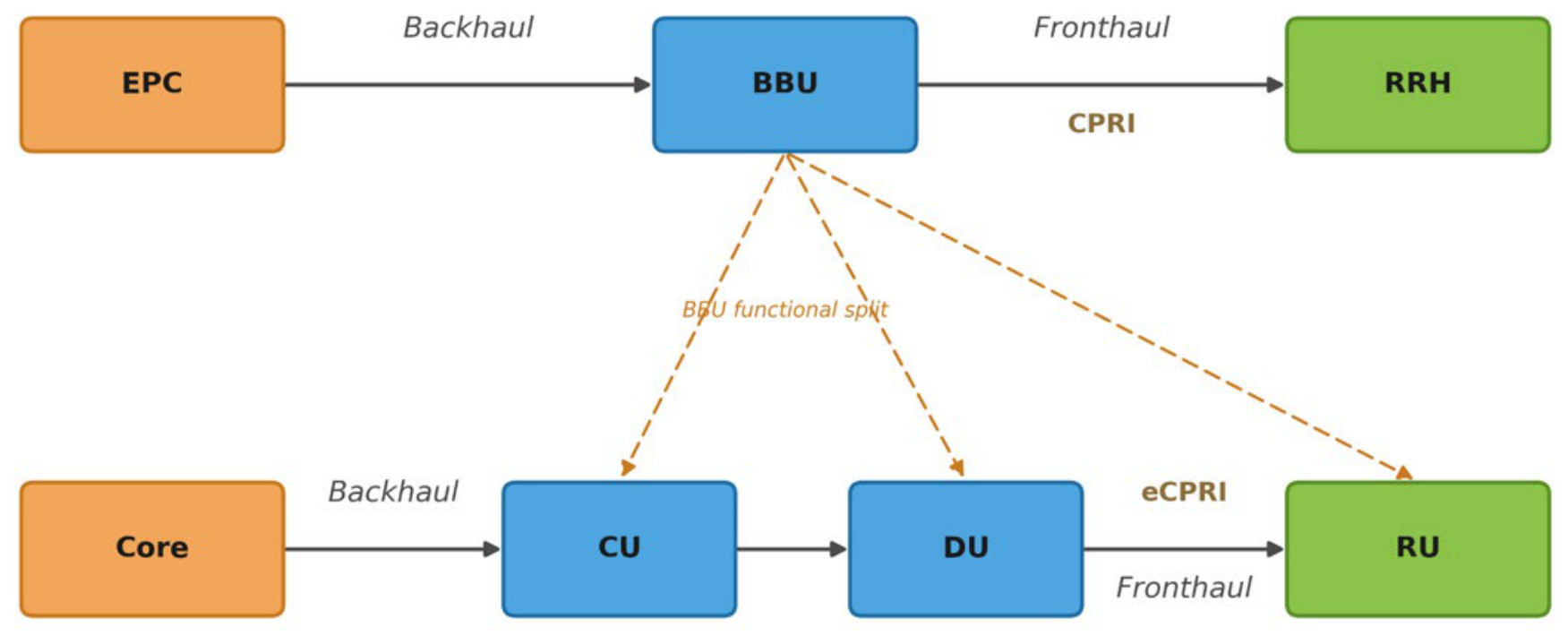Each evolution has brought new improvement and enhanced capacity to the network, making it more versatile, expandable, and adaptable for being utilized in beyond 5G and 6G architectures [3]. In the context of 6G, virtualized radio access networks (v-RAN) and open radio access networks (O-RAN), shown in Figure 2, tend to be favored more in comparison with the conventional C-RAN architecture because of their virtualized baseband processing, open-source nature, compatibility, agility, dynamic resource allocation, and rapid deployment [1,2,3].

Figure 2 illustrates the O-RAN architecture, in which the disaggregated CU, DU, and RU functions communicate over open, standardized interfaces rather than the vendor-proprietary interfaces typical of C-RAN. Baseband processing is virtualized and can run on commodity hardware, which allows RAN intelligent controllers and third-party applications to dynamically manage resource allocation, mobility, and interference across the network. This open, virtualized structure is what gives O-RAN its flexibility, multi-vendor interoperability, and rapid-deployment advantages over conventional C-RAN

The disaggregation of RAN functions, in C-RAN, v-RAN, and O-RAN, and partition of the network into different components has been made possible through the employment of different functional splits [2,3,6]. 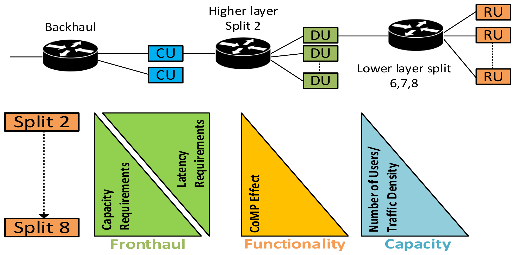Functional splits are primarily utilized to divide the RAN processing functions between different network units namely central unit (CU), the distributed unit (DU), and radio unit (RU) [1,2,3,4,5,6,7,8]. This allows for more flexible deployment, resource optimization, and, in the case of O-RAN, vendor interoperability through open interfaces. There are eight standardized split options as shown in Figure 4. These splits can be categorized into low-layer splits and high-layer splits, with the main difference being where in the protocol the split occurs, and which functions are centralized versus distributed as shown in Figure 3 [5,7,8].

Low-layer splits employ DU and RU to perform the processing functions that are closest to the physical layer. This ensures that the time-sensitive functions are performed locally, near the radio site, while allowing higher-layer functions to be centralized. On the other hand, high-layer splits utilize DU to handle low-layer physical processing, whereas higher level functions like mobility management and encryption place at the CU as shown in Figure 4. Both splits are further subdivided into eight categories depending on need and application of the network architecture. Both splits have their own advantages and disadvantages; however, low-layer splits have been favored more in comparison to their high-layer split counterparts [7,8].

As the functional splits between CU, DU, and RU move deeper into the protocol stack, the demand for high-speed data transmission dramatically increases on the front-haul (DU-RU link) and mid-haul (DU-CU link) section of the network [9,10]. For instance, at lower-layer splits, where time-sensitive tasks like modulation, coding, and MIMO processing are performed closer to the RU, the front-haul must handle massive amounts of real-time, partially processed data at very high speeds. On the other hand, at higher-layer splits, where more processing is centralized, the mid-haul connection must support the transfer of large volumes of raw or lightly processed data back to the CU.

Another primary obstacle towards implementation of an efficient front-haul link lies in the diverse and exponential growth of communication devices. Future networks like B5G and 6G are expected to witness a dramatic growth in communication devices like smartphones, tables, wearables devices, Internet-of-Things (IoTs), autonomous vehicles, smart meters, etc., each with unique characteristics and requirements [2,3,4,5,11]. Consequently, it is necessary to implement a robust front-haul infrastructure that can provide optimal performance, and seamless connectivity while adhering to the diverse traffic demands, bandwidth requirements, and latency constraints of each device to all types of devices [8].

In addition to the technical challenges, the cost of implementation for the densely deployed front-haul architecture is another significant factor that limits the practical implementation of RAN architecture in real-world applications [3]. A robust front-haul infrastructure can financially burden network operators and service providers, as it requires dense deployment of RUs in close proximity, which leads to high deployment and maintenance costs [12,13].

According to the ITU-T report, by 2030, 6G technology is expected to achieve peak data rates of 1 Tbps or higher, representing an increase of at least 50 times compared to 5G. Additionally, 6G will deliver latency of $\le$0.1 ms, which is at least 10 times lower than that of 5G across all conditions [11]. Furthermore, the amount of global data traffic and the number of devices connected to the network utilizing high-bandwidth and low-latency demanding applications is anticipated to grow exponentially during the next decade. Therefore, robust communication technology is required to provide an ultra-fast, high-capacity, low-latency, and a cost-effective transport network layer (TNL) connectivity between BBUs or DUs and the radio equipment (RRHs, RRUs, or RUs) near the subscribers’ domain [7,8].

In this context,

Table 1. Potential communication technologies and their specifications for next generation communication networks.

Technology	Throughput	Latency	Cost	Distance	Topology
P2P Fiber	1000 Gbps	Very low	High	100 km	P2P
PON	40 Gbps	Very low	Low	40 km	P2mP
xDSL	100 Mbps	Very High	Very low	500 m	P2P
FSO	10 Gbps	Very low	Low	5 km	P2P, P2mP
Microwave	1 Gbps	Moderate	Moderate	10 km	P2P, P2mP
mmWaves	10 Gbps	Moderate	High	1 km	P2P, P2mp

outlines potential communication technologies that are being explored to meet the high-capacity demands of future communication systems [1,4]. While microwave and mmWave links, already in use in wireless networks, offer a more affordable and faster deployment option compared to optical fiber solutions, their ability to support high data rates in large-scale systems, particularly in dense urban environments or advanced applications like ultra-reliable low-latency communications (URLLC), remains limited. Moreover, these technologies face significant transmission capacity constraints due to atmospheric attenuation, which becomes increasingly severe at higher mmWave frequencies, making them more vulnerable to weather conditions.

On the contrary, optical fiber technology like the passive optical network (PON), is widely recognized for its ability to provide high-capacity communication in terms of reach, data, and system cardinality. However, PONs require a large cost of deployment in both point-to-point (P2P) and point-to-multipoint (P2mP) implementation over an extended geographical area and dense urban environments.

Free space optical (FSO) is a transmission system that uses modulated light beams to send data over the atmosphere wirelessly between two fixed nodes. FSO communication technology has emerged as a viable alternative to optical fiber links, especially in scenarios where physical or cost constraints exist. Due to different functional splits and relaxing the front-haul capacity requirements, FSO becomes an attractive alternative for microwave and optical fiber in handling 5G and beyond front-haul data traffic s [14,15,16,17,18]. Apart from its performance benefits, FSO technology is economically viable due to the low deployment costs involved compared to using optical fibers. It does not involve civil works or trenching, which would have raised costs in terms of money and time. In addition, it uses the unlicensed optical window of operation of 800–1700 nm, meaning that there are no spectrum license fees needed for RF and mmWave technologies. FSO can be deployed in terrestrial environments for front-hauling and back-hauling, using point-to-point links from towers at cell sites to connect different radio units (RUs) to a centralized distributed unit (DU) pool, much like traditional microwave links [19].

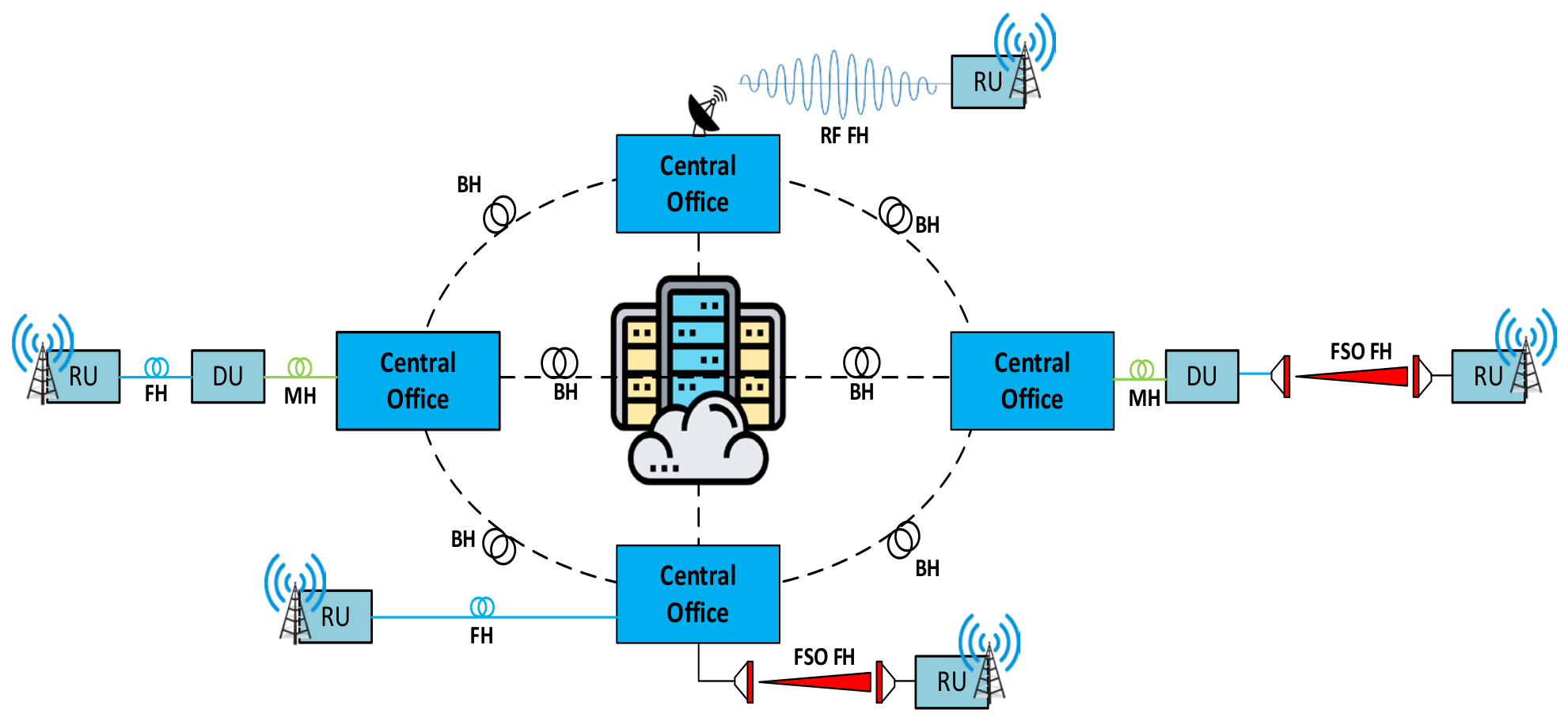
Figure 5 illustrates a fiber/wireless system within the C-RAN framework, in which the FH link can be implemented using a series of distinct technologies optical fiber links, radio link, radio-over-fiber (RoF), FSO, or even a combination of those [4]. The BH optical link serves a dual-purpose connecting COs to the core network and linking multiple COs to one another while DU can be implemented as an extension of the FH link. In this case, an MH link is used to connect CO to the DU.

However, several challenges exist with the deployment of FSO technology. A major concern is its vulnerability to environmental factors such as snow, clouds, heavy fog, and dust storms, all of which can attenuate the light signal and potentially disrupt the communication link. This can be attributed to the molecular/aerosol absorption and scattering of the propagating beam. Additionally, the scattering impact is closely connected to the size of the particles in relation to the optical signal’s wavelength, resulting in a random redistribution of signal energy. Consequently, various weather conditions demonstrate differing influences on the efficacy of the FSO communication system [18,19,20].

Another major constraint is atmospheric turbulence, atmospheric turbulence driven by local changes in heat and pressure creates tiny fluctuations in the air that end up distorting the beam. This turbulence leads to intensity fluctuations in the received signal, commonly referred to as the scintillation effect. As a result, there is a loss in signal-to-noise ratio (SNR) and the occurrence of signal fades. This directly impacts the system’s performance and reduces the effective operational range of the link because all of these effects contribute towards the degradation of received power which, in the worst-case scenario, can lead to link outages and an increase in the bit error rate (BER) [20].

Despite these challenges, FSO technology holds a notable advantage in its ability to support high data rates over long distances, outpacing the capacity of microwave and mmWave links. With thorough planning and carefully optimized system design, the adverse effects of weather and turbulence can be minimized, reinforcing FSO’s potential as a key component in future high-capacity communication networks [4].

Nevertheless, the FSO link is highly time-varying due to fluctuating outdoor environmental conditions such as fog, rain, and turbulence, which introduce channel impairments and reduces system’s performance in terms of reach, data, and the number of subscribers [16,20]. Efficient monitoring of channel conditions and required performance parameters is crucial that can facilitate dynamic adjustment of transmission parameters in response to varying environmental factors and improve overall capacity of the system.

In this context, machine learning (ML) offers powerful solutions for enhancing performance of the FSO systems. By leveraging data-driven models, ML can predict channel conditions in real-time, enabling dynamic adjustments in transmission parameters to optimize performance. For instance, ML algorithms can be trained to detect and predict variations in environmental factors, such as fog, rain, and turbulence, and their corresponding impact on signal quality factors (QF). This allows the system to proactively adjust transmission power, modulation schemes, or data rates to minimize bit error rate (BER) and maintain stable communication [17,18,19,20]. In this study, features like the distance between the optical beam and the PIN detector, path loss along the optical fiber, transmission power, diameters of antennas, data rate, and amplifier gain are fed into a machine learning algorithm to predict the received power at the receiver PIN photodiode. This predicted value of the received power is utilized to estimate the quality factor (QF).

Moreover, ML-based techniques can facilitate adaptive power detection, where power levels are continuously monitored and dynamically adjusted to compensate for sudden changes in atmospheric conditions. By implementing these adjustments, FSO systems can mitigate the adverse effects of signal degradation and maintain reliable data transmission [21,22,23]. Justification for the utilization of supervised learning in the current case study is provided by the existence of labeled training data that has been created artificially using simulated conditions in OptiSystem, whereby the input variables and their respective QF values have been identified. However, in instances whereby labeled training data is scarce, other machine learning algorithms can be used.

The contributions of the study can be highlighted in the following points:

• A simulation platform for multi-subscriber FSO-PONs in 5G front-haul applications is proposed;
• Received power and QF estimation through joint prediction via ML models;
• Comparison among four ML algorithms with an accuracy greater than 97%;
• Two-step feature selection approach involving random forest and Lasso regression;
• The scientific contribution of this study is not the machine learning algorithms themselves, which are established methods, but their joint application to simultaneously predict received power and QF from the same OptiSystem-generated feature set for a multi-subscriber FSO-PON front-haul scenario, combined with a two-step random forest/Lasso feature-selection pipeline that identifies received power as the dominant driver of QF under the simulated channel conditions. This link between an easily measurable physical-layer quantity (received power) and the harder to directly observe QF is what the proposed pipeline is intended to exploit for practical link monitoring.

2. Simulation Setup and Data Collection

FSO communication channel is highly susceptible to random and unpredictable variations due to changing turbulence conditions; therefore, it is crucial to collect extensive signal measurements under diverse scenarios. In the said reference, this study leverages OptiSystem, which is a powerful and a vastly recognized simulation tool for communication systems to analyzing and designing optical. OptiSystem is used to emulate outdoor channel conditions for a typical FSO communication link, allowing us to generate and collect data under numerous system parameters for training various machine learning models effectively.

The simulation setup is illustrated as Figure 6, which shows an FSO based PON for four subscribers. For a single BBU, the simulation model features a transmitter module that is formed by the combination of a pseudo-random bit sequence (PRBS) generator, non-return-to-zero (NRZ) module, Mach–Zehnder modulator (MZM), and laser diode (LD) array. PRBS generator is used to represent the BBU or CU that generates random data stream according to the system bit rate. Output of the PRBS is connected to a non-return-to-zero (NRZ) module, which encodes the binary data into an electrical signal for efficient transmission.

The encoded signal from the output port of the NRZ module is then fed into MZM that is used to the electrical signal into an optical signal while employing on–off keying (OOK). The modulator takes input from the PRBS generator at one port and connects to an LD on the second input port. A LD array is utilized in the simulation setup that is centered around the 1550 nm band.

The MZM end face is connected to a N-to-1 $(N:1)$ multiplexer where $N=4$ represents the total number of subscribers accessing the medium simultaneously. The multiplexed signal is then applied to an erbium-doped fiber amplifier (EDFA) module, which is incorporated to compensate for the signal degradation across the channel. The amplified signal at end-face of the EDFA is then fed to an FSO transmitter–receiver module, as shown in Figure 6.

Demultiplexer (De-MUX) is employed at the receiving end to recover the intended spectrum and forward it towards the corresponding ONT node that is installed at the RU. ONT module, for a single RU, houses a PIN photodiode that is utilized to convert the incoming signal from optical-to-electrical domain. The signal, in the electrical domain, is then fed to a low pass filter (LPF) that extracts the message signal and sends it towards the BER analyzer to obtain the required results. Optical power meters (OPM) are also employed to observe power at different points of the simulation network.

3. Simulation Parameters and Channel Model

In order to simulate a realistic scenario, this study utilizes the most commonly used system parameters across each component of the network.

Table 2. Simulation parameters for data collection.

Component Parameters	Value
LD linewidth	10 MHz
Transmission channel	1550 nm
Data per wavelength	10 Gbps
Transmitter nodes	16, 32, 48, 64
Bandwidth of multiplexer	10 GHz
Transmitter power	$10 \mathrm{d}\mathrm{B}$
Feeder fiber EDFA	$25 \mathrm{d}\mathrm{B}$
EDFA noise figure	4 dB
Photodiode responsivity	$0.8 \mathrm{A}/\mathrm{W}$
Sequence length	256 bits
Samples per bit	64
Signal format	NRZ
MUX filter bandwidth	10 GHz
Thermal noise	$7.5\times {10}^{-15}$ A2/Hz
Noise distribution	Gaussian
LPF cutoff frequency	$0.75 \times$Data rate

shows the system components simulation parameters that are utilized to collect the required data.

The system parameters chosen are in line with realistic FSO deployment scenarios. Because of its low ambient absorption and adherence to ITU-T optical communication standards, the wavelength of 1550 nm was selected. In order to provide realistic system modeling, a data rate of 10 Gbps per wavelength reflects typical 5G front-haul capacity requirements. Scalable multi-subscriber C-RAN installations with different traffic densities are represented by the transmitter node configurations (16, 32, 48, and 64). The photodiode responsivity of 0.8 A/W is consistent with standard PIN photodiode properties, and the transmitter power is chosen within typical FSO operating ranges documented in the literature [23]. The refractive index structural parameter is 10⁻¹⁵m^−2/3.

Several noise sources are taken into account in order to make sure that the system exhibits realistic behavior. Thermal noise is considered as described in Table 2. Shot noise is considered in the course of photodetection. Noise associated with the amplified spontaneous emission (ASE) generated by EDFA is considered in terms of a noise figure of 4 dB. RIN is not considered here to simplify the problem, and hence there might be some error in calculations at high optical power levels.

The FSO channel is configured with Gamma–Gamma (GG) model in order to assess the effect of channel irregularities on performance of the system. The GG model is a versatile approach that can be applied across a wide spectrum of turbulence, spanning from weak to strong turbulence regimes. The normalized light intensity is calculated by the model by utilizing small alpha $\left(\alpha \right)$ and large beta $\left(\beta \right)$ fluctuators, $I$ in order to include the effects of channels turbulence on overall performance of the system [14,21,22]. Distribution probability of $I$, in terms of $\alpha$ and $\beta$ can be written as [16,24]. The simulated results for received power and BER are consistent with trends reported in existing FSO studies [20,24], providing indirect validation of the adopted channel model.

There are several channel models employed in modeling atmospheric turbulence in optical wireless communication. Log-normal channel models can only be applied in the case of weak turbulence conditions while the negative exponential channel models can only be used in the case of strong saturated atmospheric turbulence conditions. However, real-life FSO communications experience medium or high turbulence conditions. In that regard, the Gamma–Gamma channel models are utilized in this work because they address small- and large-scale atmospheric turbulence conditions:

$$p\left(I\right)={\displaystyle \frac{2{\left(\alpha \beta \right)}^{\frac{\alpha +\beta }{2}}}{\Gamma \left(\alpha \right)\Gamma \left(\beta \right)}}{I}^{\frac{\alpha +\beta }{2}-1}{K}_{\alpha -\beta }(2\sqrt{\alpha \beta I})$$

(1)

where $k_{\alpha -\beta }(.)$ in Equation (1) shows the modified Bessel function, and $\Gamma \left(.\right)$ is the Gamma function as per the propagation distance d and now the values of $\alpha$ and $\beta$, which are the large-scale and small-scale eddies of the scattering process and can be expressed as:

$$\alpha ={\left[exp\left({\displaystyle \frac{0.49{\sigma }_l^2}{{\left(1+1.11{\sigma }_l^{2.4}\right)}^{1.17}}}\right)-1\right]}^{-1}$$

(2)

$$\beta ={\left[exp\left({\displaystyle \frac{0.519{\sigma }_l^2}{{\left(1+0.69{\sigma }_l^{2.4}\right)}^{0.833}}}\right)-1\right]}^{-1}$$

(3)

The different link atmospheric turbulence regimes are distinguished by the value of Rytov variance from Equations (2) and (3). The initial analysis includes the impact of the FSO link on received power (dBm) and BER at each RU module over a Gamma–Gamma channel and the index of refraction for the FSO structure is set to ${10}^{-15}{\mathrm{m}}^{-\frac{2}{3}}$ for the analysis in order to incorporate the effect of a moderately turbulent environment.

Table 3. FSO system parameters.

Simulation Parameter	Value (dB/km)
Channel	Gamma–Gamma
Index of refraction	${10}^{-15}{\mathrm{m}}^{-\frac{2}{3}}$
Range	Variable
Beam divergence	2 mrad
FSO transmitter aperture	5 cm
FSO receiver aperture	20 cm
Post channel EDFA	25 dB

shows that FSO system parameters and channel characteristics are utilized for simulation analysis.

The Gamma–Gamma channel model is chosen because it can efficiently simulate the impact of turbulence at different levels from weak to strong. While the log-normal model is applicable only at weak turbulence and the negative exponential model works at strong turbulence conditions, the Gamma–Gamma model considers both small- and large-scale fluctuations in irradiance via the shaping parameters. This makes it more suitable for realistic outdoor FSO scenarios [14,21,22]. Atmospheric conditions based on their respective attenuation coefficients in dB/km are also considered while collecting data for training different ML models. The attenuation coefficient quantifies the loss of signal strength per unit distance due to the scattering and absorption effects of different atmospheric phenomena. These values are crucial for designing and evaluating FSO communication systems, as atmospheric attenuation can significantly impact signal quality and system reliability.

Table 4. Channel attenuation values.

Weather Condition	Attenuation
Clear air	0.43–0.6
Light haze	1–1.2
Haze	3.1–4.6
Light rain	6.27
Moderate rain	9.64
Light fog	6.6–18.3

shows channel attenuation values that are utilized during the simulation analysis.

Attenuation coefficients related to various weather conditions have been chosen using standard atmospheric propagation models and experimental results found in the FSO communication literature.

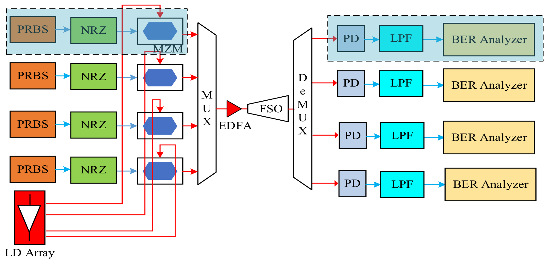
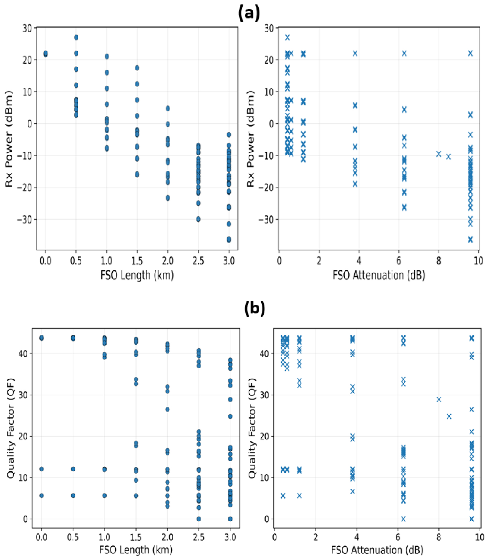
Data collection is performed by running multiple instances of the simulation model at different performance parameters while observing power received before the signal is fed to PIN photodiode and associated quality factor (QF). Figure 7 shows the results obtained for the simulation instance at 32 BBU nodes each communicating at 5 Gbps of data. The length of the FSO channel, channel attenuation, transmitter, and receiver powers are varied throughout the simulation to obtain different possible values of received power and associated QF.

4. Feature Extraction

This study sets out to explore predicting QF of the FSO communication links under varying channel conditions using different ML models. Consequently, it is of primary importance to select relevant features (system parameters) based on their ability to capture information related to the signal quality and associated power received at the ONT module.

In the quest to perform comprehensive analysis using ML models, this study considers multiple simulation parameters as features including data rate per BBU, transmitted power (Tx Power), FSO link length, FSO channel attenuation, transmitter aperture size, receiver aperture size, receiver amplifier gain, received power, and photodetector responsivity. Each of these features plays a critical role in determining the overall system performance. For instance, data rate and Tx power directly influence the signal’s strength and bandwidth requirements, while FSO channel length and FSO attenuation determine the path loss and signal degradation over different distances and atmospheric conditions.

Furthermore, received power is a crucial feature, as it provides direct insight into the strength of the signal after considering all transmission losses and gains. Receiver amplifiers gain and transmitter amplifications are also considered for the analysis. Both parameters are utilized throughout the analysis to adjust the received power for an acceptable value of QF at different data rates, channel lengths, and attenuation factors, respectively.

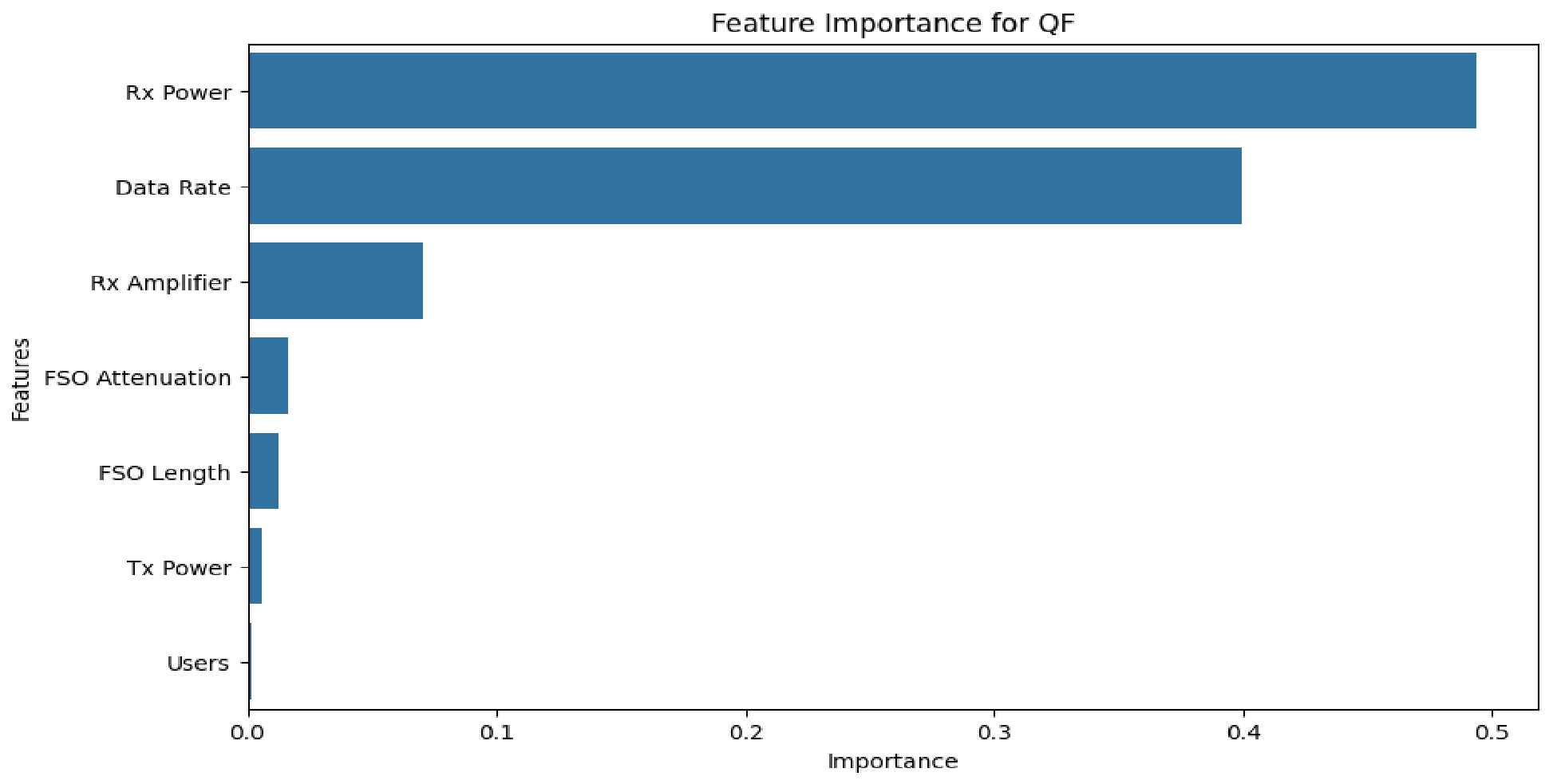
Figure 8 illustrates the importance of various features on QF of the FSO-based communication system. The goal is to understand which features are more powerful for monitoring QF of the FSO communication system. Random forest is utilized to select the most appropriate features and an ensemble learning approach. The random forest constructs multiple decision trees and aggregates their predictions for classification or regression. It also provides a measure of feature importance, making it useful for feature selection [20,23,25,26,27].

From the analysis, it is evident that the most influential feature impacting the QF is the received power at the PIN photodiode. This suggests that optimizing and controlling the received power significantly enhances the overall system performance. Other notable features include the data rate and receiver amplifier, which also contribute to the QF. Thus, focusing on these critical parameters can lead to substantial improvements in system efficiency and reliability.

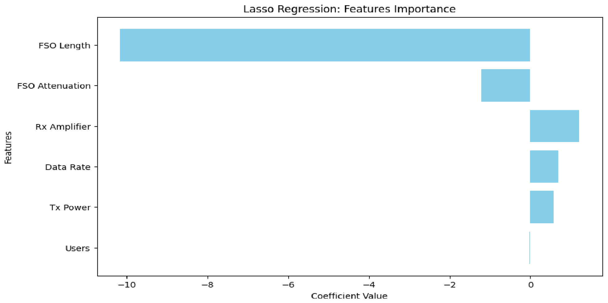
For further analysis, Lasso regression is performed to determine the features that impact received power at the PIN photodiode [27]. It can be observed that several features contribute to the variations in power received at the PIN photodiode. Among these, FSO length shows the strongest negative influence, indicating that increasing the FSO link length significantly reduces the Rx power as shown in Figure 9. FSO attenuation also exhibits a negative impact, emphasizing the importance of minimizing attenuation to maintain higher received power levels. However, these parameters are associated with channel properties and cannot be varied for general effectiveness of the system.

5. Dataset Characteristics

The dataset used for this study comprises 1120 samples with 11 features obtained from comprehensive simulation using OptiSystem. These samples have been divided based on different atmospheric conditions such as clear air, haze, rain, and fog, as indicated in Table 4 below. Stratified splitting into training and testing sets, performed at the ratio of 80:20, respectively, ensures that various channel conditions are proportionately represented in the split datasets. No balance method like oversampling or SMOTE has been utilized since there is an acceptable data distribution among different conditions.

A dataset of 1120 samples was considered adequate for this study for three reasons. First, the input space is comparatively low-dimensional (11 features), which keeps the samples-to-feature ratio (~100:1) well above commonly cited rules of thumb for classical and tree-based regressors. Second, the data were generated through a controlled, systematically varied simulation sweep rather than noisy field measurements, so the effective diversity of operating conditions per sample is higher than an equivalent-sized empirical dataset would provide. Third, model stability was verified independently of dataset size through 5-fold cross-validation (Section 6), which showed consistent R² performance across folds, indicating that the models are not overfitting to a particular train/test split. We acknowledge that expanding the dataset with additional turbulence and hardware-impairment scenarios remains a valuable direction for future work.

Analysis comparison between the feature importance scores using random forest algorithm and the coefficient scores of Lasso regression model indicates that both techniques exhibit a uniform trend in finding the most significant features. Both techniques show the importance of the received power and FSO link length features to have an impact on the performance of the system.

6. Models Implementation and Analysis

Machine learning algorithms (MLAs) are implemented in this paper using Python, and performance is analyzed using coefficient of determination $\left(R^2\right)$, and comparison of the actual versus predicted values [27,28,29]. Splitting of the data into train and test datasets is performed at the ratio of 80:20. For feature selection, methods like random forest feature importance and Lasso regression are used only on the train dataset to avoid any data leakage. Mathematically the coefficient of determination can be written as:

$$R^2=1-{\displaystyle \frac{MSE}{SST}}$$

(4)

Here, MSE represents the mean squared error, which measures how well a model explains the variance of the data and MSE calculates the average squared difference between the actual and predicted values, showing the magnitude of errors made by the model. Mathematically, MSE can be expressed as:

$$MSE={\displaystyle \frac{1}{n}}{\sum }_{i=1}^n{\left(y_i-\widehat{y_l}\right)}^2$$

(5)

where $n$ represents the total number of samples, and $y_i$ and $\widehat{y_l}$ are used to represent the true and predicted value of the variables, respectively. SST in $R^2$ gives the total sum of squares and can be expressed mathematically as:

$$SST={\sum }_{i=1}^n{\left(y_i-{\mu }_y\right)}^2$$

(6)

where, ${\mu }_y$ is used to give information about the sample meaning of features utilized in the analysis.

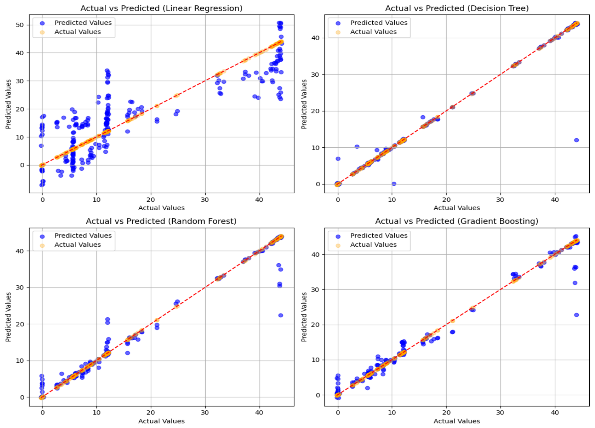
Figure 10 shows a comparison of four different MLAs, namely linear regression, decision tree, random forest, and gradient boosting for accurately predicting QF while utilizing multiple features from a dataset of 1120 × 11 features. Each scatter-plot displays predicted values versus actual values, with a red dashed line indicating the ideal prediction (where predicted values perfectly match the actual ones) [27,28,29,30].

It can be observed that predictions of the linear regression algorithm are somewhat scattered, indicating lower accuracy and larger errors for certain points. This can be attributed to the fact that linear regression models the relationship between dependent, QF, and independent variables as a linear equation $\left(Y={\beta }_0+B_1{X}_1+B_2{X}_2+\cdots +B_n{X}_n\right)$, which minimizes the sum of squared residuals (differences between actual and predicted values) to estimate the coefficients.

For predicting the values of QF at different input features, decision tree, random forest, and gradient boosting algorithms perform significantly better, with predictions closely aligning along the 45-degree line, showing high accuracy. Random forest (RF) and gradient boosting (GB) perform exceptionally well, indicating their suitability for this task. This is because random forest is an ensemble of decision trees. For each tree, the algorithm uses a random subset of data (bootstrap sampling) and randomly selects a subset of features. Predictions are averaged over all trees:

$$\widehat{y}={\displaystyle \frac{1}{N}}{\sum }_{i=1}^{N}Tre{e}_i\left(X\right)$$

(7)

where, $N$ represents the total number of decision trees in the RF model, and $X$ represents the input features for a data point at which we want to predict the target value $\widehat{y}$. $\widehat{y}$ is the average prediction across all trees in the ensemble, that helps in reducing variance and improving generalization.

On the other hand, GB operates by iteratively building the tree, with each subsequent tree learning from the residuals of the previous one. It minimizes a differentiable loss function $L\left(y,\widehat{y}\right)$ by adding new trees that predict residuals. Mathematically, the process can be expressed as:

$${\widehat{y}}_{m+1}={\widehat{y}}_m+\mathsf{ƞ}{f}_m\left(x\right)$$

(8)

where, $\mathsf{ƞ}$ is used to represent the learning rate of GB algorithm, whereas $f_m\left(x\right)$ gives the $m-th$ tree trained on the residuals. The iterative improvement utilized in GB algorithm makes it highly effective in fitting complex data patterns. In summary, the algorithms’ performance reflects their ability to model complex relationships. While linear regression lacks flexibility, ensemble methods like random forest and gradient boosting capture nonlinearity and interactions more effectively, leading to higher accuracy in predicting QF.

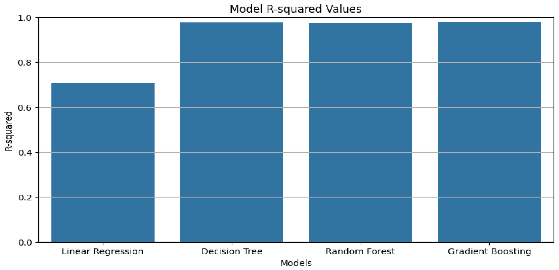
For further analysis, the R-squared values for the four MLAs are presented as a measure of each model’s effectiveness in predicting the QF for an FSO-based communication system. The R-squared value in Figure 11 indicates how well each model’s predictions align with actual data, with higher values indicating better performance. It can be observed that, decision tree, random forest, and gradient boosting show near-perfect R-squared values (close to 1.0), suggesting they capture the relationships between features and QF very effectively. These algorithms are more capable of handling complex, nonlinear interactions among features, which are common in FSO systems where factors like atmospheric turbulence, misalignment, and geometric path loss can nonlinearly impact QF. The simulations and training process were performed using Python 3.x through the use of the scikit-learn library. All the simulations were performed using a machine with Intel Core i7 CPU and 16 GB RAM. Training for each model took a relatively short amount of time, with the decision tree taking less than a second, but ensemble techniques such as gradient boosting taking around 3–5 s.

Linear regression, with a lower R-squared, performs comparatively worse due to its limitation to linear relationships. FSO communication systems are inherently complex, and linear models may not capture the intricate dependencies between variables that influence QF as effectively as tree-based ensemble methods.

k-fold cross-validation (where k = 5) was used for further evaluation of the model. This proves that the model has consistent R² values, suggesting that the model generalizes well and is not influenced by any train/test partitioning. Ensemble models perform better than linear regression models since they can capture nonlinear relationships that exist within the atmosphere channels.

While R² indicates how well each model explains overall variance, it does not by itself convey the typical magnitude of prediction error.

Table 5. Test-set error metrics for the four MLAs (QF prediction).

Model	MAE	RMSE	R2
Linear Regression	6.7718	8.0967	0.7447
Decision Tree	1.3344	3.9573	0.9390
Random Forest	1.3847	3.2837	0.9580
Gradient Boosting	1.3695	3.1964	0.9602

, therefore, reports mean absolute error (MAE) and root mean squared error (RMSE), alongside R², for all four MLAs on the held-out test set, to give a more complete comparative picture of model performance.

7. Model Interpretability

Model transparency can be improved by examining the feature importance of the top-performing model (gradient boosting). It is clear from the results that received power is the most important feature, with second and third place going to FSO link length and channel attenuation, respectively, which is in agreement with the random forest feature importance demonstrated in Figure 8. While SHAP analysis has not been carried out in this study, it is recommended for future research to obtain a clearer idea about how different features contribute to the model’s performance.

It is also worth noting the likely impact of factors not varied in this study. A turbulence coherence time shorter than the update rate of an adaptive prediction or compensation loop would limit the system’s ability to track rapid channel fluctuations, so ensuring the ML model’s inference rate stays ahead of the coherence time is important for real-time deployment. Pointing/alignment error introduces an additional geometric loss term not captured by the Gamma–Gamma model used here and would be expected to further reduce received power and QF at longer link distances, in a manner correlated with but distinct from turbulence-induced fading. Device nonlinearity, primarily from the MZM and EDFA operating near saturation, can distort the signal in ways that are not purely additive, which may reduce the accuracy of models trained only on data from the linear operating regime. Quantifying these effects through additional simulation sweeps or experimental validation is left for future work.

8. Conclusions

The exponential growth in internet traffic and the proliferation of new devices in networks demand innovative solutions beyond conventional modifications to communication systems. In this context, the present study investigates the potential of machine learning algorithms (MLAs) to enhance the quality factor (QF) in free space optics (FSO)-based optical communication networks. Data for this study were generated by simulating multiple FSO-based optical communication networks in OptiSystem. Feature selection was conducted using the random forest regressor and Lasso regression to identify the most influential factors for improving the QF of the received signal. The analysis revealed that the received power at the optical network terminal (ONT) module is the most impactful feature influencing QF at the receiving end. However, despite the favorable outcomes obtained, there are certain limitations with this research. First, the data collection process relies solely on simulations and lacks experimental testing in a practical environment of an FSO communication channel. Second, only the Gamma–Gamma channel model was examined, and no account was taken for changes in environmental conditions within the same period of time. Also, all of the data models are independent observations of the system. Finally, the research was performed using one particular setting only.

Subsequently, the study compares the predictive performance of four MLAs—linear regression, decision tree, random forest, and gradient boosting for estimating the received power at the ONT module under specific weather conditions. The results demonstrate that ensemble techniques like random forest and gradient boosting outperform linear regression and decision tree models, achieving prediction accuracies in the range of 97–98%. In conclusion, ensemble techniques such as random forest and gradient boosting show significant potential for accurately predicting the received power at the ONT module under varying operating conditions. These predictions can be leveraged to dynamically adjust amplification factors, thereby optimizing the QF of the received signal and improving overall network performance.

Future directions include validation of the proposed methodology using actual measurements from FSO sensors as well as extension of the model through the inclusion of time dependence via LSTMs or temporal convolutional networks. Testing under varying environmental conditions like tropical, desert, and maritime environments will enhance the applicability of the model. Exploring AI techniques such as the use of SHAP for explainability and applying online learning will be an important area.

We also note that, in the present simulation sweep, only parameters affecting received power (turbulence strength and receiver size) were varied under a single Gamma–Gamma turbulence model, so the conclusion that received power is the dominant driver of QF is specific to this parameter space. Other factors known to affect QF independently of received power, such as turbulence coherence time, pointing/alignment error, and receiver-side device nonlinearity, were not varied in this study and are identified as important directions for future simulation work before the findings are generalized.