Switchable Dissipative Ising Coupling Based on Three-Body Coupling in Magnon Systems

Abstract

Magnonic systems present a compelling platform for quantum technology, owing to their strong capacity to form hybrid quantum systems via diverse couplings. To unlock the full potential of these systems, the engineering of flexible coupling between multiple magnon modes is essential. Here, we propose a method to realize switchable dissipative Ising coupling in magnon systems, leveraging the three-body coupling among photon, phonon, and magnon. This type of dissipative coupling is a critical component for constructing Ising machines designed to solve complex combinatorial optimization problems. By dynamically tuning the phase of a nonlinear mechanical pump, we demonstrate the realization of both ferromagnetic and antiferromagnetic dissipative interactions. The validity of the scheme is confirmed by numerical simulations, which also demonstrate its robustness against a strong uncontrollable part of dissipation. Our work provides a versatile tool that can facilitate the implementation of magnon-based quantum computing and the exploration of many-body magnon physics.

1. Introduction

Magnons, the quanta of spin-wave excitations in magnetically ordered materials [1,2,3,4], have recently emerged as a versatile platform for quantum optics, owing to their intrinsic nonlinear characteristics [5,6,7], tunable scattering behavior [8,9,10], and potential applications in spintronics [11,12,13]. These characteristics enable strong hybrid coupling between magnons and other subsystems, leading to a wide range of applications in hybrid quantum architectures [14,15,16,17]. Notably, the intrinsic Kerr nonlinearity [18] of magnons provides a powerful resource for generating nonclassical states, such as Schrodinger cat states [19,20,21,22] and squeezed states [23,24,25]. Among various magnonic systems, yttrium iron garnet (YIG) microspheres are distinguished by their exceptionally high quality factors and strong Kerr nonlinearity [25,26,27], making them ideal platforms for cavity quantum electrodynamics experiments [28,29]. An intriguing phenomenon in magnonic systems is bistability [21,30,31,32,33,34], which can serve as an analog for simulating Ising spins [35].

Ising spins can be used to solve combinatorial optimization problems [36,37,38], which can describe many practical problems [39,40] and are known to be NP-hard. To efficiently tackle such combinatorial optimization problems, coherent Ising machines (CIMs) [41,42,43,44,45] have been developed, which exploit optical bistability to represent and manipulate Ising spins. CIMs have demonstrated excellent scalability and robustness against noise in both theoretical analyses and experimental implementations [46,47,48]. In addition to their original implementation based on optical parametric oscillators and fiber networks, CIMs have also been realized on various alternative platforms [42,49,50]. Recent studies indicate that bistable states in magnon systems can potentially be utilized to construct CIMs [35]. In addition to the implementation of effective Ising spins, the realization of effective couplings is essential for CIMs. Moreover, these couplings should be reconfigurable to simulate arbitrary Ising models. In fiber-based CIMs, the switching of coupling terms is usually achieved by electro-optic modulators [51] or field-programmable gate arrays [38,52]. The design of switchable Ising couplings in magnon systems, however, remains an open challenge.

Three-body couplings in magnon systems [53,54] provide a potential mechanism for realizing switchable Ising couplings in magnon-based CIMs. In particular, magnon systems, which couple photons, phonons, and magnons, provide an ideal platform for exploring three-body interactions [55,56,57,58,59]. These hybrid magnon systems have attracted considerable attention in recent years owing to their ability to enhance both coherent couplings [27,60,61] and dissipative couplings [62,63]. The interactions in these systems can be tuned via either squeezing [64,65,66,67,68] or coherent feedback control [69,70]. In addition, the manipulation of steady states [71,72,73,74] through dissipation has been extensively studied in these systems, providing guidance for the design of Ising couplings in magnon-based CIMs.

In this paper, we propose constructing switchable dissipative couplings in magnon-based CIMs via three-body interactions among phonons, photons, and magnons. The photon mode induces loss in the magnon mode, while the phonon mode modulates the loss intensity. We further show that the same mechanism can be applied to dissipative couplings, enabling a transition from ferromagnetic to antiferromagnetic interactions. The performance of the scheme is subsequently evaluated through numerical simulations. Our numerical results demonstrate that, in a two-magnon system with switchable dissipative coupling, the steady states can exhibit either in-phase or anti-phase behavior depending on the mechanical state. Moreover, the switchable coupling can also modify the relative phases of the transient states. In addition to the ideal case, the effect of unwanted losses is also evaluated to demonstrate the robustness of the method.

This paper is organized as follows. In Section 2, we present the basic concept of designing a switchable loss channel and verify it numerically. In Section 3, we extend this concept to dissipative coupling and demonstrate that channel switching enables rapid state transitions. We characterize these transitions using expectation values and dual-mode Wigner functions. Section 4 is the conclusion.

2. Basic Concepts for Switchable Loss

We consider the following magnon system [27,31,75]:

$$H_{\mathrm{m}}=-{\int }_{V_{\mathrm{m}}}\mathbf{M}·{\mathbf{B}}_{0}d\tau -{\displaystyle \frac{{\mu }_0}{2}}{\int }_{V_{\mathrm{m}}}\mathbf{M}·{\mathbf{H}}_{\mathrm{an}}d\tau ,$$

(1)

where ${\mu }_0$ is the magnetic permeability of free space, ${\mathbf{B}}_0=B_0{e}^z$ is the static magnetic field applied in the z direction, $\mathbf{M}$ is the magnetization of the YIG sphere, the anisotropic field is ${\mathbf{H}}_{\mathrm{an}}=-(2K_{\mathrm{an}}/M^2)M_z$, caused by the magnetocrystalline anisotropy in YIG [76], where only the dominant first-order anisotropy constant $K_{\mathrm{an}}$ is taken into account and M is the saturation magnetization. Then, the Hamiltonian in Equation (1) becomes

$$H_{\mathrm{m}}=-B_0{M}_z{V}_{\mathrm{m}}+{\displaystyle \frac{{\mu }_0{K}_{\mathrm{an}}}{M^2}}{M}_z^2{V}_{\mathrm{m}}.$$

(2)

The YIG sphere can act as a macrospin $\mathbf{S}=\mathbf{M}{V}_{\mathrm{m}}/\gamma \equiv (S_x,S_y,S_z)$, where $\gamma =g{\mu }_B/\hslash$ is the gyromagnetic ratio [77], with g being the g-factor and ${\mu }_B$ the Bohr magneton. With the macrospin operator introduced, the Hamiltonian $H_{\mathrm{m}}$ reads

$$H_{\mathrm{m}}=-\gamma B_0{S}_z+{\displaystyle \frac{{\mu }_0{K}_{\mathrm{an}}{\gamma }^2}{M^2{V}_{\mathrm{m}}}}{S}_z^2.$$

(3)

The macrospin operators are related to the bosonic magnon operators via the Holstein–Primakoff transformation [78]:

$$\begin{array}{c}{S}^{+}=\left(\sqrt{2S-a^{†}a}\right)a,\hfill \\ S^{-}=a^{†}\left(\sqrt{2S-a^{†}a}\right),\hfill \\ S_z=S-a^{†}a,\hfill \end{array}$$

(4)

where S is the total spin number of the macrospin operator and $a^{†}\left(a\right)$ is the creation (annihilation) operator of the magnon with frequency ${\omega }_a$. For the low-lying excitations with $\langle a^{†}a\rangle /2S\ll 1$, one has $S^{+}\approx a\sqrt{2S}$, and $S^{-}\approx a^{†}\sqrt{2S}$. Then, the Hamiltonian can be decomposed into two parts: the free Hamiltonian of the Kittel magnon mode and the effective Kerr nonlinearity term:

$$\begin{array}{cc}{H}_{\mathrm{m}}\hfill & =H_{\mathrm{f}}+H_{\mathrm{self}\text{-}\mathrm{Kerr}}\hfill \\ & ={\omega }_a{a}^{†}a+K{a}^{†}{a}^{†}aa,\hfill \end{array}$$

(5)

where ${\omega }_a=\gamma B_0-2{\mu }_0{K}_{\mathrm{an}}{\gamma }^{2}S/\left(M^2{V}_{\mathrm{m}}\right)$ is the frequency of the magnon mode, $K={\mu }_0{K}_{\mathrm{an}}{\gamma }^2/\left(M^2{V}_{\mathrm{m}}\right)$ is a coefficient characterizing the strength of the nonlinear magnon effect. In implementations relevant to magnon-based coupling systems, the magnon frequency typically lies in the MHz-GHz range [57,79,80]. Note that the quartic magnon interaction directly inherits the sign of the anisotropy constant $K_{\mathrm{an}}$. As shown in Ref. [81], when ${\mathbf{B}}_0$ is along the hard-axis, the Kerr coefficient is positive ($K>0$). When ${\mathbf{B}}_0$ is along the easy-axis anisotropy, the Kerr coefficient is negative ($K<0$). In this work, we focus on the case of the self-Kerr coefficient $K>0$. Such a Kerr coefficient is weak but can be enhanced to the order of $\mathrm{MHz}$ with a qubit [82].

A parametric pumping of the magnon mode is then introduced as (see also Appendix E)

$$H_{\mathrm{d}}\left(t\right)={\displaystyle \frac{G^{*}}{2}}{a}^{†}{a}^{†}{e}^{i{\omega }_{\mathrm{d}}t}+{\displaystyle \frac{G}{2}}aa{e}^{-i{\omega }_{\mathrm{d}}t}.$$

(6)

Such nonlinear terms can be introduced by either a parametric microwave pump [34] or an anisotropic YIG sample [24,83,84]. Here, we focus on the parametric pump cases.

Transforming into a rotating frame defined by $U=exp\left(i{\omega }_{\mathrm{d}}{a}^{†}at/2\right)$, we obtain the effective Hamiltonian.

$$\begin{array}{c}{H}_{\mathrm{mI}}={\Delta }_a{a}^{†}a+K{a}^{†}{a}^{†}aa,\hfill \\ H_{\mathrm{dI}}={\displaystyle \frac{G^{*}}{2}}{a}^{†}{a}^{†}+{\displaystyle \frac{G}{2}}aa,\hfill \end{array}$$

(7)

where ${\Delta }_a={\omega }_a-{\omega }_{\mathrm{d}}/2$. At resonance (${\Delta }_a=0$), the harmonic term is eliminated, leaving a purely parametric squeezing interaction. Identifying $s_a=G/2$, the effective squeezing Hamiltonian can be written as

$$H_{\mathrm{s}}=s_a^{*}{a}^{†}{a}^{†}+s_{a}aa.$$

(8)

Here, $s_a$ characterizes the nonlinear pump intensity of the magnon mode and will be used as the unit of other parameters. This classical pump intensity $|s_a|$ can be several orders of magnitude larger than the loss in magnon [85,86], e.g., at the order of $100\mathrm{MHz}$ in our case. Such RWA-induced magnon-squeezing mechanisms have been widely studied in cavity-magnonics and hybrid magnonic systems under experimentally accessible conditions [87,88].

To generate bistable states of the magnon mode, a nonlinear interaction is required. This fourth-order nonlinearity (5) induces a shift in the magnon frequency and facilitates the emergence of bistability, as detailed in Ref. [89]. Furthermore, single-magnon loss also plays a crucial role. Although magnon suffers both local loss and collective loss in the general case [81], we consider a small $s_a/{\omega }_a$ ratio. Consequently, the single-magnon loss term is dominant. Such a dissipative effect is typically modeled by a Lindblad term in the master equation:

$$\begin{array}{cc}\hfill {\displaystyle \frac{\partial }{\partial t}}\rho & =i[H_{\mathrm{mI}}+H_{\mathrm{s}},\rho ]+{\displaystyle \frac{{\gamma }_{\mathrm{s}}}{2}}\mathcal{L}(\rho ,a),\hfill \\ \hfill \mathcal{L}(\rho ,L)& \equiv (2L\rho L^{†}-L^{†}L\rho -\rho L^{†}L),\hfill \end{array}$$

(9)

with the loss rate ${\gamma }_{\mathrm{s}}$, the magnon Hamiltonian in the interaction picture $H_{\mathrm{mI}}=K{a}^{†}{a}^{†}aa$, and the Lindblad operator $L=a$. Such intrinsic loss is similar to the engineered loss in effect, but weaker. Therefore, we do not consider this term separately.

The emergence of bistable magnon states is contingent upon the nonlinear pump intensity of magnon mode $s_a$, the loss rate ${\gamma }_s$, and the Kerr coefficient K residing within appropriate regimes. The interplay between the self-Kerr nonlinearity and the mechanical mode squeezing governs the system’s steady-state behavior, where these states can be stable or unstable contingent upon the magnitude of the nonlinearity and squeezing, as noted in Ref. [35]. With a strong enough nonlinear pump $|s_a|>{\gamma }_{\mathrm{s}}/4$, the system described by Equations (8) (master-equation) can have two steady states:

$$\begin{array}{c}\hfill |{\psi }_{\mathrm{steady}}\rangle =|\pm \alpha \rangle ,\end{array}$$

(10)

which are a pair of coherent states with opposite phases but the same amplitude $\left|\alpha \right|$.

To clarify how the bistable magnon states can emulate Ising spins, we briefly introduce the Ising Hamiltonian commonly considered in Ising machine architectures [37,90]:

$$H=-\sum _{i,j}{J}_{i,j}{\sigma }_i{\sigma }_j,$$

(11)

where ${\sigma }_i=\{-1,1\}$ and $J_{i,j}$ denote the value of the $i_{th}$ spin and a coupling coefficient between the $i_{th}$ and $j_{th}$ spins, respectively. Following the approach outlined in Ref. [35], the effective spins can be constructed from the bistable states of the parametrically driven magnon mode in Equation (10). Specifically, the two stable coherent states $|\alpha \rangle$ and $|-\alpha \rangle$ correspond to the effective Ising spin-up and spin-down states:

$$\begin{array}{ccc}\hfill |\alpha \rangle & \leftrightarrow & |\uparrow \rangle ,\hfill \\ \hfill |-\alpha \rangle & \leftrightarrow & |\downarrow \rangle .\hfill \end{array}$$

(12)

Distinct Ising coupling terms are realized through varying collective dissipation terms [91]. The coupling term between the ith spin and the jth spin $J_{i,j}{\sigma }_z^i{\sigma }_z^j$ corresponds to a collective loss term between the ith and the jth magnon mode. For $J_{n,m}>0$, the Ising Hamiltonian (11) contributes a positive energy if the two spins are aligned, and negative energy if they are antialigned. The dissipative version of such coupling has the following form (see also Appendix D) [19]:

$$\begin{array}{c}\hfill {\displaystyle \frac{{\Gamma }_{\mathrm{c}}}{2}}\mathcal{L}(\rho ,a_i+a_j),\end{array}$$

(13)

The Lindblad term causes loss if the two optical modes have the same phase $\alpha$, while two optical modes with opposite phases describe a dark state of the loss term. In this case, the out-of-phase configuration forms a dark state with minimal dissipation. Conversely, a negative Ising coupling $J_{ij}$ corresponds to a distinct Lindblad term (see also Appendix D),

$$\begin{array}{c}\hfill {\displaystyle \frac{{\Gamma }_{\mathrm{c}}}{2}}\mathcal{L}(\rho ,a_i-a_j),\end{array}$$

(14)

favoring in-phase bistable states. By switching between these collective dissipation channels, both ferromagnetic and antiferromagnetic Ising couplings can be engineered. The mapping from an Ising coupling to a dissipative coupling can be summarized in the

Table 1. The mapping of ferromagnetic and antiferromagnetic Ising couplings.

	Effect	States	Signs
		${|\alpha \rangle }_n{|\alpha \rangle }_m$	$+\mathrm{sign}\left(J_{m,n}\right)$
Collective loss	Loss	${|\alpha \rangle }_n{|-\alpha \rangle }_m$	$-\mathrm{sign}\left(J_{m,n}\right)$
$a_m+\mathrm{sign}\left(J_{m,n}\right)a_n$	change	${|-\alpha \rangle }_n{|-\alpha \rangle }_m$	$+\mathrm{sign}\left(J_{m,n}\right)$
		${|-\alpha \rangle }_n{|\alpha \rangle }_m$	$-\mathrm{sign}\left(J_{m,n}\right)$
		${|\uparrow \rangle }_n{|\uparrow \rangle }_m$	$+\mathrm{sign}\left(J_{m,n}\right)$
Ising interaction	Energy	${|\uparrow \rangle }_n{|\downarrow \rangle }_m$	$-\mathrm{sign}\left(J_{m,n}\right)$
$J_{m,n}{\sigma }_m{\sigma }_n$	shift	${|\downarrow \rangle }_n{|\downarrow \rangle }_m$	$+\mathrm{sign}\left(J_{m,n}\right)$
		${|\downarrow \rangle }_n{|\uparrow \rangle }_m$	$-\mathrm{sign}\left(J_{m,n}\right)$

.

Consequently, the collective dissipation terms must be switchable to ensure the convenient handling of diverse Ising problems by the machine.

A viable approach for achieving switchable dissipation channels is to manipulate dissipation via three-body coupling in magnon systems, as demonstrated in Ref. [53]. In that work, a tripartite magnon-spin-phonon coupling originates from the magnetic dipole interaction between a localized spin and the quantized magnetic field generated by the Kittel mode of a YIG sphere. For the Kittel mode, all spins in the magnetic microsphere precess uniformly and in phase, and its free Hamiltonian is given by $H_{\mathrm{K}}={\omega }_{\mathrm{K}}{a}^{†}a$, where ${\omega }_{\mathrm{K}}=\left|\gamma \right|B_z$ is determined by the external bias magnetic field. The quantized magnetic field associated with the Kittel mode couples to a nearby spin through the Zeeman interaction, $H_{\mathrm{int}}=-(g_e{\mu }_B/\hslash )\widehat{\mathbf{B}}·\widehat{\mathbf{S}}.$ Under the rotating-wave approximation, this interaction reduces to a magnon-spin exchange form, $H_{\mathrm{int}}=g\left(r\right)\left(a^{†}{\sigma }_{-}+a{\sigma }_{+}\right),$ where the coupling strength $g\left(r\right)$ depends explicitly on the distance r between the spin and the magnetic sphere. When the relative position between the spin and the magnet is mechanically modulated, the distance can be expressed as $r=r_0+\widehat{z}$. By quantizing the mechanical displacement $\widehat{z}=z_{\mathrm{zpf}}(b+b^{†})$ and expanding the coupling strength $g\left(r\right)$ to first order in $\widehat{z}$, the interaction Hamiltonian naturally acquires a tripartite form involving magnon, spin, and phonon operators. As a result, an effective three-body coupling term emerges, whose strength is proportional to the mechanical zero-point fluctuation and the spatial gradient of the magnon-spin coupling.

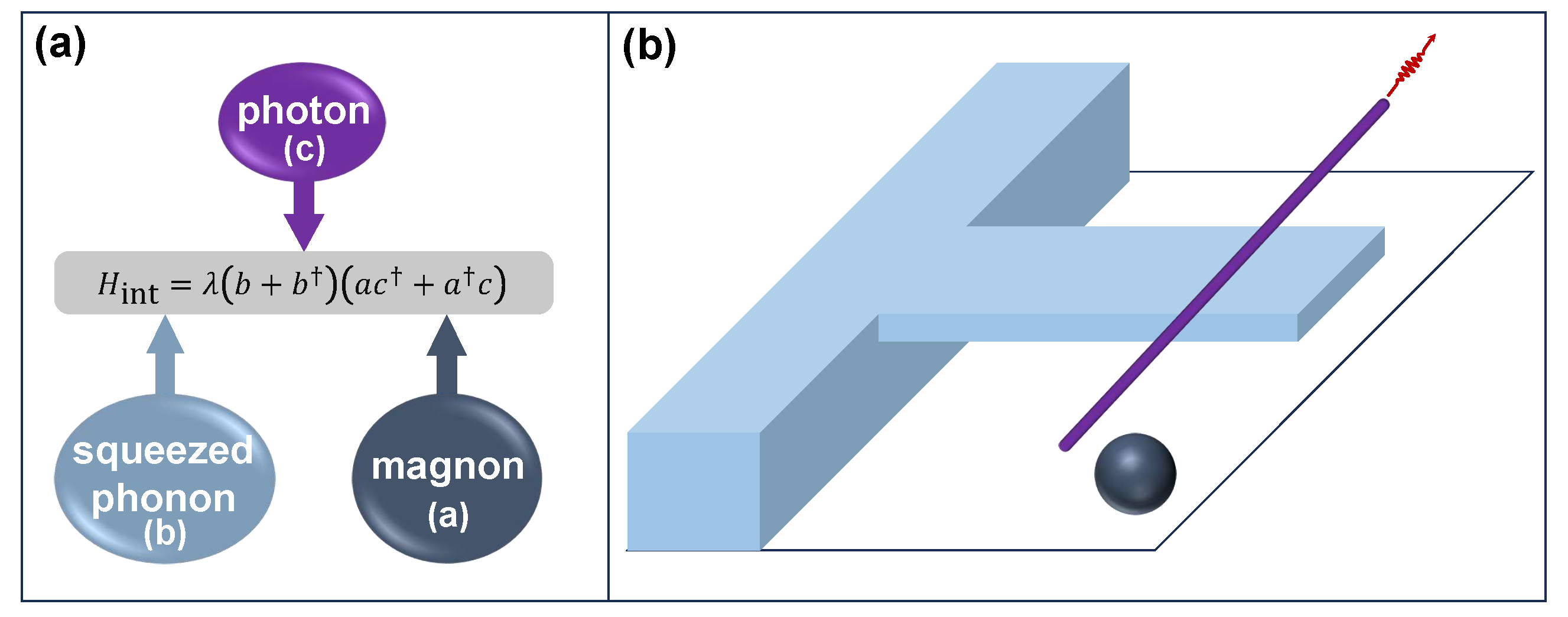
Motivated by this established mechanism, we adopt an analogous approach in a magnon-photon-phonon system to engineer the desired three-body interaction and thereby enable controllable dissipation channels. As illustrated in Figure 1, we consider a system comprising a magnon mode (a YIG microsphere), a photon mode (a transmission line), and a phonon mode (a cantilever). The interaction Hamiltonian is given by:

$$H_{\mathrm{int}}=\lambda (b+b^{†})(a{c}^{†}+a^{†}c),$$

(15)

where a, b, and c denote the annihilation operators for the magnon, phonon, and photon modes, respectively. When the cavity photon mode is strongly lossy, i.e., with a decay rate much larger than the coupling strengths, the nonlinear pump intensity or the Kerr coefficient of the magnon mode (${\Gamma }_{\mathrm{cav}}\gg \lambda ,s_a,K$), the pump field keeps in the steady state and adiabatically changes during the evolution. Therefore, this interaction Hamiltonian is capable of inducing a dissipation channel following the procedure of adiabatic elimination:

$$L=-(b+b^{†})a,$$

(16)

with a dissipation rate ${\Gamma }_{\mathrm{control}}={\lambda }^2/{\Gamma }_{\mathrm{cav}}$ (see also Appendix A). By manipulating the quantum state of the phonon mode, the effective loss rate in the magnon mode can be precisely tuned. Note that such loss is artificially induced loss, which is different from the intrinsic loss in Equation (9).

Reference [53] demonstrated that the coupling strength between the magnon, spin, and phonon modes can be enhanced by applying squeezing to the mechanical mode:

$$U\left(r\right)=exp\left({\displaystyle \frac{r(b^2-b^{†2})}{2}}\right),$$

(17)

where r is the squeezing parameter. This method further allows for the potential tuning of the loss rate of the dissipation channel induced by the three-body interaction in Equation (16). Given that the Lindblad operator in Equation (16) is proportional to the dimensionless position operator of the mechanical mode, $x\equiv (b+b^{†})/\sqrt{2}$, the squeezing or anti-squeezing of the position may modulate the decay rate.

It is noteworthy that the objective of this section is to modulate the overall system’s net dissipation rate using the squeezing effect. We will first introduce the theoretical model for mechanical mode squeezing incorporating loss and nonlinear pump. Subsequently, the control effects of mechanical-mode squeezing on magnon-mode dissipation will be elucidated. The detailed design for switchable collective loss will be presented in the subsequent section.

2.1. Effects of Mechanical-Mode Squeezing

To elucidate how phonon squeezing in the dissipation channel characterized by Equation (16) influences the loss of the magnon mode, we first introduce squeezing terms for the mechanical mode [53], which is at frequency ${\omega }_b$, following the same derivation mechanism as that employed for the magnon squeezing Hamiltonian in Equation (8).

$$H_{\mathrm{b}}=s_b^{*}{b}^{†}{b}^{†}+s_{b}bb,$$

(18)

where b is the phonon annihilation operator, and $s_b$ is the nonlinear pump intensity of the phonon mode, which governs the degree of squeezing in either the displacement or momentum quadrature. Such a nonlinear pump can be comparable to the loss, e.g., $\left|s_b\right|\approx 50\mathrm{kHz}$ for an oscillator with ${\gamma }_{\mathrm{m}}\approx 100\mathrm{kHz}$ [92], so that the control of mechanical squeezing is possible. It should be noted that we employ the displacement and momentum operators of the phonon mode here:

$$x={\displaystyle \frac{b+b^{†}}{\sqrt{2}}},p=i{\displaystyle \frac{b^{†}-b}{\sqrt{2}}}.$$

(19)

The squeezed quadrature is determined by the phase of $s_b$, namely, the phase of the pump field. A positive $s_b$ induces position squeezing ($\langle {(x-\langle x\rangle )}^2\rangle <{\displaystyle \frac{1}{2}}$), whereas a negative $s_b$ yields momentum squeezing ($\langle {(p-\langle p\rangle )}^2\rangle <{\displaystyle \frac{1}{2}}$) [93].

To maintain the mechanical mode in its steady state, we introduce a strong dissipation term described by the Lindblad operator:

$$L_b=b,$$

(20)

with a dissipation rate ${\Gamma }_b=10s_a$. Such a strong dissipation manifests a two-fold effect: Firstly, it suppresses the mechanical mode from entering the parametric instability regime. Secondly, this dissipation term suppresses the back-action of the magnon mode on the mechanical mode during the process of controlling the magnon mode via the mechanical mode.

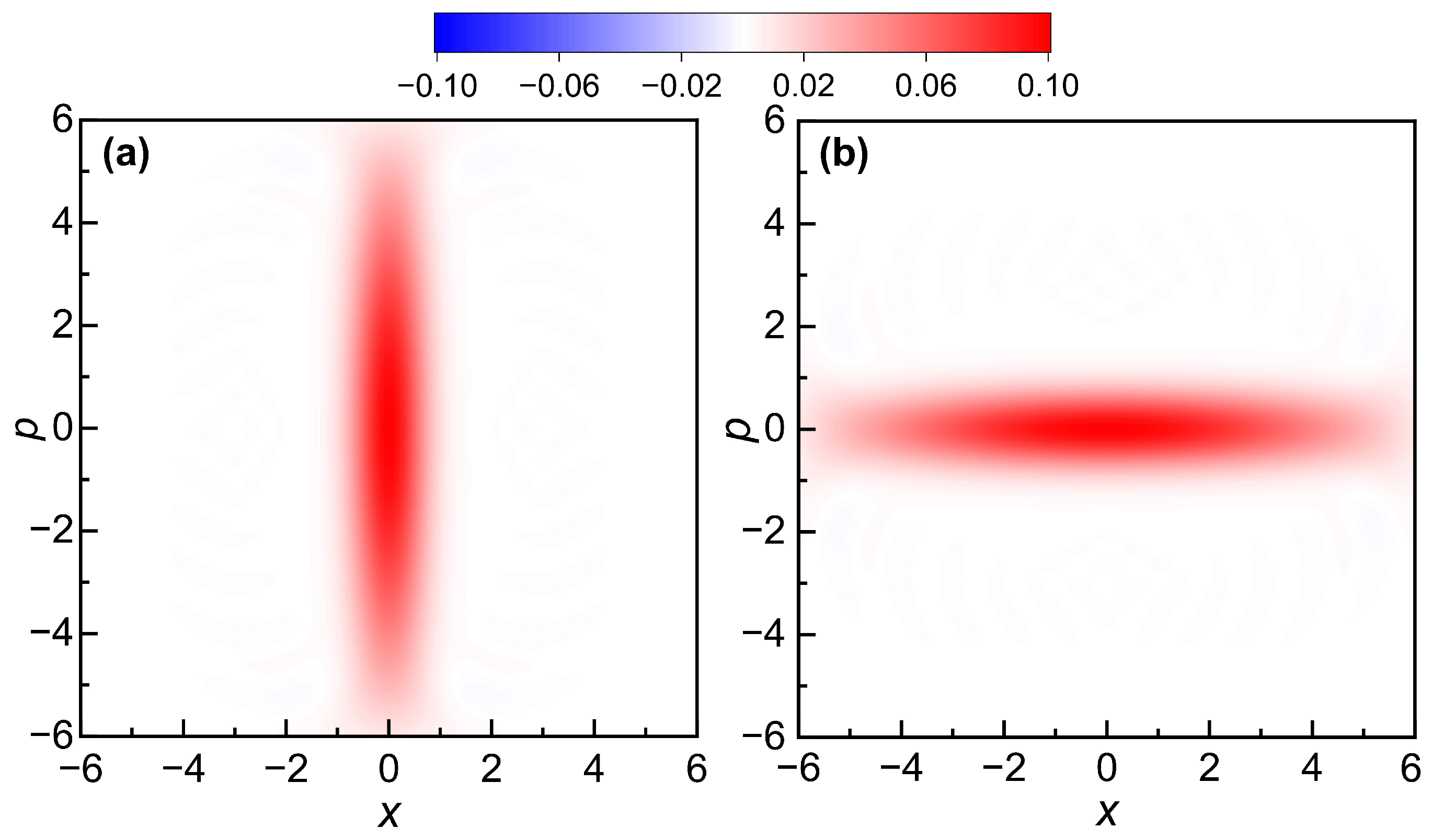
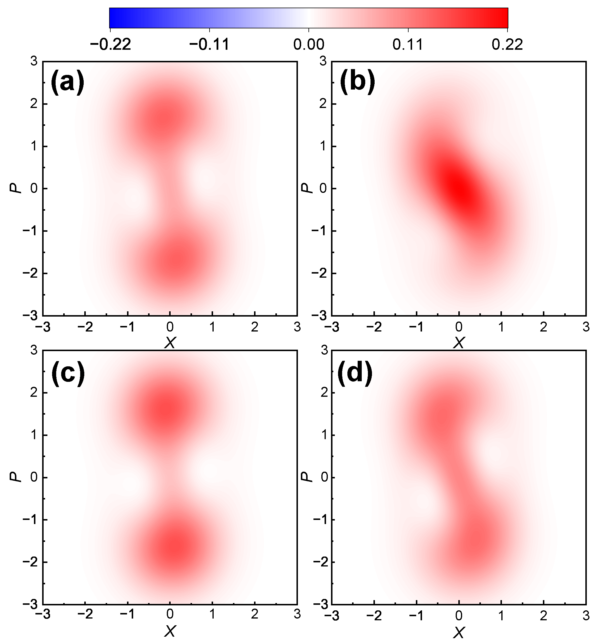
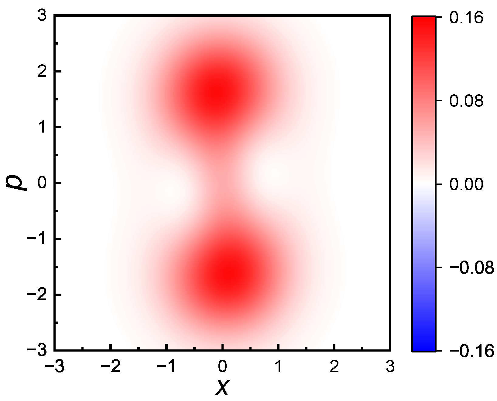
We perform numerical simulations of the mechanical system’s evolution using the Qutip package (v5.1.1), and the resultant Wigner function after a sufficiently long evolution time is illustrated in Figure 2. Corresponding to different pump phases, squeezing is observed in the position quadrature and the momentum quadrature, respectively. It is straightforward to anticipate that such squeezing can influence the dissipation described in Equation (16).

2.2. Switchable Loss in Single-Magnon System

This section investigates the influence of squeezing in the mechanical mode b on the magnon mode a and presents the foundational concept of switchable dissipation. The magnon mode under investigation is subject to a nonlinear pump (8), a nonlinear Kerr term (5), and controllable dissipation (16). Under the strong dissipation regime, the magnon steady state is characterized as a squeezed state, whereas bifurcation occurs in the weak dissipation limit [94]. In order to modulate the dissipation strength of the magnon mode, we introduce a two-phonon pump term (18) and a dissipation term (20) for the mechanical mode. As demonstrated in Figure 2, the squeezed quadrature can be selected via the pump phase, so that the loss term shown in Equation (16) can be adjusted.

The Hamiltonian of the system studied in the rotating frame is

$$H_{\mathrm{total}}=s_a^{*}{a}^{†}{a}^{†}+s_{a}aa+K{a}^{†}{a}^{†}aa+s_b^{*}{b}^{†}{b}^{†}+s_{b}bb,$$

(21)

where $s_a$ and K are, respectively, the nonlinear pump coefficient and the Kerr strength of the magnon mode. The nonlinear pump coefficient of the mechanical mode is described by $s_b$. The system’s overall dissipation is described by two loss channels:

$$\begin{array}{ccc}\hfill L_{\mathrm{control}}& =& -(b+b^{†})a,\hfill \\ \hfill L_b& =& b.\hfill \end{array}$$

(22)

Consistent with the preceding sections, we designate the loss rate of the mechanical mode as ${\Gamma }_b$ and that of the controllable channel as ${\Gamma }_{\mathrm{control}}$.

We prepare the initial state of the system in the vacuum state and perform numerical simulations of its dynamical evolution. Figure 3 illustrates the long-time-limit Wigner functions of the system under various parameter settings. The magnon squeezing coefficient is set to $s_a=1$, and is employed as the common unit for all other parameters. The truncation dimension of the Hilbert space is set to $N=20$. The remaining parameters are specified as ${\Gamma }_b=10$, ${\Gamma }_{\mathrm{control}}=0.64$, and $K=0.75$. In Figure 3a,b, we adopt a strong nonlinear pump $\left|s_b\right|=2.4$, a value close to the parametric stability threshold. In Figure 3a, the phonon squeezing coefficient is set to the position quadrature $s_b=2.4i$, and the Wigner function exhibits two separated components, unequivocally revealing the emergence of a bistable state. This bistable characteristic is indicative of weak dissipation in the magnon mode. In Figure 3b, the mechanical mode squeezing is switched to the momentum quadrature, with $s_b=-2.4i$. The corresponding Wigner function transforms into a single-component squeezed state, which indicates the presence of strong dissipation in the magnon mode. In Figure 3c,d, we consider a weaker squeezing intensity for the mechanical mode $\left|s_b\right|=1.5$, and demonstrate the performance of the switchable dissipation. In Figure 3c, the squeezing is in the position quadrature, consequently leading to a clear separation of the two components in the Wigner function. In Figure 3d, the squeezing is switched to the momentum quadrature; however, the Wigner function still exhibits two less-separated components. Therefore, even though the adjustable range is smaller, weak squeezing can still realize a tunable dissipation channel.

3. Switchable Collective Loss with Three-Body Coupling

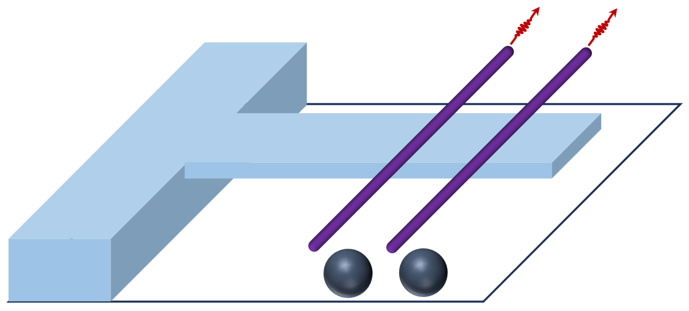
In Section 2, we introduced the fundamental concept of controlling the loss in a magnon mode via three-body coupling and squeezing. We now extend this idea to collective loss and achieve switchable dissipative coupling. As illustrated in Figure 4, the system under consideration comprises two YIG microspheres, two transmission lines, and a single cantilever. Two conducting wires introduce distinct forms of collective dissipation to these two magnon modes, which are defined in Equations (13) and (14). In addition, these two collective loss channels can be adjusted by the motion of the cantilever so that the dominant collective loss between the two magnon modes can be switched.

In this system, the squeezing of the mechanical mode plays a pivotal role in regulating the collective dissipation. The Hamiltonian and the dissipation of this part remain identical to those presented in Equations (18) and (20). Concurrently, nonlinear pump and Kerr terms are present in both YIG microspheres, which can be described by,

$$\begin{array}{c}\hfill \begin{array}{cc}\hfill H_{\mathrm{s}}=& H_{\mathrm{s},1}+H_{\mathrm{s},2}\hfill \\ \hfill =& s_a^{*}{a}_1^{†}{a}_1^{†}+s_a{a}_1{a}_1+s_a^{*}{a}_2^{†}{a}_2^{†}+s_a{a}_2{a}_2,\hfill \end{array}\end{array}$$

(23)

and,

$$\begin{array}{cc}\hfill H_{\mathrm{self}\text{-}\mathrm{kerr}}& =H_{\mathrm{self}\text{-}\mathrm{kerr},1}+H_{\mathrm{self}\text{-}\mathrm{kerr},2}\hfill \\ & =K{a}_1^{†}{a}_1^{†}{a}_1{a}_1+K{a}_2^{†}{a}_2^{†}{a}_2{a}_2.\hfill \end{array}$$

(24)

Such a system is commonly considered in studies for Kerr cat states [94,95,96], which has a steady state with the form of a two-mode separable cat state,

$$\begin{array}{c}\hfill |\psi \rangle ={\displaystyle \frac{1}{N_{\mathrm{tsc}}}}\left(\right|\alpha \rangle +|-\alpha \rangle )\left(\right|\alpha \rangle +|-\alpha \rangle ),\end{array}$$

(25)

with the normalization factor $N_{\mathrm{tsc}}$. With the presence of coupling, this steady state can be turned into states with different correlations, e.g., the even cat state $\left(\right|\alpha \rangle |\alpha \rangle +|-\alpha \rangle |-\alpha \rangle )/N_{\mathrm{ec}}$ or the odd cat state $\left(\right|\alpha \rangle |-\alpha \rangle +|-\alpha \rangle |\alpha \rangle )/N_{\mathrm{oc}}$.

Next, we introduce the switchable coupling part to modulate the steady states of the system. Two conducting wires can be modeled as two cavity modes with strong loss [97,98,99,100]:

$$\begin{array}{c}\hfill \begin{array}{cc}\hfill H_c=& {\omega }_c{c}_1^{†}{c}_1+{\omega }_c{c}_2^{†}{c}_2,\hfill \\ & L_1=c_1,L_2=c_2,\hfill \end{array}\end{array}$$

(26)

with cavity frequency ${\omega }_c$ and cavity mode loss rate ${\Gamma }_{\mathrm{cav}}$. Following the form of the tripartite coupling Hamiltonian used in Ref. [53], the three-body interactions among photon, phonon, and magnon modes are described by:

$$\begin{array}{c}{H}_{\mathrm{int},1}={\lambda }_{\mathrm{c}}(b+b^{†})[(a_1+a_2)c_1^{†}+{(a_1+a_2)}^{†}{c}_1],\hfill \\ H_{\mathrm{int},2}={\lambda }_{\mathrm{c}}i(b-b^{†})[(a_1-a_2)c_2^{†}+{(a_1-a_2)}^{†}{c}_2].\hfill \end{array}$$

(27)

Here, ${\lambda }_{\mathrm{c}}$ represents the coupling strength among the different components, which can reach the order of $\mathrm{MHz}$ [53]. These two cavity modes exhibit different coupling mechanisms to the magnon and mechanical modes, with the interactions defined by $H_{\mathrm{int},2}$ and $H_{\mathrm{int},1}$, respectively. Regarding the cavity-magnon coupling, one cavity mode couples in-phase to the two magnon modes, while the other cavity mode couples out-of-phase to the same two magnon modes. Such distinct collective couplings can induce the different collective dissipations presented in Equations (13) and (14). To enable switching between the different dissipation channels, the two cavity modes also exhibit distinct coupling forms to the mechanical mode. These differing coupling forms can be adjusted by varying the phases.

The cavity modes can be adiabatically eliminated if the loss rate in the cavities is much larger than the nonlinear coupling ${\Gamma }_{\mathrm{cav}}\gg {\lambda }_{\mathrm{c}}$. After the adiabatic elimination of the two cavity modes, the interaction terms in Equation (27) turn into two distinct loss channels described by the Lindblad operators (see also Appendix B):

$$\begin{array}{c}{L}_1=(b+b^{†})(a_1+a_2),\hfill \\ L_2=i(b^{†}-b)(a_1-a_2),\hfill \end{array}$$

(28)

with the loss rate ${\Gamma }_{\mathrm{cc}}={\lambda }_{\mathrm{c}}^2/{\Gamma }_{\mathrm{cav}}$. According to the previous estimation of ${\lambda }_{\mathrm{c}}$, this loss rate is about ${\Gamma }_{\mathrm{cc}}\approx 0.1\mathrm{MHz}$. Although the loss rate of these nonlinear Lindblad operators is given by the nonlinear coupling strength ${\lambda }_{\mathrm{c}}$ and the cavity mode loss, the dissipation in the magnon modes can still be influenced by the state of the mechanical mode. Given that these two dissipation channels are related to the position and momentum quadratures, respectively, we can utilize squeezing in different quadratures to control the active dissipation channel.

3.1. Numerical Verification of the Switchable Dissipative Coupling

In this section, we show that the nonlinear Lindblad operators in Equation (28) can realize the switching between two distinct dissipative couplings. The system under consideration is composed of three distinct parts: the magnon part, the collective dissipation part, and the mechanical part. The magnon part comprises two magnon modes, whose nonlinear pump and Kerr nonlinearity are described by Equations (23) and (24), respectively. The dissipative coupling is achieved via the dissipation channels presented in Equation (28). The mechanical mode is described by the Hamiltonian (18) and the local loss (20), which together can generate switchable squeezing. Note that a more rigorous check of the three-mode dissipative model is provided in Appendix C. As demonstrated in the previous section and other related works [35,94], without the dissipative coupling, these two magnon modes will evolve into a separable two-mode cat state. However, under the influence of the dissipative coupling, the system evolves into an entangled cat state. Moreover, the type of dissipative coupling dictates the relative phase between these two magnon modes, which can be verified using the joint Wigner function [101].

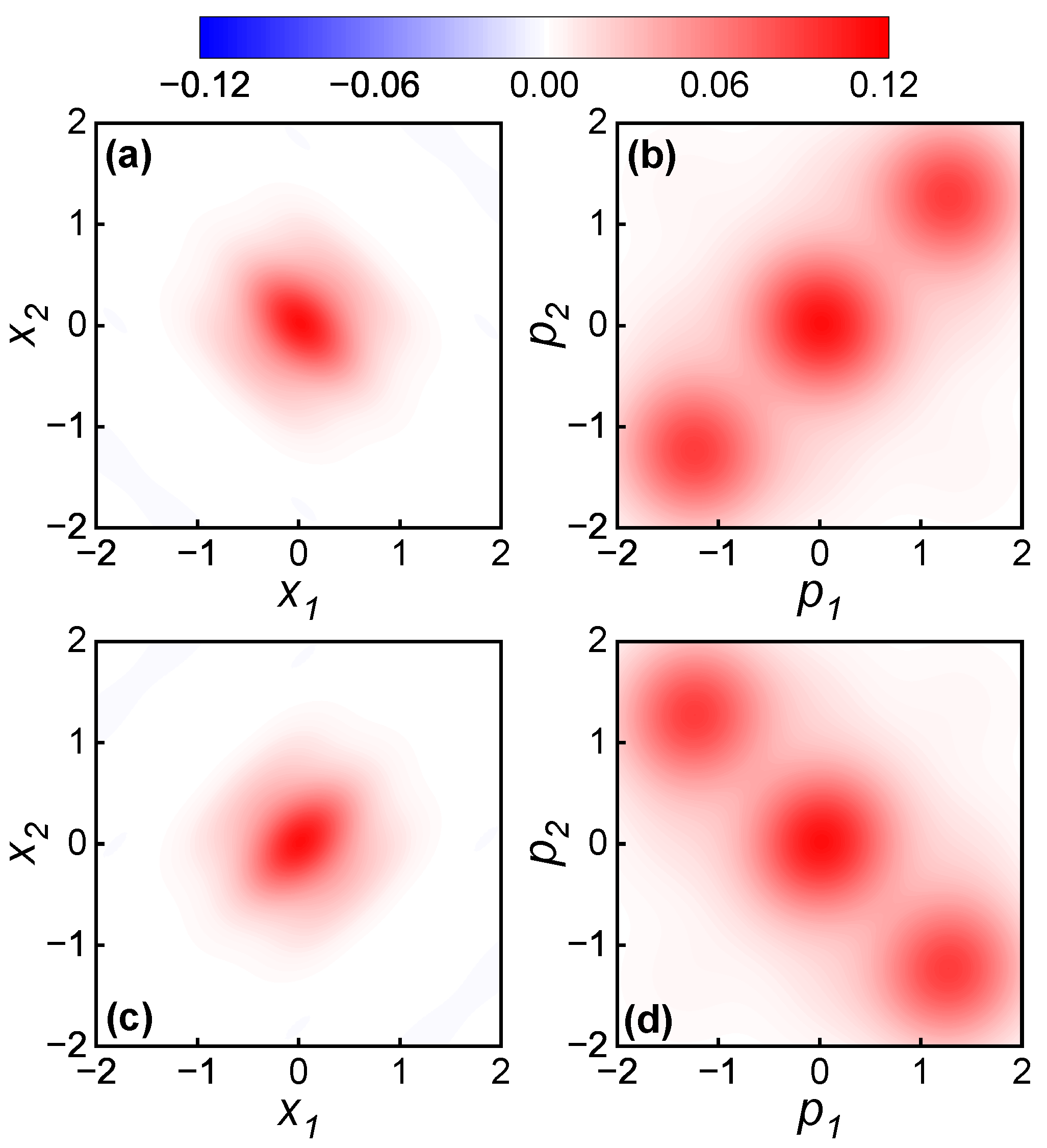
We set the initial state to the vacuum state and numerically simulate the system’s evolution using the Qutip package [102,103,104]. After a sufficiently long time evolution ($t=20s_a^{-1}$), we perform a partial trace over the mechanical mode and calculate the two-mode joint Wigner function [101] of the two remaining magnon modes. It should be noted that the joint Wigner function is a function in four-dimensional space; consequently, only two important cross-sections of this Wigner function are presented in Figure 5. Owing to the phase effect of the nonlinear pump in the magnon modes, the position cross-section of the joint Wigner function corresponds to the interference pattern, whereas the momentum cross-section corresponds to the two steady states of the magnon mode. In Figure 5a,b, we set the squeezing parameter of the mechanical mode to $s_b=2.4i$, so that the position quadrature is squeezed. Such position squeezing can suppress the loss channel $L_2$ in Equation (28) while enhancing $L_1$.

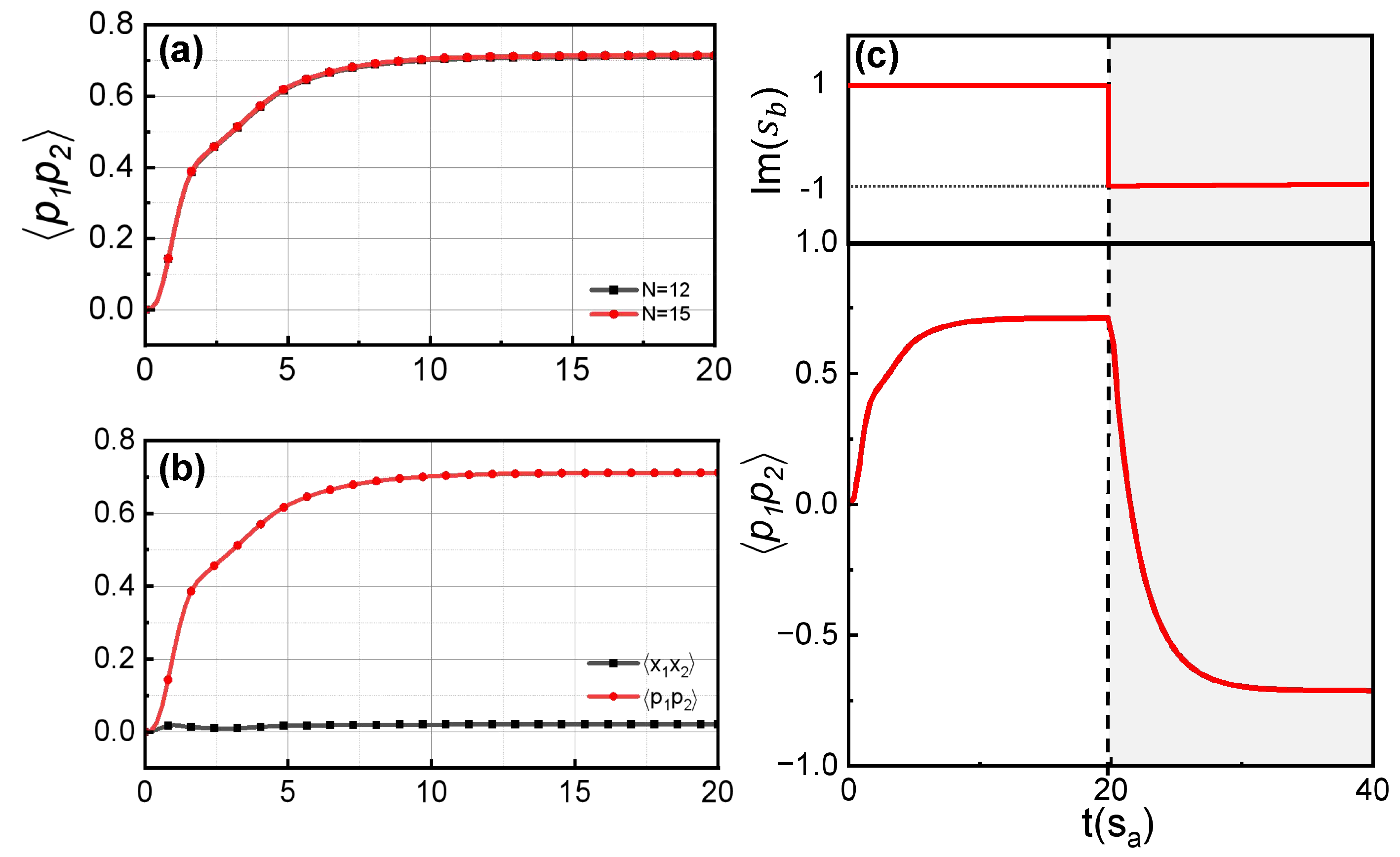
Although the joint Wigner function provides an intuitive visualization of the system, it is not suitable for characterizing its dynamical evolution. As a result, we use the correlation function of the magnon modes to illustrate the effect of the switchable dissipative coupling. Since the two components of the magnon mode reside in the momentum quadrature, as illustrated in Figure 3, we use the momentum correlation function to characterize the relative phase between the two magnon modes. The time evolution of the correlation function of the dimensionless momentum $\langle p_1{p}_2\rangle$ defined in Equation (19) is shown in Figure 6.

Figure 6a displays the time evolution of the momentum correlation function for different Hilbert space truncation dimensions. Specifically, the black curve corresponds to truncation $N=12$, and the red curve corresponds to $N=15$. The results obtained for $N=12$ are in complete agreement with those for $N=15$, indicating that a truncation dimension of $N=12$ is sufficient. In addition, under the influence of a ferromagnetic dissipative coupling $\mathrm{Im}\left(s_b\right)>0$, the time evolution of the correlation function is clearly observed to transition from its initial value of 0 to a steady-state value of approximately $0.7$. Figure 6b presents a comparison between the position correlation function (black curve) and the momentum correlation function (red curve). The position correlation function is negligible compared to the momentum correlation function, which validates our previous picture of effective spins being encoded in the momentum quadrature.

To illustrate the dynamical switching of the dissipative coupling, we consider a time-dependent nonlinear pump applied to the mechanical mode. This pump is initially set to $\mathrm{Im}\left(s_b\right)>0$ and is subsequently switched to $\mathrm{Im}\left(s_b\right)<0$, as depicted in the upper part of Figure 6c. The lower part of Figure 6c displays the time evolution of the momentum correlation function. The evolution prior to the switching of $s_b$ is consistent with the results presented in Figure 6a,b, i.e., the correlation function gradually approaches a steady positive value. Following the sign reversal of $s_b$, the correlation function begins to evolve toward a negative value, which corresponds to an antiferromagnetic alignment of the two optical spins. Therefore, our proposal enables the dynamical switching between different types of dissipative coupling.

3.2. Robustness of the Switchable Loss Channels

In the preceding section, we demonstrated the effects of switchable collective loss using the two-mode joint Wigner function and the momentum correlation function. We now consider the robustness of our proposal against other unwanted dissipation mechanisms. Note that the three-body coupling [53] is the first-order perturbation of the magnon-cavity coupling with respect to the mechanical mode. As a result, the zeroth order terms, which remain unmodified by the mechanical mode, can also contribute to the magnon loss. To investigate the influence of these zeroth-order contributions, we incorporate the following two loss channels,

$$\begin{array}{c}{L}_3=a_1+a_2,\hfill \\ L_4=a_1-a_2,\hfill \end{array}$$

(29)

with a significantly stronger loss rate ${\Gamma }_{\mathrm{ncc}}=4s_a$ compared to the switchable part ${\Gamma }_{\mathrm{cc}}=0.64s_a$. The uncontrollable loss rate ${\Gamma }_{\mathrm{ncc}}$ is usually less than $10\%$ of the magnon cavity coupling. For a typical coupling of $100\mathrm{MHz}$ [31], we can have ${\Gamma }_{\mathrm{ncc}}\approx 10\mathrm{MHz}$. To compensate for the additional loss, we introduce enhanced pumps into the magnon modes:

$${\tilde{H}}_{\mathrm{s}}={\tilde{s}}_a^{*}{a}_1^{†}{a}_1^{†}+{\tilde{s}}_a{a}_1{a}_1+{\tilde{s}}_a^{*}{a}_2^{†}{a}_2^{†}+{\tilde{s}}_a{a}_2{a}_2,$$

(30)

with ${\tilde{s}}_a=4.2s_a$. All other parameters remain consistent with those used in Figure 5 and Figure 6.

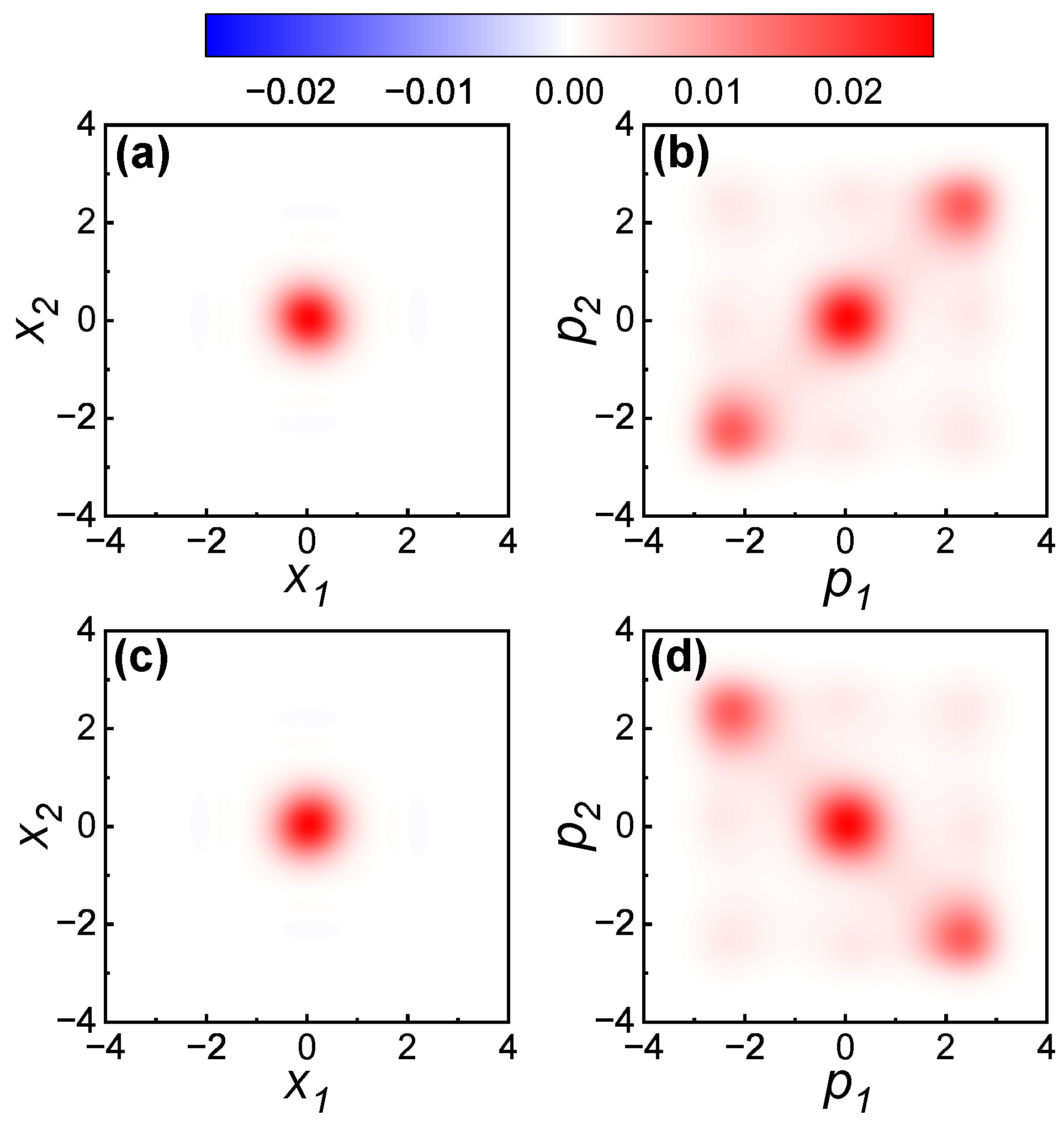
We first provide an intuitive picture by utilizing the joint Wigner function of the reduced magnon state, as illustrated in Figure 7. Figure 7 shows typical joint Wigner functions of catlike two-mode states, which can represent two correlated effective spins. In Figure 7a,b, the position quadrature of the mechanical mode is squeezed, consequently, the coupling assumes a ferromagnetic form. The two nonzero components in Figure 7b exhibit positive momentum correlations, which agree with the expected effects of a ferromagnetic dissipative coupling. In Figure 7c,d, the coupling is set to the antiferromagnetic form, and the two nonzero components in Figure 7d exhibit negative momentum correlations. These results demonstrate that the switchable dissipative coupling is still effective even under the influence of strong dissipation mechanisms that cannot be modified by the mechanical mode.

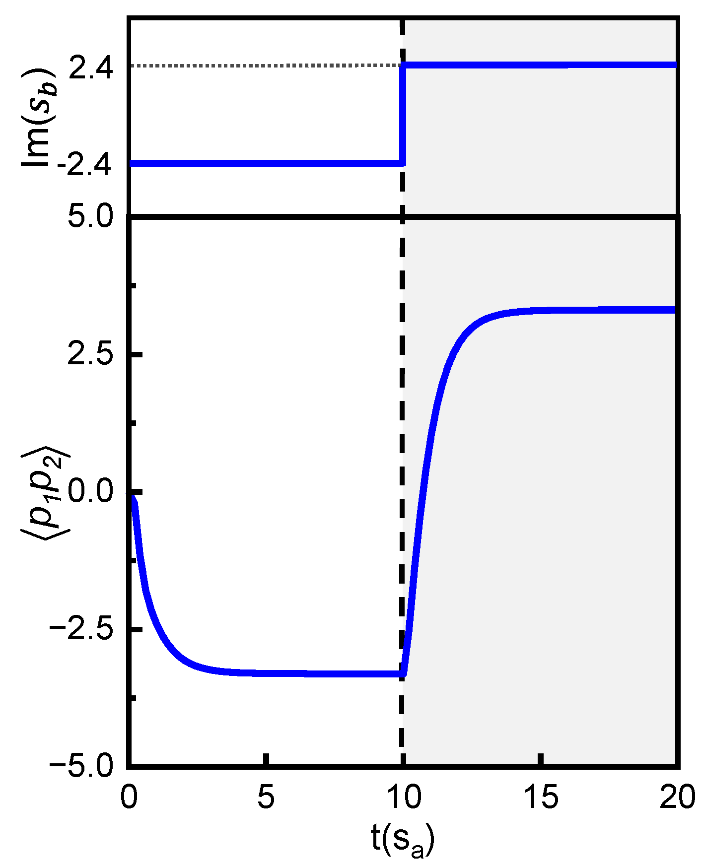
Following the approach of the preceding section, we employ the momentum correlation function to demonstrate the dynamical switching of the coupling. In Figure 8, the imaginary part of $s_b$ is first set to a negative value and is subsequently switched to a positive value after a period of time ($10s_a^{-1}$). The evolution of the momentum correlation function is consistent with the switching of the coupling. Therefore, the dynamical switching can also be achieved even under the influence of strong constant dissipation.

4. Results

We proposed a scheme to realize switchable dissipative coupling in magnon systems, based on three-body coupling, which is crucial for applying these systems in solving combinatorial optimization problems. The switchable dissipative coupling consists of two distinct collective dissipation channels induced by two open conducting wires, where the coupling to the magnon modes is modulated by a mechanical mode (i.e., three-body coupling). By modulating the phase of the nonlinear pump in the mechanical mode, the squeezed quadrature can be tuned to control the active dissipation channel. We numerically verified the effects of our proposal using two magnon modes coupled by the switchable dissipative coupling. The numerical results demonstrate that different control parameters in the mechanical mode lead to distinct relative phases between the two magnon modes, consistent with the design of the switchable coupling. Furthermore, switching during the dynamical evolution is also feasible. In addition, we investigated the influence of unwanted dissipation arising from the constant term of the magnon-wire coupling, which can be effectively compensated by incorporating stronger dissipation in the magnon modes.

Our work provides a potential pathway for the application of magnon systems in Ising machines for solving complex combinatorial optimization problems. These switchable couplings may also improve the performance of magnon systems in quantum computing and quantum communications.

References

1. Fransson, J.; Black-Schaffer, A.M.; Balatsky, A.V. Magnon Dirac materials. Phys. Rev. B 2016, 94, 075401. [Google Scholar] [CrossRef]
2. Chumak, A.V.; Serga, A.A.; Hillebrands, B. Magnon transistor for all-magnon data processing. Nat. Commun. 2014, 5, 4700. [Google Scholar] [CrossRef] [PubMed]
3. Rezende, S.M.; Azevedo, A.; Rodríguez-Suárez, R.L. Introduction to antiferromagnetic magnons. J. Appl. Phys. 2019, 126, 151101. [Google Scholar] [CrossRef]
4. Zhitomirsky, M.E.; Chernyshev, A.L. Colloquium: Spontaneous magnon decays. Rev. Mod. Phys. 2013, 85, 219–242. [Google Scholar] [CrossRef]
5. An, K.; Xu, M.; Mucchietto, A.; Kim, C.; Moon, K.W.; Hwang, C.; Grundler, D. Emergent coherent modes in nonlinear magnonic waveguides detected at ultrahigh frequency resolution. Nat. Commun. 2024, 15, 7302. [Google Scholar] [CrossRef] [PubMed]
6. Hula, T.; Schultheiss, K.; Buzdakov, A.; Körber, L.; Bejarano, M.; Flacke, L.; Liensberger, L.; Weiler, M.; Shaw, J.M.; Nembach, H.T.; et al. Nonlinear losses in magnon transport due to four-magnon scattering. Appl. Phys. Lett. 2020, 117, 042404. [Google Scholar] [CrossRef]
7. Zhang, G.Q.; Wang, Y.; Xiong, W. Detection sensitivity enhancement of magnon Kerr nonlinearity in cavity magnonics induced by coherent perfect absorption. Phys. Rev. B 2023, 107, 064417. [Google Scholar] [CrossRef]
8. Schultheiss, H.; Vogt, K.; Hillebrands, B. Direct observation of nonlinear four-magnon scattering in spin-wave microconduits. Phys. Rev. B 2012, 86, 054414. [Google Scholar] [CrossRef]
9. Landeros, P.; Arias, R.E.; Mills, D.L. Two magnon scattering in ultrathin ferromagnets: The case where the magnetization is out of plane. Phys. Rev. B 2008, 77, 214405. [Google Scholar] [CrossRef]
10. Heinrich, B.; Cochran, J.F.; Hasegawa, R. FMR linebroadening in metals due to two-magnon scattering. J. Appl. Phys. 1985, 57, 3690–3692. [Google Scholar] [CrossRef]
11. Chumak, A.V.; Vasyuchka, V.I.; Serga, A.A.; Hillebrands, B. Magnon spintronics. Nat. Phys. 2015, 11, 453–461. [Google Scholar] [CrossRef]
12. Yuan, H.Y.; Cao, Y.; Kamra, A.; Duine, R.A.; Yan, P. Quantum magnonics: When magnon spintronics meets quantum information science. Phys. Rep. 2022, 965, 1–74. [Google Scholar] [CrossRef]
13. Brächer, T.; Pirro, P.; Hillebrands, B. Parallel pumping for magnon spintronics: Amplification and manipulation of magnon spin currents on the micron-scale. Phys. Rep. 2017, 699, 1–34. [Google Scholar] [CrossRef]
14. Tabuchi, Y.; Ishino, S.; Ishikawa, T.; Yamazaki, R.; Usami, K.; Nakamura, Y. Hybridizing Ferromagnetic Magnons and Microwave Photons in the Quantum Limit. Phys. Rev. Lett. 2014, 113, 083603. [Google Scholar] [CrossRef] [PubMed]
15. Woolsey, R.B.; White, R.M. Electron-Magnon Interaction in Ferromagnetic Semiconductors. Phys. Rev. B 1970, 1, 4474–4486. [Google Scholar] [CrossRef]
16. Chen, J.; Fan, X.G.; Xiong, W.; Wang, D.; Ye, L. Nonreciprocal entanglement in cavity-magnon optomechanics. Phys. Rev. B 2023, 108, 024105. [Google Scholar] [CrossRef]
17. Lachance-Quirion, D.; Tabuchi, Y.; Gloppe, A.; Usami, K.; Nakamura, Y. Hybrid quantum systems based on magnonics. Appl. Phys. Express 2019, 12, 070101. [Google Scholar] [CrossRef]
18. Khan, Q.; Abukhadra, M.R.; El-Sherbeeny, A.M.; Choi, J.R.; Ali, A.; Khan, M. Coherent manipulation of the surface plasmon resonance sensing at the dielectric-graphene interface under Cross-Kerr nonlinearity effect. J. Magn. Magn. Mater. 2025, 618, 172858. [Google Scholar] [CrossRef]
19. Zhang, Z.; Gneiting, C.; Zhou, Z.Y.; Chen, A.X. Cat-state-like non-Gaussian entanglement in magnon systems. Phys. Rev. A 2025, 111, 033717. [Google Scholar] [CrossRef]
20. Liu, D.W.; Wu, Y.; Si, L.G. Magnon cat states induced by photon parametric coupling. Phys. Rev. Appl. 2024, 21, 044018. [Google Scholar] [CrossRef]
21. Sun, F.X.; Zheng, S.S.; Xiao, Y.; Gong, Q.; He, Q.; Xia, K. Remote Generation of Magnon Schrödinger Cat State via Magnon-Photon Entanglement. Phys. Rev. Lett. 2021, 127, 087203. [Google Scholar] [CrossRef] [PubMed]
22. Kong, C.; Xiong, H.; Wu, Y. Magnon-Induced Nonreciprocity Based on the Magnon Kerr Effect. Phys. Rev. Appl. 2019, 12, 034001. [Google Scholar] [CrossRef]
23. Haghshenasfard, Z.; Cottam, M.G. Sub-Poissonian statistics and squeezing of magnons due to the Kerr effect in a hybrid coupled cavity–magnon system. J. Appl. Phys. 2020, 128, 033901. [Google Scholar] [CrossRef]
24. Kamra, A.; Belzig, W.; Brataas, A. Magnon-squeezing as a niche of quantum magnonics. Appl. Phys. Lett. 2020, 117, 090501. [Google Scholar] [CrossRef]
25. Ji, F.Z.; An, J.H. Kerr nonlinearity induced strong spin-magnon coupling. Phys. Rev. B 2023, 108, L180409. [Google Scholar] [CrossRef]
26. Tomita, S.; Kato, T.; Tsunashima, S.; Iwata, S.; Fujii, M.; Hayashi, S. Magneto-Optical Kerr Effects of Yttrium-Iron Garnet Thin Films Incorporating Gold Nanoparticles. Phys. Rev. Lett. 2006, 96, 167402. [Google Scholar] [CrossRef] [PubMed]
27. Wang, Y.P.; Zhang, G.Q.; Zhang, D.; Luo, X.Q.; Xiong, W.; Wang, S.P.; Li, T.F.; Hu, C.M.; You, J.Q. Magnon Kerr effect in a strongly coupled cavity-magnon system. Phys. Rev. B 2016, 94, 224410. [Google Scholar] [CrossRef]
28. Zhou, Y.; Xie, S.Y.; Zhu, C.J.; Yang, Y.P. Nonlinear pumping induced multipartite entanglement in a hybrid magnon cavity QED system. Phys. Rev. B 2022, 106, 224404. [Google Scholar] [CrossRef]
29. Goryachev, M.; Farr, W.G.; Creedon, D.L.; Fan, Y.; Kostylev, M.; Tobar, M.E. High-Cooperativity Cavity QED with Magnons at Microwave Frequencies. Phys. Rev. Appl. 2014, 2, 054002. [Google Scholar] [CrossRef]
30. Makiuchi, T.; Hioki, T.; Shimazu, Y.; Oikawa, Y.; Yokoi, N.; Daimon, S.; Saitoh, E. Parametron on magnetic dot: Stable and stochastic operation. Appl. Phys. Lett. 2021, 118, 022402. [Google Scholar] [CrossRef]
31. Wang, Y.P.; Zhang, G.Q.; Zhang, D.; Li, T.F.; Hu, C.M.; You, J.Q. Bistability of Cavity Magnon Polaritons. Phys. Rev. Lett. 2018, 120, 057202. [Google Scholar] [CrossRef] [PubMed]
32. Pan, H.; Yang, Y.; An, Z.H.; Hu, C.M. Bistability in dissipatively coupled cavity magnonics. Phys. Rev. B 2022, 106, 054425. [Google Scholar] [CrossRef]
33. Yang, Z.B.; Jin, H.; Jin, J.W.; Liu, J.Y.; Liu, H.Y.; Yang, R.C. Bistability of squeezing and entanglement in cavity magnonics. Phys. Rev. Res. 2021, 3, 023126. [Google Scholar] [CrossRef]
34. Zhang, G.Q.; Chen, Z.; Xiong, W.; Lam, C.H.; You, J.Q. Parity-symmetry-breaking quantum phase transition via parametric drive in a cavity magnonic system. Phys. Rev. B 2021, 104, 064423. [Google Scholar] [CrossRef]
35. Elyasi, M.; Saitoh, E.; Bauer, G.E.W. Stochasticity of the magnon parametron. Phys. Rev. B 2022, 105, 054403. [Google Scholar] [CrossRef]
36. Xie, S.; Raman, S.R.S.; Ni, C.; Wang, M.; Yang, M.; Kulkarni, J.P. Ising-CIM: A Reconfigurable and Scalable Compute Within Memory Analog Ising Accelerator for Solving Combinatorial Optimization Problems. IEEE J. Solid-State Circuits 2022, 57, 3453–3465. [Google Scholar] [CrossRef]
37. Wang, Z.; Marandi, A.; Wen, K.; Byer, R.L.; Yamamoto, Y. Coherent Ising machine based on degenerate optical parametric oscillators. Phys. Rev. A 2013, 88, 063853. [Google Scholar] [CrossRef]
38. Inagaki, T.; Haribara, Y.; Igarashi, K.; Sonobe, T.; Tamate, S.; Honjo, T.; Marandi, A.; McMahon, P.L.; Umeki, T.; Enbutsu, K.; et al. A coherent Ising machine for 2000-node optimization problems. Science 2016, 354, 603–606. [Google Scholar] [CrossRef] [PubMed]
39. Zha, J.; Su, J.; Li, T.; Cao, C.; Ma, Y.; Wei, H.; Huang, Z.; Qian, L.; Wen, K.; Zhang, J. Encoding Molecular Docking for Quantum Computers. J. Chem. Theory Comput. 2023, 19, 9018. [Google Scholar] [CrossRef] [PubMed]
40. Wen, J.; Wang, Z.; Huang, Z.; Cai, D.; Jia, B.; Cao, C.; Ma, Y.; Wei, H.; Wen, K.; Qian, L. Optical experimental solution for the multiway number partitioning problem and its application to computing power scheduling. Sci. China Phys. Mech. Astron. 2023, 66, 290313. [Google Scholar] [CrossRef]
41. Yamamoto, Y.; Leleu, T.; Ganguli, S.; Mabuchi, H. Coherent Ising machines—Quantum optics and neural network Perspectives. Appl. Phys. Lett. 2020, 117, 160501. [Google Scholar] [CrossRef]
42. Lu, B.; Fan, C.R.; Liu, L.; Wen, K.; Wang, C. Speed-up coherent Ising machine with a spiking neural network. Opt. Express 2023, 31, 3676–3684. [Google Scholar] [CrossRef] [PubMed]
43. Honjo, T.; Sonobe, T.; Inaba, K.; Inagaki, T.; Ikuta, T.; Yamada, Y.; Kazama, T.; Enbutsu, K.; Umeki, T.; Kasahara, R.; et al. 100,000-spin coherent Ising machine. Sci. Adv. 2021, 7, eabh0952. [Google Scholar] [CrossRef] [PubMed]
44. Aonishi, T.; Nagasawa, T.; Koizumi, T.; Gunathilaka, M.D.S.H.; Mimura, K.; Okada, M.; Kako, S.; Yamamoto, Y. Highly Versatile FPGA-Implemented Cyber Coherent Ising Machine. IEEE Access 2024, 12, 175843–175865. [Google Scholar] [CrossRef]
45. Mohseni, N.; McMahon, P.L.; Byrnes, T. Ising machines as hardware solvers of combinatorial optimization problems. Nat. Rev. Phys. 2022, 4, 363–379. [Google Scholar] [CrossRef]
46. Hamerly, R.; Inagaki, T.; McMahon, P.L.; Venturelli, D.; Marandi, A.; Onodera, T.; Ng, E.; Langrock, C.; Inaba, K.; Honjo, T.; et al. Experimental investigation of performance differences between coherent Ising machines and a quantum annealer. Sci. Adv. 2019, 5, eaau0823. [Google Scholar] [CrossRef] [PubMed]
47. Ng, E.; Onodera, T.; Kako, S.; McMahon, P.L.; Mabuchi, H.; Yamamoto, Y. Efficient sampling of ground and low-energy Ising spin configurations with a coherent Ising machine. Phys. Rev. Res. 2022, 4, 013009. [Google Scholar] [CrossRef]
48. Takesue, H.; Yamada, Y.; Inaba, K.; Ikuta, T.; Yonezu, Y.; Inagaki, T.; Honjo, T.; Kazama, T.; Enbutsu, K.; Umeki, T.; et al. Observing a Phase Transition in a Coherent Ising Machine. Phys. Rev. Appl. 2023, 19, L031001. [Google Scholar] [CrossRef]
49. Calvanese Strinati, M.; Pierangeli, D.; Conti, C. All-Optical Scalable Spatial Coherent Ising Machine. Phys. Rev. Appl. 2021, 16, 054022. [Google Scholar] [CrossRef]
50. Ezawa, M.; Lebrasseur, E.; Mita, Y. Ising Machine Based on Bistable Microelectromechanical Systems. J. Phys. Soc. Jpn. 2022, 91, 114601. [Google Scholar] [CrossRef]
51. Marandi, A.; Wang, Z.; Takata, K.; Byer, R.L.; Yamamoto, Y. Network of time-multiplexed optical parametric oscillators as a coherent Ising machine. Nat. Photonics 2014, 8, 937–942. [Google Scholar] [CrossRef]
52. McMahon, P.L.; Marandi, A.; Haribara, Y.; Hamerly, R.; Langrock, C.; Tamate, S.; Inagaki, T.; Takesue, H.; Utsunomiya, S.; Aihara, K.; et al. A fully programmable 100-spin coherent Ising machine with all-to-all connections. Science 2016, 354, 614–617. [Google Scholar] [CrossRef] [PubMed]
53. Hei, X.L.; Li, P.B.; Pan, X.F.; Nori, F. Enhanced Tripartite Interactions in Spin-Magnon-Mechanical Hybrid Systems. Phys. Rev. Lett. 2023, 130, 073602. [Google Scholar] [CrossRef] [PubMed]
54. Chen, X.C.; Wang, Z.J.; Zheng, S.B.; Chen, J.; Xiong, W. Exponentially enhanced tripartite coupling in quantum nonlinear magnonics. Phys. Rev. A 2025, 112, 063730. [Google Scholar] [CrossRef]
55. Shen, Z.; Xu, G.T.; Zhang, M.; Zhang, Y.L.; Wang, Y.; Chai, C.Z.; Zou, C.L.; Guo, G.C.; Dong, C.H. Coherent Coupling between Phonons, Magnons, and Photons. Phys. Rev. Lett. 2022, 129, 243601. [Google Scholar] [CrossRef] [PubMed]
56. Amazioug, M.; Teklu, B.; Asjad, M. Enhancement of magnon–photon–phonon entanglement in a cavity magnomechanics with coherent feedback loop. Sci. Rep. 2023, 13, 3833. [Google Scholar] [CrossRef] [PubMed]
57. Li, J.; Zhu, S.Y.; Agarwal, G.S. Magnon-Photon-Phonon Entanglement in Cavity Magnomechanics. Phys. Rev. Lett. 2018, 121, 203601. [Google Scholar] [CrossRef] [PubMed]
58. Qi, S.F.; Jing, J. Magnon-assisted photon-phonon conversion in the presence of structured environments. Phys. Rev. A 2021, 103, 043704. [Google Scholar] [CrossRef]
59. Chen, Q.G.; Liu, M.Y.; Huang, X.X.; Chen, J.; Xiong, W. Hybrid cavity-magnon optomechanics: Tailoring bipartite and tripartite macroscopic entanglement. Chaos Solitons Fractals 2026, 202, 117472. [Google Scholar] [CrossRef]
60. Imai, S.; Tsuji, N. Quantum many-body scars with unconventional superconducting pairing symmetries via multibody interactions. Phys. Rev. Res. 2025, 7, 013064. [Google Scholar] [CrossRef]
61. Xiong, W.; Tian, M.; Zhang, G.Q.; You, J.Q. Strong long-range spin-spin coupling via a Kerr magnon interface. Phys. Rev. B 2022, 105, 245310. [Google Scholar] [CrossRef]
62. Chen, J.; Xiong, W.; Wang, D.; Ye, L. Strong and noise-tolerant entanglement in dissipative optomechanics. Phys. Rev. A 2025, 111, 053512. [Google Scholar] [CrossRef]
63. Wang, Y.; Xiong, W.; Xu, Z.; Zhang, G.Q.; You, J.Q. Dissipation-induced nonreciprocal magnon blockade in a magnon-based hybrid system. Sci. China Phys. Mech. Astron. 2022, 65, 260314. [Google Scholar] [CrossRef]
64. Liang, Z.; Li, J.; Wu, Y. All-optical polarization-state engineering in quantum cavity optomagnonics. Phys. Rev. A 2023, 107, 033701. [Google Scholar] [CrossRef]
65. Chen, Y.; Wang, Y.; You, J.; Liu, Y.; Yi, S.; Deng, Y. Atom-molecule superradiance and entanglement with cavity-mediated three-body interactions. Phys. Rev. Appl. 2026, 25, 024019. [Google Scholar] [CrossRef]
66. Zhao, G.; Wang, Y.; Qian, X.F. Driven dissipative quantum dynamics in a cavity magnon-polariton system. Phys. Rev. B 2021, 104, 134423. [Google Scholar] [CrossRef]
67. Xiao, Y.; Xia, K. Dissipation-induced magnon-photon entanglement in a squeezed vacuum reservoir. Phys. Rev. B 2025, 111, 064414. [Google Scholar] [CrossRef]
68. Liu, G.; Xiong, W.; Ying, Z.J. Switchable superradiant phase transition with Kerr magnons. Phys. Rev. A 2023, 108, 033704. [Google Scholar] [CrossRef]
69. Annby-Andersson, B.; Bakhshinezhad, F.; Bhattacharyya, D.; De Sousa, G.; Jarzynski, C.; Samuelsson, P.; Potts, P.P. Quantum Fokker-Planck Master Equation for Continuous Feedback Control. Phys. Rev. Lett. 2022, 129, 050401. [Google Scholar] [CrossRef] [PubMed]
70. Amazioug, M.; Singh, S.; Teklu, B.; Asjad, M. Feedback control of quantum correlations in a cavity magnomechanical system with magnon squeezing. Entropy 2023, 25, 1462. [Google Scholar] [CrossRef]
71. Zhang, G.Q.; Feng, W.; Xiong, W.; Su, Q.P.; Yang, C.P. Generation of long-lived W states via reservoir engineering in dissipatively coupled systems. Phys. Rev. A 2023, 107, 012410. [Google Scholar] [CrossRef]
72. Zanardi, P.; Campos Venuti, L. Coherent Quantum Dynamics in Steady-State Manifolds of Strongly Dissipative Systems. Phys. Rev. Lett. 2014, 113, 240406. [Google Scholar] [CrossRef] [PubMed]
73. Valenti, D.; Carollo, A.; Spagnolo, B. Stabilizing effect of driving and dissipation on quantum metastable states. Phys. Rev. A 2018, 97, 042109. [Google Scholar] [CrossRef]
74. Ao, P.; Rammer, J. Quantum dynamics of a two-state system in a dissipative environment. Phys. Rev. B 1991, 43, 5397–5418. [Google Scholar] [CrossRef] [PubMed]
75. Blundell, S. Magnetism in Condensed Matter; Oxford University Press: Oxford, UK, 2001. [Google Scholar] [CrossRef]
76. Macdonald, J. Ferromagnetic resonance and the internal field in ferromagnetic materials. Proc. Phys. Soc. A 1951, 64, 968–983. [Google Scholar] [CrossRef]
77. Soykal, O.O.; Flatté, M.E. Strong Field Interactions between a Nanomagnet and a Photonic Cavity. Phys. Rev. Lett. 2010, 104, 077202. [Google Scholar] [CrossRef] [PubMed]
78. Holstein, T.; Primakoff, H. Field Dependence of the Intrinsic Domain Magnetization of a Ferromagnet. Phys. Rev. 1940, 58, 1098–1113. [Google Scholar] [CrossRef]
79. Sheng, L.; Elyasi, M.; Chen, J.; He, W.; Wang, Y.; Wang, H.; Feng, H.; Zhang, Y.; Medlej, I.; Liu, S.; et al. Nonlocal Detection of Interlayer Three-Magnon Coupling. Phys. Rev. Lett. 2023, 130, 046701. [Google Scholar] [CrossRef] [PubMed]
80. Wang, Y.; Wu, J.L.; Jiao, Y.F.; Lu, T.X.; Zhang, H.L.; Jiang, L.Y.; Kuang, L.M.; Jing, H. Enhancing tripartite photon-phonon-magnon entanglement by synergizing parametric amplifications. Phys. Rev. A 2025, 111, 013709. [Google Scholar] [CrossRef]
81. Yuan, H.Y.; Sterk, W.P.; Kamra, A.; Duine, R.A. Master equation approach to magnon relaxation and dephasing. Phys. Rev. B 2022, 106, 224422. [Google Scholar] [CrossRef]
82. Weng, Y.C.; Xu, D.; Chen, Z.; Tan, L.Z.; Gu, X.K.; Li, J.; Yu, H.F.; Zhu, S.Y.; Hu, X.; Nori, F.; et al. Magnon squeezing in the quantum regime. Nat. Commun. 2026, 17, 2679. [Google Scholar] [CrossRef] [PubMed]
83. Kamra, A.; Belzig, W. Super-Poissonian Shot Noise of Squeezed-Magnon Mediated Spin Transport. Phys. Rev. Lett. 2016, 116, 146601. [Google Scholar] [CrossRef] [PubMed]
84. Sharma, S.; Bittencourt, V.A.S.V.; Karenowska, A.D.; Kusminskiy, S.V. Spin cat states in ferromagnetic insulators. Phys. Rev. B 2021, 103, L100403. [Google Scholar] [CrossRef]
85. Sandweg, C.W.; Kajiwara, Y.; Chumak, A.V.; Serga, A.A.; Vasyuchka, V.I.; Jungfleisch, M.B.; Saitoh, E.; Hillebrands, B. Spin Pumping by Parametrically Excited Exchange Magnons. Phys. Rev. Lett. 2011, 106, 216601. [Google Scholar] [CrossRef] [PubMed]
86. Qu, T.; Venugopal, A.; Etheridge, J.M.; Peria, W.K.; Srinivasan, K.; Stadler, B.J.H.; Crowell, P.A.; Victora, R.H. Nonlinear Magnon Scattering Mechanism for Microwave Pumping in Magnetic Films. IEEE Access 2020, 8, 216960–216968. [Google Scholar] [CrossRef]
87. Guo, Q.; Cheng, J.; Tan, H.; Li, J. Magnon squeezing by two-tone driving of a qubit in cavity-magnon-qubit systems. Phys. Rev. A 2023, 108, 063703. [Google Scholar] [CrossRef]
88. Li, J.; Zhu, S.Y.; Agarwal, G.S. Squeezed states of magnons and phonons in cavity magnomechanics. Phys. Rev. A 2019, 99, 021801. [Google Scholar] [CrossRef]
89. Shen, R.C.; Li, J.; Fan, Z.Y.; Wang, Y.P.; You, J.Q. Mechanical Bistability in Kerr-modified Cavity Magnomechanics. Phys. Rev. Lett. 2022, 129, 123601. [Google Scholar] [CrossRef] [PubMed]
90. Cummins, J.S.; Salman, H.; Berloff, N.G. Ising Hamiltonian minimization: Gain-based computing with manifold reduction of soft spins vs quantum annealing. Phys. Rev. Res. 2025, 7, 013150. [Google Scholar] [CrossRef]
91. Zhou, Z.Y.; Gneiting, C.; You, J.Q.; Nori, F. Frustration Elimination and Excited State Search in Coherent Ising Machines. Phys. Rev. Lett. 2025, 134, 090401. [Google Scholar] [CrossRef] [PubMed]
92. Marti, S.; von Lüpke, U.; Joshi, O.; Yang, Y.; Bild, M.; Omahen, A.; Chu, Y.; Fadel, M. Quantum squeezing in a nonlinear mechanical oscillator. Nat. Phys. 2024, 20, 1448–1453. [Google Scholar] [CrossRef]
93. Fan, X.H.; Zhang, Y.N.; Yu, J.P.; Liu, M.Y.; He, W.D.; Li, H.C.; Xiong, W. Nonreciprocal Unconventional Photon Blockade with Kerr Magnons. Adv. Quantum Technol. 2024, 7, 2400043. [Google Scholar] [CrossRef]
94. Ameye, O.; Eichler, A.; Zilberberg, O. Parametric instability landscape of coupled Kerr parametric oscillators. Phys. Rev. Res. 2025, 7, 033204. [Google Scholar] [CrossRef]
95. Cochrane, P.T.; Milburn, G.J.; Munro, W.J. Macroscopically distinct quantum-superposition states as a bosonic code for amplitude damping. Phys. Rev. A 1999, 59, 2631–2634. [Google Scholar] [CrossRef]
96. Sun, F.X.; He, Q.; Gong, Q.; Teh, R.Y.; Reid, M.D.; Drummond, P.D. Schrodinger cat states and steady states in subharmonic generation with Kerr nonlinearities. Phys. Rev. A 2019, 100, 033827. [Google Scholar] [CrossRef]
97. Dong, X.L.; Li, P.B.; Gong, Z.; Nori, F. Waveguide QED with dissipative light-matter couplings. Phys. Rev. Res. 2025, 7, L012036. [Google Scholar] [CrossRef]
98. Galve, F.; Mandarino, A.; Paris, M.G.A.; Benedetti, C.; Zambrini, R. Microscopic description for the emergence of collective dissipation in extended quantum systems. Sci. Rep. 2017, 7, 42050. [Google Scholar] [CrossRef] [PubMed]
99. Sheremet, A.S.; Petrov, M.I.; Iorsh, I.V.; Poshakinskiy, A.V.; Poddubny, A.N. Waveguide quantum electrodynamics: Collective radiance and photon-photon correlations. Rev. Mod. Phys. 2023, 95, 015002. [Google Scholar] [CrossRef]
100. Guha, S.; Bar, I.; Agarwalla, B.K.; Venkatesh, B.P. Collective dissipation of oscillator dipoles strongly coupled to one-dimensional electromagnetic reservoirs. Phys. Rev. A 2025, 112, 043709. [Google Scholar] [CrossRef]
101. Wang, C.; Gao, Y.Y.; Reinhold, P.; Heeres, R.W.; Ofek, N.; Chou, K.; Axline, C.; Reagor, M.; Blumoff, J.; Sliwa, K.M.; et al. A Schrödinger cat living in two boxes. Science 2016, 352, 1087–1091. [Google Scholar] [CrossRef] [PubMed]
102. Johansson, J.; Nation, P.; Nori, F. QuTiP: An open-source Python framework for the dynamics of open quantum systems. Comput. Phys. Commun. 2012, 183, 1760–1772. [Google Scholar] [CrossRef]
103. Johansson, J.; Nation, P.; Nori, F. QuTiP 2: A Python framework for the dynamics of open quantum systems. Comput. Phys. Commun. 2013, 184, 1234–1240. [Google Scholar] [CrossRef]
104. Lambert, N.; Giguère, E.; Menczel, P.; Li, B.; Hopf, P.; Suárez, G.; Gali, M.; Lishman, J.; Gadhvi, R.; Agarwal, R.; et al. QuTiP 5: The Quantum Toolbox in Python. Phys. Rep. 2026, 1153, 1–62. [Google Scholar] [CrossRef]
Figure 1. (a) Schematic diagram of the three-body system. The system involves three distinct modes: the magnon mode a, the phonon mode b, and the photon mode c. The operators a , b , and c denote the creation operators for the magnon, phonon, and photon modes, respectively. λ represents the coupling strength among the three modes. (b) Physical realization of the hybrid system. The system is composed of a magnon mode (a YIG microsphere), a phonon mode (a mechanical cantilever), and a photon mode (a transmission line). The YIG sphere is placed below the cantilever. The transmission line (indicated by the purple line) is positioned above the cantilever, illustrating the geometry of the coupling elements.
Photonics 13 00665 g001
Figure 2. Wigner function of the squeezed phonon mode in the phase space. The Fock-space truncation is N = 25 . The evolution time is set to 20 (in units of s b ). (a) The state is squeezed in the displacement quadrature, corresponding to the effective squeezing parameter s b = 2.4 i . (b) The state is squeezed in the momentum quadrature, corresponding to s b = 2.4 i .
Photonics 13 00665 g002
Figure 3. The Wigner function of the magnon mode under the effects of phonon squeezing and intrinsic magnon dissipation. The Fock-space truncation is N = 20 . The loss rate is Γ control = 0.64 , the Kerr nonlinearity is K = 0.75 , and the driving amplitude is s a = 1 . The evolution time is set to t = 20 (in units of s a ). The subfigures illustrate the magnon Wigner function under different nonlinear pump intensity of the phonon mode ( s b ): (a) Strong squeezing in the displacement quadrature, s b = 2.4 i . (b) Strong squeezing in the momentum quadrature, s b = 2.4 i . (c) Moderate squeezing in the displacement quadrature, s b = 1.5 i . (d) Moderate squeezing in the momentum quadrature, s b = 1.5 i .
Photonics 13 00665 g003
Figure 4. Schematic illustration of an extended hybrid system module. This system incorporates two YIG microspheres placed below the mechanical cantilever. Two transmission lines (indicated in purple) are positioned above the cantilever.
Photonics 13 00665 g004
Figure 5. The joint Wigner function for the two magnon modes. The numerical simulation parameters are N = 15 (Fock-space truncation), the magnon mode nonlinear pump intensity s a = 1 , loss rate Γ cc = 0.64 , and Kerr nonlinearity K = 0.75 . The evolution time is set to t = 20 (in units of s a ). The subfigures display two-dimensional projections of the four-dimensional Wigner function: (a,b) projections onto the displacement and momentum quadratures when the phonon squeezing parameter is s b = 2.4 i ; (c,d) projections onto the displacement and momentum quadratures when the phonon squeezing parameter is s b = 2.4 i .
Photonics 13 00665 g005
Figure 6. Magnon mode quadrature evolution p 1 p 2 vs. time. Fixed parameters: s a = 0.6 , s b = 1 i , Γ cc = 0.64 , and K = 0.75 . Time t is in units of s a . (a) p 1 p 2 comparison for N = 12 and N = 15 . (b) Comparison of x 1 x 2 and p 1 p 2 for N = 15 . (c) Im ( s b ) switches from 1 i to 1 i at t = 20 (Top), showing the p 1 p 2 phase transition response (Bottom).
Photonics 13 00665 g006
Figure 7. The joint Wigner function projections of the magnon mode under loss and squeezing. Fixed parameters are N = 12 , K = 0.75 , s a = 4.2 , collective loss rate Γ cc = 0.64 and uncontrollable loss rate Γ ncc = 4 . Evolution time t = 20 (in units of s a ). (a) Displacement projection and (b) momentum projection for s b = 2.4 i . (c) Displacement projection and (d) momentum projection for s b = 2.4 i .
Photonics 13 00665 g007
Figure 8. Evolution of the magnon momentum quadrature expectation value with switchable parameter Im ( s b ) from 2.4 i to 2.4 i when N = 12 , K = 0.75 , s a = 4.2 , collective loss rate Γ cc = 0.64 and uncontrollable loss rate Γ ncc = 4 .
Photonics 13 00665 g008