The Spreading and Wander of a Gaussian Schell-Model Beam Through Oceanic Turbulence

Abstract

In this paper, we investigate the propagation properties of a partially coherent Gaussian Schell-model (GSM) beam by effective beam parameters in oceanic turbulence. We provide detailed analytical derivations based on the extended Huygens–Fresnel integral and the cross-spectral density function. It is found that the angle-of-arrival fluctuation, spreading, and wander of the partially coherent GSM beam decrease with increasing source coherence parameter and turbulent kinetic energy dissipation rate, and with decreasing temperature fluctuations and mean-square temperature dissipation rate. At 200 m propagation distance, the relative mean-squared width under salinity-dominated conditions (ω = −2) is approximately 0.02% larger than that under temperature-dominated conditions (ω = −5), indicating that salinity fluctuations cause more obvious beam spreading.

1. Introduction

With the development of optical wireless communication systems in the ocean, the behavior of optical beams under oceanic turbulence conditions is the subject of extensive theoretical investigations in remote sensing, imaging, and communication systems.

Optical wave propagation through oceanic turbulence will cause spreading of the beam, random wandering of the instantaneous beam center (beam wander), and loss of spatial coherence due to random fluctuations of the index of refraction, which is the same as atmospheric turbulence. The power spectrum of atmospheric turbulence is considerably simpler than its oceanic counterpart, which has led to far more extensive research on the former [1]. Recently, several studies have investigated the propagation of laser beams in oceanic turbulence [2,3,4,5,6,7]. Oceanic turbulence is known to severely degrade the performance of underwater optical wireless communication systems, as reviewed by Baykal et al. [8]. Recently, Li et al. [9] provided an overview of how to overcome the limitations imposed by the underwater physical environment on optical information transmission. Farwell and Korotkova derived the intensity and coherence properties of Gaussian beams propagating through the clear-water strong turbulent ocean [10]. Ata and Baykal studied the scintillations of the optical planes and spherical waves in underwater turbulence by using the Rytov method [11]. Lu and Baykal explored the wave structure function of the plane and spherical waves in oceanic turbulence in detail; however, their analysis did not extend to the effective beam parameter method for partially coherent beams [12]. To explore the oceanic turbulence effect, all kinds of partially coherent beams are utilized [13,14,15,16]. For example, Yousefi and colleagues analyzed the intensity distribution, beam width, and spectral coherence degree associated with a partially coherent divergent Gaussian beam, alongside the scintillation index and bit error rate of a partially coherent flat-topped beam propagating in oceanic waters [17]. Wu et al. compared various Schell-model beams in oceanic turbulence and demonstrated that the GSM beam spreads less than the others, but did not derive closed-form analytical expressions for angle-of-arrival fluctuation [18].

Beam wander is important for determining the performance of laser beams in practical applications, such as beam tracking and optical systems and imaging system performance. Yang et al. use the short-term spreading filter function to study the wander of the partially coherent Gaussian beams propagating in anisotropic oceanic turbulence [19]. The results of beam wander based on their model are larger than those in Andrews and Phillips’s model. Jin et al. investigated the beam wander of a partially coherent Airy beam in oceanic turbulence based on the Wigner distribution [20]. Some scholars have used the Monte Carlo method to numerically simulate beam propagation in oceanic turbulence [21,22]. The Monte Carlo method tracks a large number of independent photon packets as they propagate through a randomly generated medium and yields accurate predictions of received intensity distributions and power losses. While Ata [23] derived analytical expressions for wave structure function, coherence length, and angle-of-arrival variance for Gaussian beam propagation in turbulent waters, the corresponding second-order statistics for partially coherent Gaussian Schell-model (GSM) beams remain less explored. To our knowledge, the angle-of-arrival fluctuation and the beam wander expression are derived by characterizing the GSM beam using effective beam parameters, which has not been investigated.

The above research work often omits detailed derivations, so this paper derives closed-form expressions for beam spreading, angle-of-arrival fluctuation, and wander from first principles. In this paper, allowing for the divergent, collimated or convergent characteristics of the laser beam, we explore the properties of a partially (spatially) coherent GSM beam propagating in oceanic turbulence. Although in this paper we limit our simulation results to collimated beams, the method could easily be extended to converging or diverging beams. The main novelty of this work lies in using the effective beam parameter method to derive closed-form second-order statistics of GSM beams in oceanic turbulence, providing new physical insights into the roles of source coherence, salinity fluctuations, and inner scale that have not been previously reported.

2. The Angle of Arrival Fluctuation

The cross-spectral density function (SCDF) for a GSM beam in the source plane takes the form

$$W_0(r_1,r_2)=\exp (-{\displaystyle \frac{r_1^2+r_2^2}{w_0^2}})\exp \left[-{\displaystyle \frac{ik}{2F_0}}(r_1^2-r_2^2)\right]\exp \left[-{\displaystyle \frac{{(r_1-r_2)}^2}{2{\sigma }_{\mathsf{\mu }}^2}}\right],$$

(1)

where $r=(x,y)$, $r=\sqrt{x^2+y^2}$, the transversal distance from the origin of the coordinate is simply expressed r = $\left|\mathbf{r}\right|$, ${\mathbf{r}}_1$ and ${\mathbf{r}}_2$ denote the transverse position vectors at the source plane, $w_0$ is the source plane radius, and $F_0$ the source-plane curvature radius of the phase front of the Gaussian beam. The partial coherence properties of the transmitter source are described by the variance ${\sigma }_u$.

Based on the extended Huygens–Fresnel principle, which requires the beam divergence angle to be small ($\theta \ll 1$), the CSDF of the partially coherent beam at the receiver can be represented as

$$\begin{array}{ll}W({\rho }_1,{\rho }_2;z)=& {\displaystyle \frac{1}{{(\lambda z)}^2}}{\displaystyle \int {\displaystyle \int {\displaystyle \iint {\mathrm{d}}^2{r}_1}}}{\mathrm{d}}^2{r}_2{W}_0(r_1,r_2)〈\exp [\psi (r_1,{\rho }_1)+{\psi }^{*}(r_2,{\rho }_2)]〉\\ & \times \exp \left\{{\displaystyle \frac{ik}{2z}}[{({\rho }_1-r_1)}^2-{({\rho }_2-r_2)}^2]\right\},\end{array}$$

(2)

The term with the sharp brackets is explicitly expressed as

$$〈\exp [\psi (r_1,{\rho }_1)+{\psi }^{*}(r_2,{\rho }_2)]〉\cong \exp \left[-{\displaystyle \frac{{(r_1-r_2)}^2+(r_1-r_2)\cdot ({\rho }_1-{\rho }_2)+{({\rho }_1-{\rho }_2)}^2}{{\rho }_{oc}^2}}\right],$$

(3)

$\psi (r,\rho ,L)$ represents the random component of the complex phase for a spherical wave in oceanic turbulence, $\ast$ stands for the complex conjugate, and $\langle \hspace{0.33em}\rangle$ represents the ensemble average in oceanic turbulence. ${\rho }_{oc}$ is the coherence length of a spherical wave propagating in oceanic turbulence, which is expressed as

$${\rho }_{oc}^{-2}={\displaystyle \frac{{\pi }^2{k}^{2}L{\displaystyle {\int }_0^{\infty }{\kappa }^3{\mathsf{\Phi }}_n(\kappa )d\kappa }}{3}},$$

(4)

where ${\mathsf{\Phi }}_n\left(\kappa \right)$ is the spatial power spectrum of refractive index fluctuations in Equation (4). We employed the Nikishov spectrum for oceanic turbulence [24], valid in the inertial range L₀ ≪ κ ≪ l₀, where L₀ and l₀ are the outer and inner scales. When the eddy thermal diffusivity and the diffusion of the salt are identical, a power spectrum has the following form [21]:

$$\begin{array}{ll}{\mathsf{\Phi }}_n(\kappa )=& 0.388\times {10}^{-8}{\epsilon }^{-1/3}{\chi }_t{\kappa }^{-11/3}[1+2.35{(\kappa \eta )}^{2/3}]\\ & \times [\exp (-A_T\delta )+{\displaystyle \frac{\exp (-A_s\delta )}{{\omega }^2}}-{\displaystyle \frac{2\exp (-A_T\delta )}{\omega }}].\end{array}$$

(5)

where ε is the rate of dissipation of kinetic energy per unit mass of fluid ranging from ${10}^{-10}{\mathrm{m}}^2/{\mathrm{s}}^3$ in the abyssal ocean to ${10}^{-1}{\mathrm{m}}^2/{\mathrm{s}}^3$ in most active regions, ${\chi }_t$ is the rate of dissipation of mean-squared temperature and has the range ${10}^{-10}{\mathrm{K}}^2/{\mathrm{s}}^3$ in deep water to ${10}^{-4}{\mathrm{K}}^2/{\mathrm{s}}^3$ in surface water, $\kappa$ is the spatial frequency of turbulent fluctuations, $\eta$ is the inner scale of turbulence and $\varpi$ (unitless) defines the ratio of temperature to salinity contributions to the refractive index spectrum, which varies in the interval [−5;0] under oceanic turbulence, where −5 means temperature-induced and 0 means salinity-induced, where

$$\delta =8.284{(\kappa \eta )}^{4/3}+12.978{(\kappa \eta )}^2,A_T=1.863\times {10}^{-2},A_S=1.9\times {10}^{-4},A_{TS}=9.41\times {10}^{-3}.$$

By using the integral relation [25]

$${\displaystyle {\int }_{-\infty }^{+\infty }\exp (-a{x}^2+bx)dx=\frac{\sqrt{\mathrm{\pi }}}{a}}\exp \left({\displaystyle \frac{{\mathrm{b}}^2}{4a^2}}\right).$$

(6)

Substituting Equation (5) into Equation (4), and computing the integral Equation (6) with Mathematica, we derive closed-form analytical expression for the spatial coherence length of spherical waves as it propagates in a turbulent ocean:

$${\rho }_{\mathrm{o}c}^{-2}=k^2{\pi }^{2}LA{\eta }^{-1/3}{\omega }^{-2}(0.8638{\omega }^2-2.2516\omega +6.0274).$$

(7)

$$A={10}^{-8}{\epsilon }^{-1/3}{\chi }_t$$

Using the sum and difference vector notation,

$$r_{\mathrm{c}}=(r_1+r_2)/2,r_{\mathrm{d}}=r_1-r_2,$$

(8)

$${\rho }_{\mathrm{c}}=({\rho }_1+{\rho }_2)/2,{\rho }_{\mathrm{d}}={\rho }_1-{\rho }_2,$$

The cross-spectral density at the field point:

$$\begin{array}{ll}W({\rho }_{\mathrm{c}},{\rho }_{\mathrm{d}},z)& ={\displaystyle \frac{1}{{(\lambda z)}^2}}{\displaystyle \iint {\displaystyle \iint d{r}_d^2}}d{r}_c^2\exp \left({\displaystyle \frac{-2r_{\mathrm{c}}^2}{w_0^2}}\right)\exp \left[{\displaystyle \frac{-ik{r}_{\mathrm{c}}\cdot r_{\mathrm{d}}}{F_0}}+{\displaystyle \frac{ik{r}_{\mathrm{c}}\cdot (r_{\mathrm{d}}-{\rho }_{\mathrm{d}})}{z}}\right]\\ & \times \exp \left[-{\displaystyle \frac{r_{\mathrm{d}}^2}{2w_0^2}}-{\displaystyle \frac{r_{\mathrm{d}}^2}{2{\sigma }_{\mu }^2}}-{\displaystyle \frac{r_{\mathrm{d}}^2+r_{\mathrm{d}}\cdot r_{\mathrm{d}}+{\rho }_{\mathrm{d}}^2}{{\rho }_{\mathrm{oc}}^2}}-{\displaystyle \frac{ik{\rho }_{\mathrm{c}}\cdot (r_{\mathrm{d}}-{\rho }_{\mathrm{d}})}{z}}\right],\end{array}$$

(9)

Evaluating this integral, we obtain the expression for the cross-spectral density at the receiver:

$$W({\rho }_{\mathrm{c}},{\rho }_{\mathrm{d}};z)={\displaystyle \frac{w_0^2}{W_{\zeta }^2(z)}}\exp \left\{-{\rho }_{\mathrm{d}}^2\left({\displaystyle \frac{1}{{\rho }_{\mathrm{oc}}^2}}+{\displaystyle \frac{1}{2w_0^2{\mathrm{\Lambda }}_0^2}}\right)\right.-{\displaystyle \frac{4{\rho }_{\mathrm{c}}^2-{\phi }^2{\rho }_{\mathrm{d}}^2}{2W_{\zeta }^2(z)}}-\left.{\displaystyle \frac{ik{\rho }_{\mathrm{c}}\cdot {\rho }_{\mathrm{d}}}{F_{\zeta }^2(z)}}\right\}$$

$$F_{\varsigma }(z)={\displaystyle \frac{z({\mathrm{\Theta }}_0^2+\zeta {\mathrm{\Lambda }}_0^2)}{\phi {\mathrm{\Lambda }}_0-\zeta {\mathrm{\Lambda }}_0^2-{\mathrm{\Theta }}_0^2}},\phi ={\displaystyle \frac{{\mathrm{\Theta }}_0}{{\mathrm{\Lambda }}_0}}-{\mathrm{\Lambda }}_0{\displaystyle \frac{w_0^2}{{\rho }_{\mathrm{oc}}^2}}$$

(10)

where the curvature parameter identifies collimated, convergent, and divergent beam forms, respectively, according to ${\mathrm{\Theta }}_0=1$, ${\mathrm{\Theta }}_0<1$, ${\mathrm{\Theta }}_0>1$, ${\mathrm{\Lambda }}_0={\displaystyle \frac{2z}{k{w}_0}},{\mathrm{\Theta }}_0=1-{\displaystyle \frac{z}{F_0}}$.

Beam size at the receiver, $W_{\zeta }(z)=w_0{({\mathrm{\Theta }}_0^2+\zeta {\mathrm{\Lambda }}_0^2)}^{1/2},$ $\zeta ={\zeta }_{\mathrm{S}}+{\displaystyle \frac{2w_0^2}{{\rho }_{\mathrm{oc}}^2}}$, ${\zeta }_s=1+{\displaystyle \frac{w_0^2}{{\sigma }_{\mu }^2}}$ is the source coherence parameter, and free- space beam size $W(z)=w_0{({\mathrm{\Theta }}_0^2+{\zeta }_s{\mathrm{\Lambda }}_0^2)}^{1/2}$.

For a narrowband light sources, the spectral density equals the mutual coherence function.

$$W({\rho }_s,{\rho }_d,z)=\mathrm{\Gamma }({\rho }_s,{\rho }_d,z).$$

(11)

By employing the relationship between the complex coherence function and wave structure function (WSF), we obtain

$$\exp [-{\displaystyle \frac{1}{2}}D({\rho }_s,{\rho }_d,z)]={\displaystyle \frac{\left|\mathrm{\Gamma }({\rho }_s,{\rho }_d,z)\right|}{{[\mathrm{\Gamma }({\rho }_s,{\rho }_d,z)\mathrm{\Gamma }({\rho }_s,{\rho }_d,z)]}^{1/2}}},$$

(12)

The WSF is a sum of structure functions $D=D_{\gamma }+D_s$, where $D_{\gamma }$ is the log-amplitude structure function and $D_S$ is the phase structure function, the latter being the dominant component.

Using the definition of the angle-of-arrival fluctuation [25] and the relation between the mutual coherence function and the wave structure function in Equations (11) and (12), substituting Equation (9) into Equation (12), the angle-of-arrival fluctuation of the partially coherent GSM at the receiver is expressed as

$$〈{\alpha }^2〉={\displaystyle \frac{D\left({\rho }_s,{\rho }_d,z\right)}{{\left(k{W}_{\zeta }\right)}^2}}={\displaystyle \frac{2}{k^2}}\left\{\left({\displaystyle \frac{1}{{\rho }_{\mathrm{oc}}^2}}+{\displaystyle \frac{1}{2w_0^2{\mathrm{\Lambda }}_0^2}}\right)-{\displaystyle \frac{{\phi }^2}{2W_{\zeta }^2(z)}}\right\}.$$

(13)

3. The Wander of a GSM Beam in Oceanic Turbulence

The model of beam wander valid under all turbulence conditions is given by Andrews and Phillips [25].

$$\begin{array}{ll}〈r_c^2〉=& 4{\pi }^2{k}^2{W}^2{\displaystyle {\int }_0^L{\displaystyle {\int }_0^{\infty }\kappa {\mathsf{\Phi }}_n}}(\kappa )\exp [-{\kappa }^2{W}_{\zeta }^2(z)]\\ & \times [1-\exp (-{\displaystyle \frac{\mathrm{\Lambda }L{\kappa }^2\xi }{k}})]d\kappa dz,\end{array}$$

(14)

$\kappa$ denotes the spatial frequency, $k=2\pi /\lambda$ is the wavenumber, with $\lambda$ being the wavelength, $L$ is the total propagation path length, and $z$ is the distance of an intercept point from the input plane at $z=0$. $W$ is the beam width in free space plane ($\mathrm{\Lambda }=2L/W^2$), and $\xi =1-z/L$ is the normalized distance variable.

By using the geometrical optical approximation,

$$1-\exp (-{\displaystyle \frac{\mathrm{\Lambda }L{\kappa }^2{\xi }^2}{k}})\approx {\displaystyle \frac{\mathrm{\Lambda }L{\kappa }^2{\xi }^2}{k}},L{\kappa }^2/k<<1$$

(15)

In this paper, we investigate a particular case, namely the collimated beam. By substituting Equation (15) into (14), we obtain

$$〈r_c^2〉=4{\pi }^{2}k\mathrm{\Lambda }{W}^2{L}^2{\displaystyle {\int }_0^1{\displaystyle {\int }_0^{\infty }{\xi }^2\kappa {\mathsf{\Phi }}_n}}(\kappa )\exp [-{\kappa }^2{W}_{\zeta }^2(\xi )]d\kappa d\xi ,$$

(16)

Integrating over $\kappa$ in Equation (15) yields the following expression:

$$\begin{array}{l}T(\xi )={\displaystyle {\int }_0^{\infty }{\kappa }^3}{\mathsf{\Phi }}_n\exp [-{\kappa }^2{W}_{\zeta }^2(\xi )]d\kappa \\ \hspace{0.33em}\hspace{0.33em}\hspace{0.33em}\hspace{0.33em}=0.388A{\omega }^{-2}{\displaystyle {\int }_0^{\infty }{\kappa }^{-2/3}}\mathrm{d}\kappa \left\{{\omega }^2\exp [-q_1{\kappa }^{4/3}\right.-r_1{\kappa }^2]\\ \hspace{0.33em}\hspace{0.33em}\hspace{0.33em}\hspace{0.33em}\hspace{0.33em}+\exp [-q_2{\kappa }^{4/3}-r_2{\kappa }^2]-2\omega \exp [-q_3{\kappa }^{4/3}-r_3{\kappa }^2]\}\\ \hspace{0.33em}\hspace{0.33em}\hspace{0.33em}+0.9118A{\omega }^{-2}{\eta }^{2/3}{\displaystyle {\int }_0^{\infty }}\mathrm{d}\kappa \left\{{\omega }^2\exp [-q_1{\kappa }^{4/3}\right.-r_1{\kappa }^2]\\ \hspace{0.33em}\hspace{0.33em}\hspace{0.33em}\hspace{0.33em}+\exp [-q_2{\kappa }^{4/3}-r_2{\kappa }^2]-2\omega \exp [-q_3{\kappa }^{4/3}-r_3{\kappa }^2]\},\end{array}$$

(17)

$$\begin{array}{l}{q}_1=0.1543{\eta }^{4/3},\hspace{0.33em}{r}_1=0.242{\eta }^2+W_{\zeta }^2(\xi ),q_2=0.00157{\eta }^{4/3},\\ r_2=0.00247{\eta }^2+W_{\zeta }^2(\xi ),q_3=0.078{\eta }^{4/3},r_3=0.122{\eta }^2+W_{\zeta }^2(\xi )\end{array}$$

Utilizing the integral formula in Ref. [26],

$$\begin{array}{l}{\displaystyle {\displaystyle \underset{0}{\overset{\infty }{\int }}}{\kappa }^{-2/3}}{e}^{-Q{\kappa }^{4/3}-R{\kappa }^2}d\kappa ={\displaystyle \frac{1}{4}}{R}^{-{\displaystyle \frac{3}{2}}}\{2R^{{\displaystyle \frac{4}{3}}}\mathrm{\Gamma }{({\displaystyle \frac{1}{6}})}_2{F}_2({\displaystyle \frac{1}{12}},{\displaystyle \frac{7}{12}};{\displaystyle \frac{1}{3}},{\displaystyle \frac{2}{3}};-{\displaystyle \frac{4Q^3}{27R^2}})\\ \hspace{0.33em}\hspace{0.33em}\hspace{0.33em}\hspace{0.33em}\hspace{0.33em}\hspace{0.33em}\hspace{0.33em}\hspace{0.33em}\hspace{0.33em}\hspace{0.33em}\hspace{0.33em}\hspace{0.33em}\hspace{0.33em}\hspace{0.33em}\hspace{0.33em}\hspace{0.33em}\hspace{0.33em}\hspace{0.33em}\hspace{0.33em}\hspace{0.33em}\hspace{0.33em}\hspace{0.33em}\hspace{0.33em}\hspace{0.33em}\hspace{0.33em}\hspace{0.33em}\hspace{0.33em}-2Q{R}^{{\displaystyle \frac{2}{3}}}\mathrm{\Gamma }{({\displaystyle \frac{5}{6}})}_2{F}_2({\displaystyle \frac{5}{12}},{\displaystyle \frac{11}{12}};{\displaystyle \frac{2}{3}},{\displaystyle \frac{4}{3}};-{\displaystyle \frac{4Q^3}{27R^2}})\\ \hspace{0.33em}\hspace{0.33em}\hspace{0.33em}\hspace{0.33em}\hspace{0.33em}\hspace{0.33em}\hspace{0.33em}\hspace{0.33em}\hspace{0.33em}\hspace{0.33em}\hspace{0.33em}\hspace{0.33em}\hspace{0.33em}\hspace{0.33em}\hspace{0.33em}\hspace{0.33em}\hspace{0.33em}\hspace{0.33em}\hspace{0.33em}\hspace{0.33em}\hspace{0.33em}\hspace{0.33em}\hspace{0.33em}\hspace{0.33em}+\hspace{0.33em}{Q}^2\mathrm{\Gamma }{({\displaystyle \frac{3}{2}})}_2{F}_2({\displaystyle \frac{3}{4}},{\displaystyle \frac{5}{4}};{\displaystyle \frac{4}{3}},{\displaystyle \frac{5}{3}};-{\displaystyle \frac{4Q^3}{27R^2}})\},\hspace{0.33em}\hspace{0.33em}\hspace{0.33em}\hspace{0.33em}\hspace{0.33em}\hspace{0.33em}\hspace{0.33em}\end{array}$$

(18)

$$\begin{array}{l}{\displaystyle {\displaystyle \underset{0}{\overset{\infty }{\int }}}}{e}^{-Q{\kappa }^{4/3}-R{\kappa }^2}d\kappa ={\displaystyle \frac{1}{4}}{R}^{-{\displaystyle \frac{11}{6}}}\{2R^{{\displaystyle \frac{4}{3}}}\mathrm{\Gamma }{({\displaystyle \frac{1}{2}})}_2{F}_2({\displaystyle \frac{1}{4}},{\displaystyle \frac{3}{4}};{\displaystyle \frac{1}{3}},{\displaystyle \frac{2}{3}};-{\displaystyle \frac{4Q^3}{27R^2}})\\ \hspace{0.33em}\hspace{0.33em}\hspace{0.33em}\hspace{0.33em}\hspace{0.33em}\hspace{0.33em}\hspace{0.33em}\hspace{0.33em}\hspace{0.33em}\hspace{0.33em}\hspace{0.33em}\hspace{0.33em}\hspace{0.33em}\hspace{0.33em}\hspace{0.33em}\hspace{0.33em}\hspace{0.33em}\hspace{0.33em}\hspace{0.33em}\hspace{0.33em}\hspace{0.33em}\hspace{0.33em}\hspace{0.33em}\hspace{0.33em}\hspace{0.33em}\hspace{0.33em}\hspace{0.33em}\hspace{0.33em}\hspace{0.33em}-2Q{R}^{{\displaystyle \frac{2}{3}}}\mathrm{\Gamma }{({\displaystyle \frac{7}{6}})}_2{F}_2({\displaystyle \frac{7}{12}},{\displaystyle \frac{13}{12}};{\displaystyle \frac{2}{3}},{\displaystyle \frac{4}{3}};-{\displaystyle \frac{4Q^3}{27R^2}})\\ \hspace{0.33em}\hspace{0.33em}\hspace{0.33em}\hspace{0.33em}\hspace{0.33em}\hspace{0.33em}\hspace{0.33em}\hspace{0.33em}\hspace{0.33em}\hspace{0.33em}\hspace{0.33em}\hspace{0.33em}\hspace{0.33em}\hspace{0.33em}\hspace{0.33em}\hspace{0.33em}\hspace{0.33em}\hspace{0.33em}\hspace{0.33em}\hspace{0.33em}\hspace{0.33em}\hspace{0.33em}\hspace{0.33em}\hspace{0.33em}\hspace{0.33em}\hspace{0.33em}\hspace{0.33em}+\hspace{0.33em}{Q}^2\mathrm{\Gamma }{({\displaystyle \frac{11}{6}})}_2{F}_2({\displaystyle \frac{11}{12}},{\displaystyle \frac{17}{12}};{\displaystyle \frac{4}{3}},{\displaystyle \frac{5}{3}};-{\displaystyle \frac{4Q^3}{27R^2}})\},\hspace{0.33em}\hspace{0.33em}\hspace{0.33em}\end{array}$$

(19)

$${}_{2}F_2(\alpha ,\beta ;\gamma ;\tau ;-x)=1-(\sigma \beta x)/\gamma \tau , {\displaystyle \frac{4Q^3}{27R^2}}<<1,\hspace{0.33em}\hspace{0.33em}\hspace{0.33em}(n=1,2,3)$$

Substituting Equations (18) and (19) into Equation (17), Equation (17) can be reduced to

$$T(\xi )=0.388A{\omega }^{-2}({\omega }^2{a}_1+a_2-2\omega a_3)+0.9118A{\omega }^{-2}{\eta }^{2/3}({\omega }^2{\mathrm{b}}_1+b_2-2\omega b_3),$$

(20)

$$a_1=2.7832r_1^{-1/6}-0.5644q_1{r}_1^{-5/6}\hspace{0.33em}+0.2165q_1^2{r}_1^{-3/2}$$

$$b1=0.8662r_1^{-{\displaystyle \frac{1}{2}}}\hspace{0.33em}-0.4638q_1{r}_1^{-{\displaystyle \frac{7}{6}}}\hspace{0.33em}+\hspace{0.33em}0.2262q_1^2{r}_1^{-{\displaystyle \frac{11}{6}}}$$

$$a_2=2.7832r_2^{-1/6}-0.5644q_2{r}_2^{-5/6}\hspace{0.33em}+0.2165q_2^2{r}_2^{-3/2}$$

$$b_2=0.8662r_2^{-{\displaystyle \frac{1}{2}}}-0.4638q_2{r}_2^{-{\displaystyle \frac{7}{6}}}+0.2262q_2^2{r}_2^{-{\displaystyle \frac{11}{6}}}$$

$$a_3=2.7832r_3^{-1/6}-0.5644q_3{r}_3^{-5/6}+0.2165q_3^2{r}_3^{-3/2}$$

$$b_3=0.8662r_3^{-{\displaystyle \frac{1}{2}}}-0.4638q_3{r}_3^{-{\displaystyle \frac{7}{6}}}+0.2262q_3^2{r}_3^{-{\displaystyle \frac{11}{6}}}.$$

Substituting Equation (20) into Equation (16), we can derive the beam wander:

$$〈r_c^2〉=8{\pi }^2{L}^3{\displaystyle {\int }_0^1{\xi }^2}T(\xi )d\xi .$$

(21)

4. Numerical Results and Analysis

In this section, numerical simulations were performed using MATLAB R2022a. We numerically investigate the beam spreading, the angle-of-arrival fluctuation, and the beam wanders of a GSM (${\mathrm{\Theta }}_0=1$, collimated beam) in oceanic turbulence. Recent experimental research shows that underwater communication signals have been transmitted, received, and decoded at distances between 100 and 200 m in Ref. [27]; thus, we set the propagation distance to not exceed 200 m in this paper. Because waves in the blue–green spectral band exhibit the minimum absorption coefficient, this has the greatest potential for long-distance transmission. The wavelength of a GSM beam is therefore assumed to be 417 nm in the following numerical calculation.

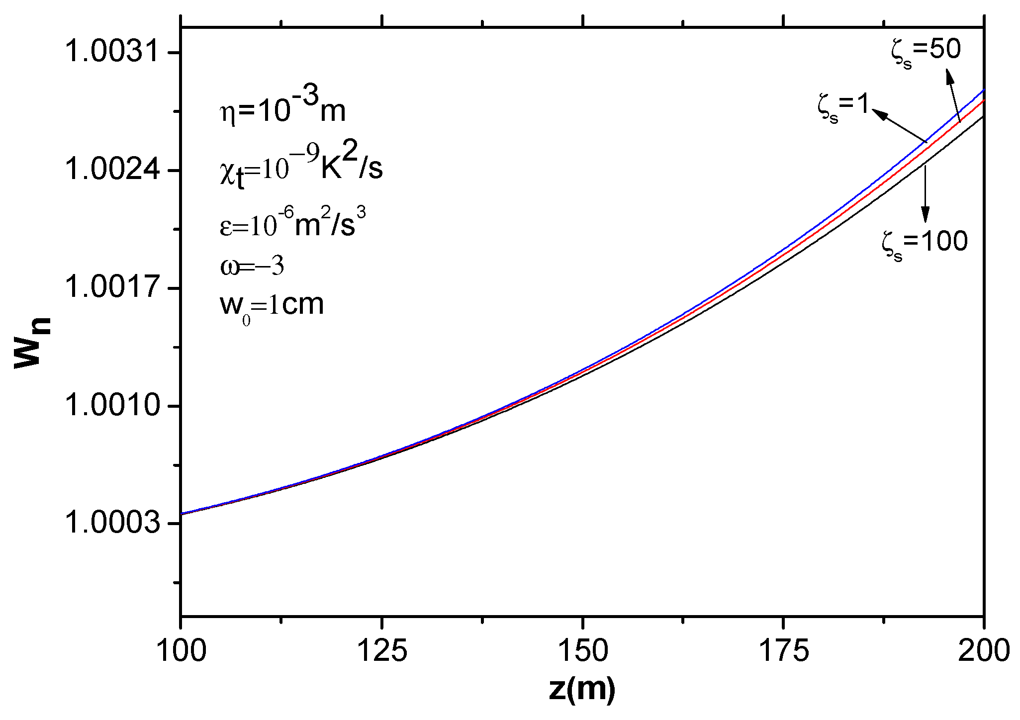
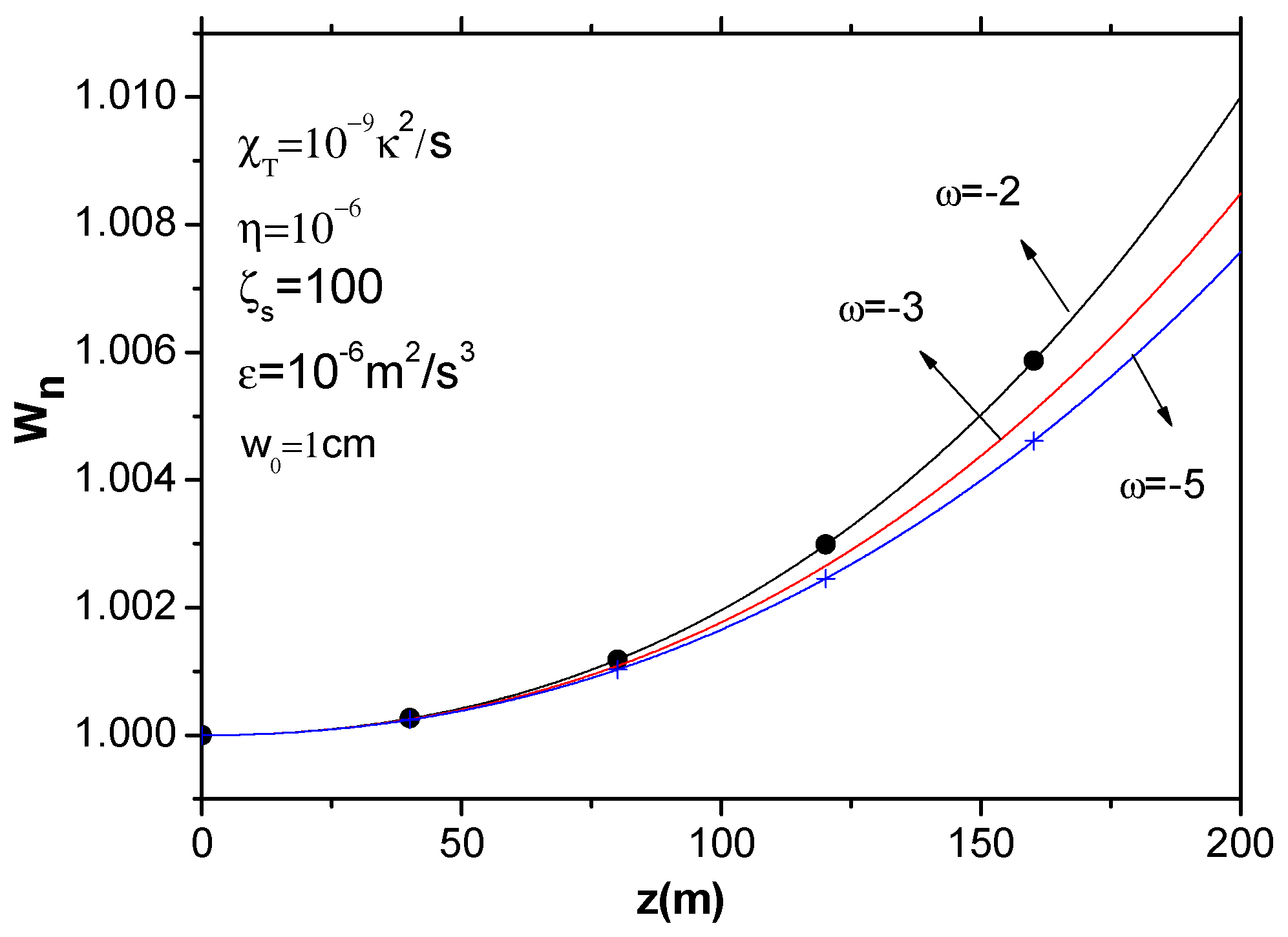
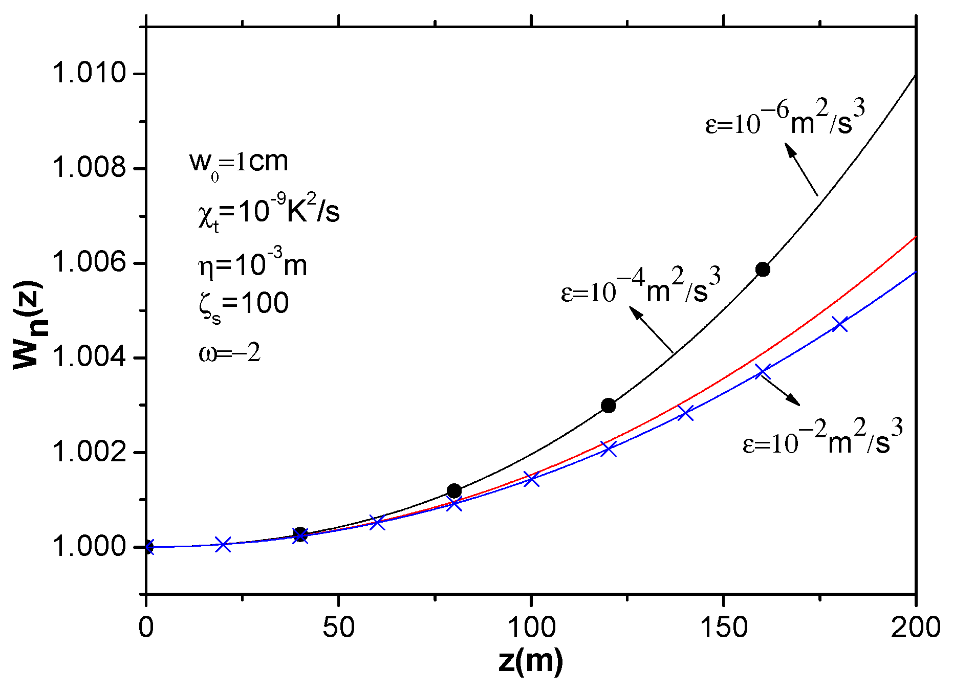
The corresponding relative mean-squared widths $W\left(z\right)/W_{\mathrm{f}ree}\left(z\right)$ of a GSM beam in turbulence and free space as a function propagation distance z for different values ${\zeta }_s$, $\omega$, and $\mathrm{\epsilon }$ are given in Figure 1, Figure 2 and Figure 3 based on $W_{\zeta }\left(z\right)=w_0({\mathsf{\Theta }}_0^2+\zeta {\mathsf{\Lambda }}_0^2{)}^{1/2}$. As shown in Figure 1, propagating 200 m through oceanic turbulence, the relative mean-squared width of a GSM beam (${\zeta }_s=100$) is 1.0025, and the relative mean-squared width of a coherent source beam (${\zeta }_s=1$) is 1.0027. It is demonstrated that a GSM beam is less sensitive to the effect of oceanic turbulence than the fully coherent beam, the same as in atmospheric turbulence [28]. While the propagation range is less than 150 m, the coherence effect is not evident. The simulation result of Ref. [20] uses a propagation length of 1000 m, which is not consistent with experimental research conducted at 200 m in deep oceans. In Figure 2, we specifically consider the role of oceanic turbulence by setting the source coherence parameter ${\zeta }_s=100$. When $\omega$ increases, i.e., if salinity dominates in oceanic turbulence, the relative mean-squared width increases. This is because salinity-dominated turbulence produces stronger refractive index fluctuations, which enhance scattering and lead to more dominant beam spreading. We plot and compare the spreading of the GSM beam for various values of $\epsilon$ in Figure 3. The result indicates that as the dissipation rate of turbulent kinetic energy per unit mass of fluid $\epsilon$ increases, the spreading of the beam will decrease. It is observed that the spreading is more pronounced with relatively stronger levels of turbulence. This is because stronger turbulence leads to larger refractive index fluctuations, which enhance the scattering of the beam as it propagates through different eddies. This result can be explained by the fact that the intensity of the turbulence becomes stronger when $\mathsf{\omega }$ increases or $\epsilon$ decreases.

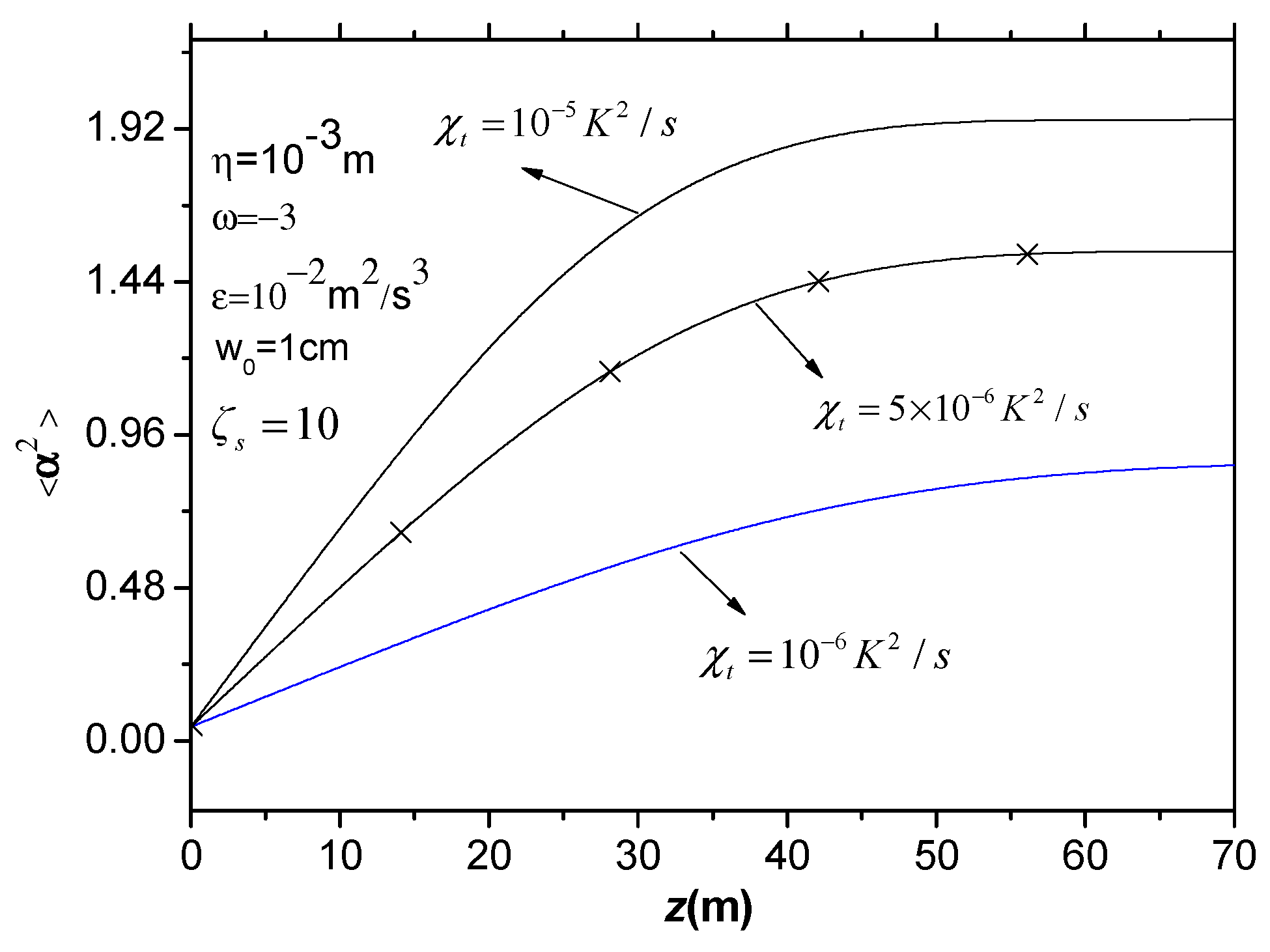
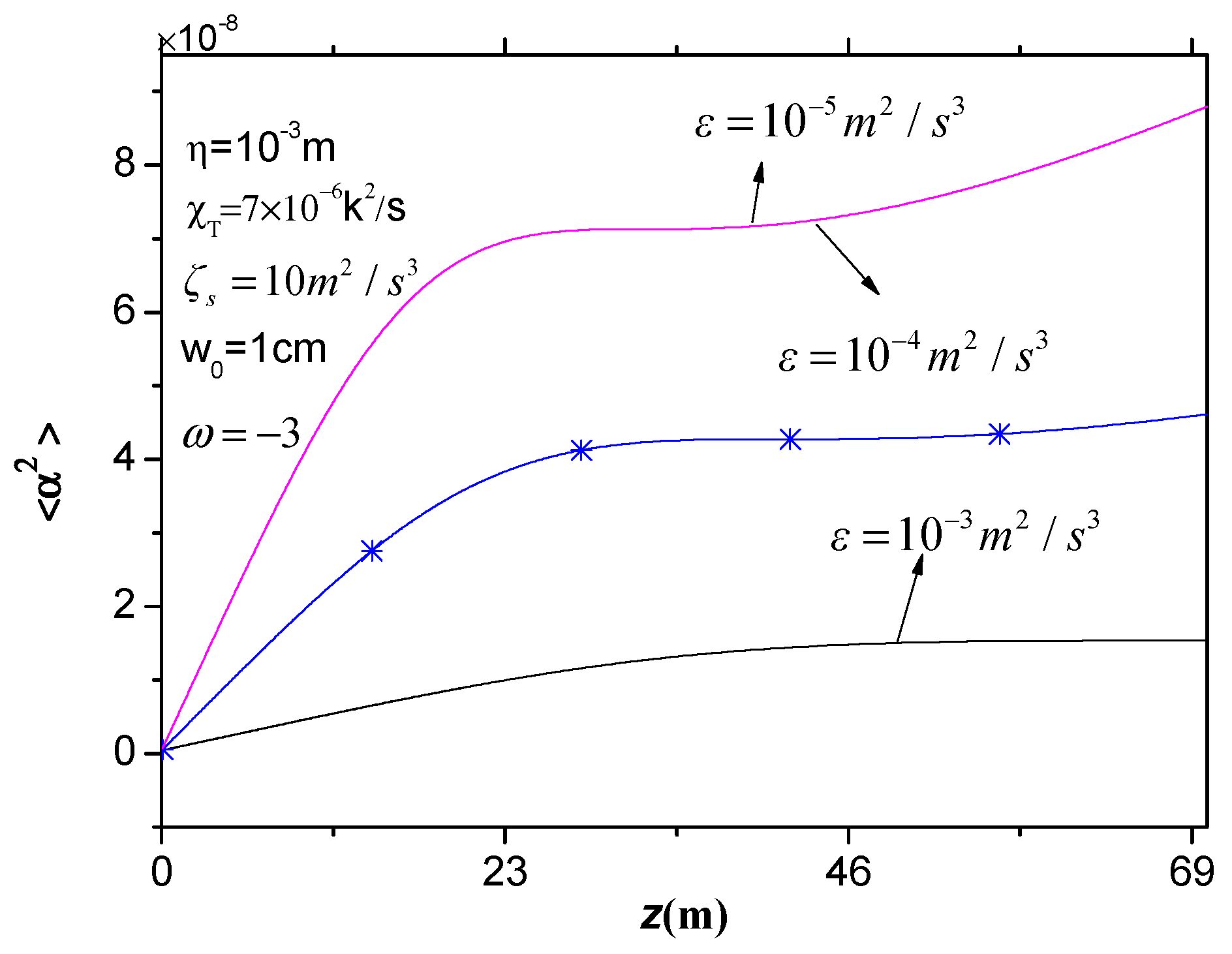
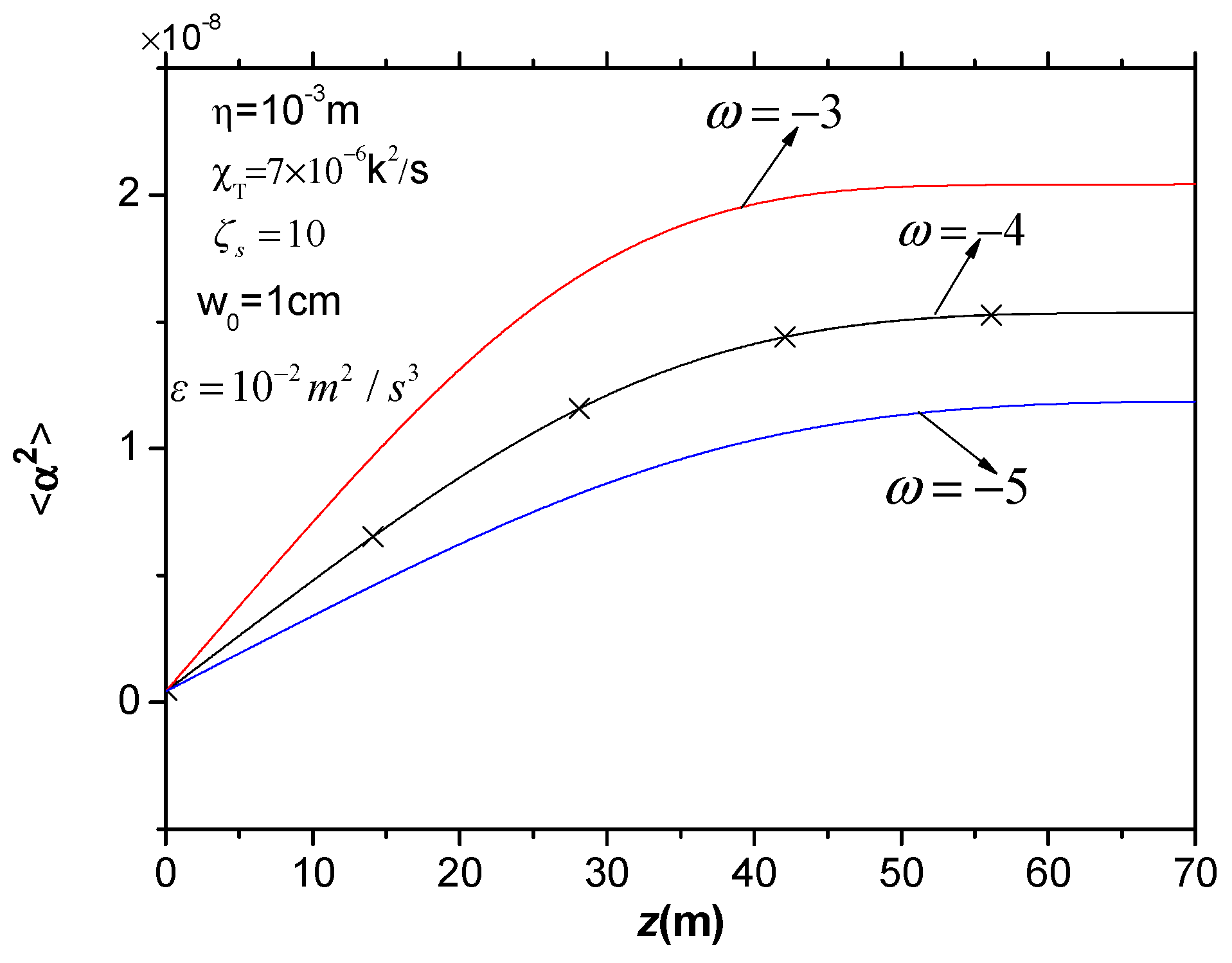
As shown in Figure 4, Figure 5 and Figure 6, on the basis of Equation (12), the angle-of-arrival fluctuation of the beam increases with increasing variables $z$. Figure 4 plots the angle-of-arrival fluctuation versus the ratio of temperature and salinity contributions to the refractive index spectrum. It can be seen that the bigger the temperature–salinity balance parameter $\omega$ is, the bigger the angle-of-arrival fluctuation. For each value of $\omega$, the angle-of-arrival fluctuation almost maintains a constant value when length exceeds 40 m. Physically, $\omega \to 0$, which produces stronger refractive index fluctuations and more severe phases front tilting, thereby increasing the angle-of-arrival fluctuation. From Figure 5, we derive the conclusion that the rate of dissipation of mean-squared temperature ${\chi }_t$ has a great influence on the angle-of-arrival fluctuation that actually occurs. ${\chi }_t={10}^{-6}{\mathrm{K}}^2/\mathrm{s}$, ${\chi }_t=5\times {10}^{-6}{\mathrm{K}}^2/\mathrm{s}$ and ${\chi }_t={10}^{-5}{\mathrm{K}}^2/\mathrm{s}$ are considered; when the value slightly increases, the angle-of-arrival fluctuation significantly increases with ${\chi }_t$. In Figure 6, the angle- of-arrival fluctuation is numerically calculated for several values of $\epsilon$; the angle-of-arrival fluctuation will increase with the rate of dissipation of turbulent kinetic energy per unit mass of fluid that $\epsilon$ decreases. The reason for this is that a large $\omega$ and ${\chi }_t$ and small $\epsilon$ mean strong turbulence, which will dominate the angle-of-arrival fluctuation. Note that as atmospheric turbulence strength $C_n^2$ increases, the angle- of-arrival fluctuation will increase [25].

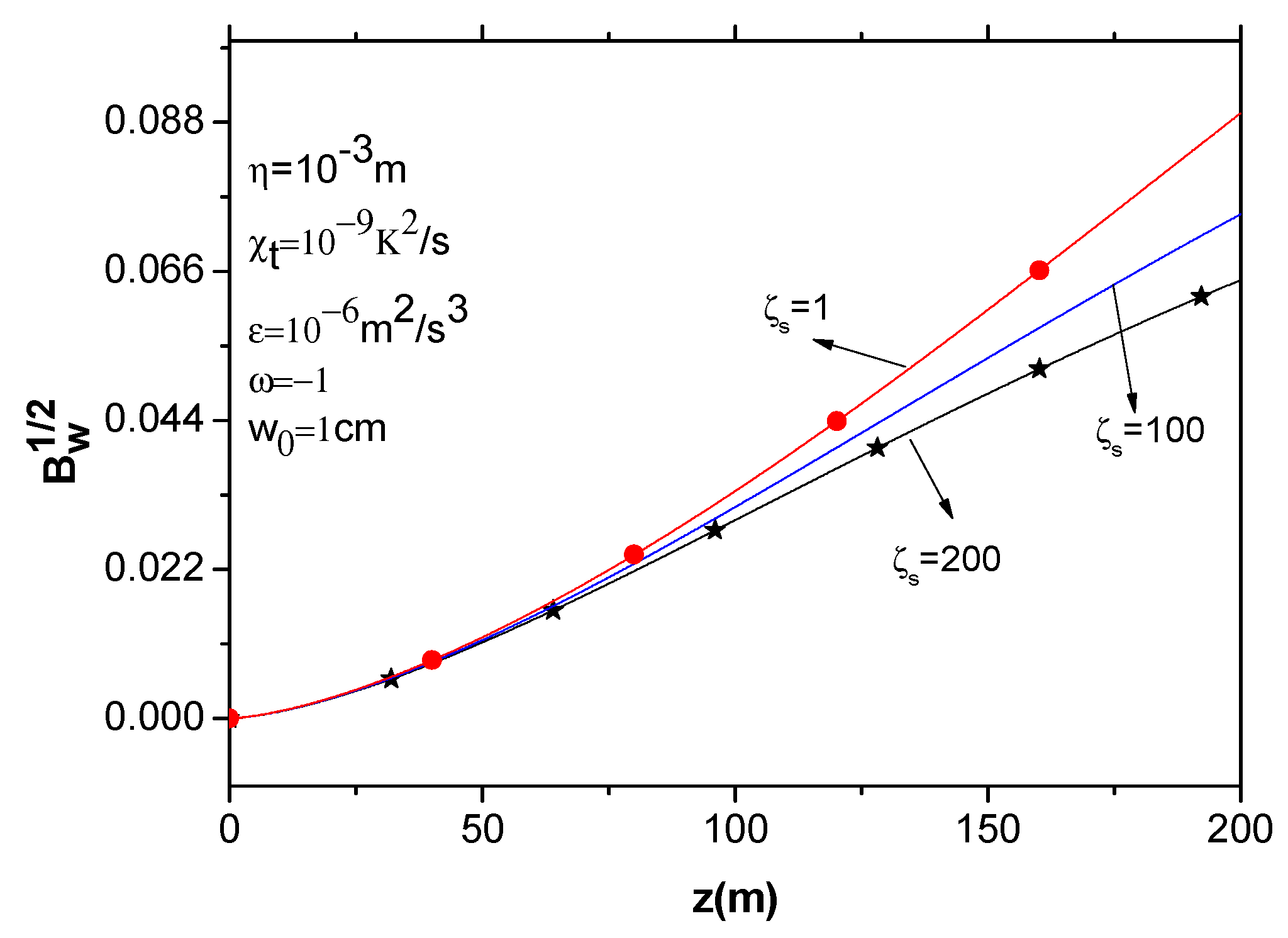
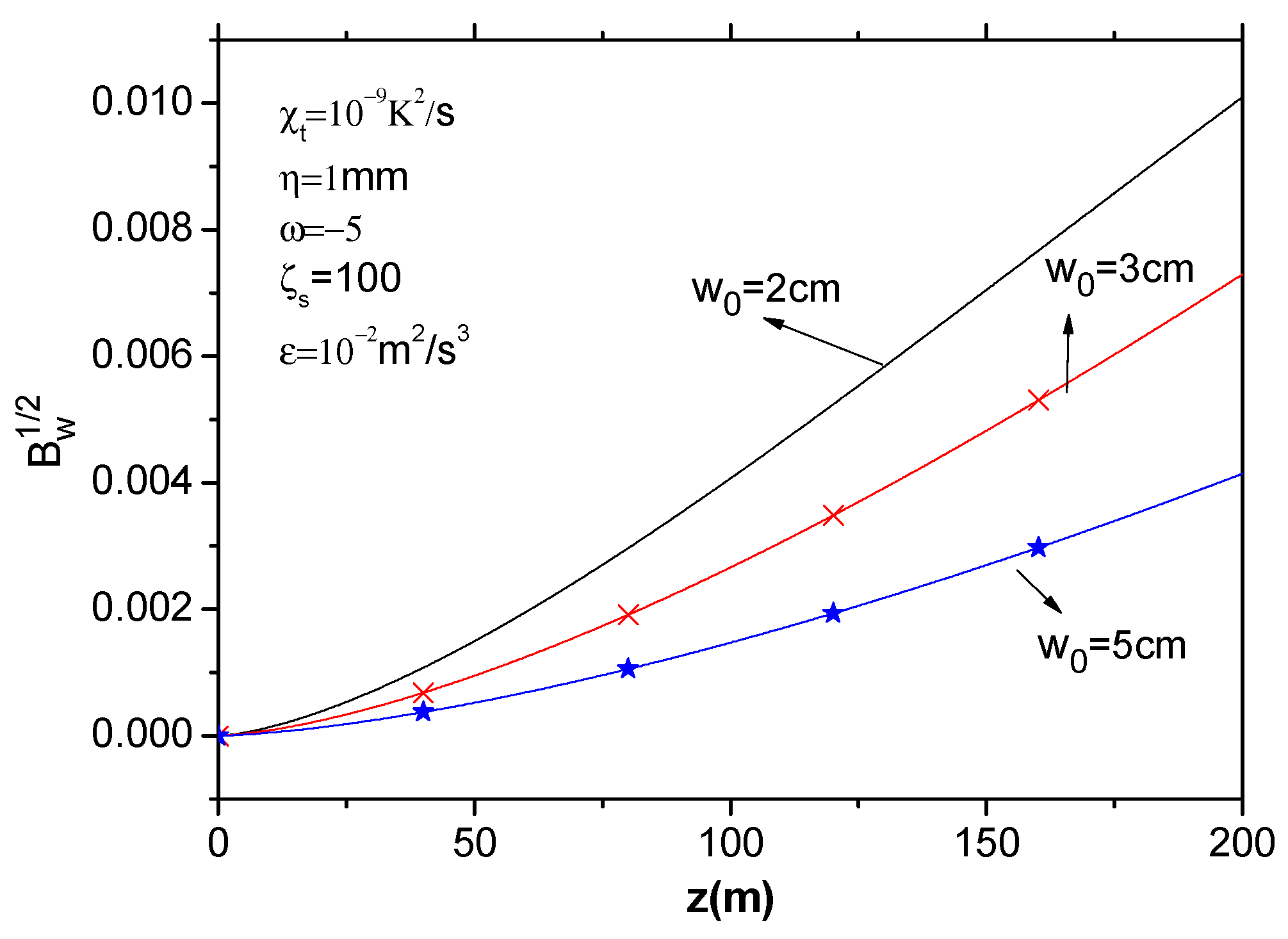
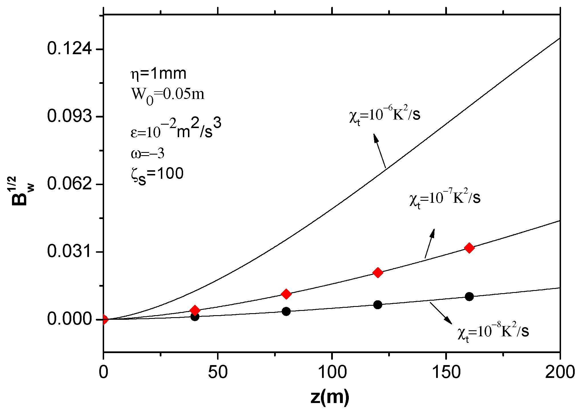
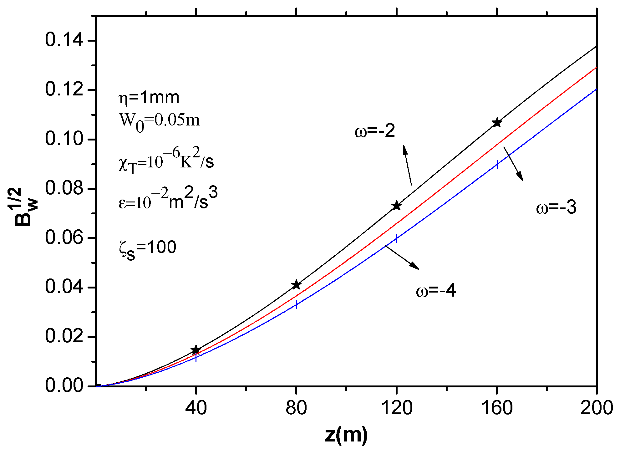
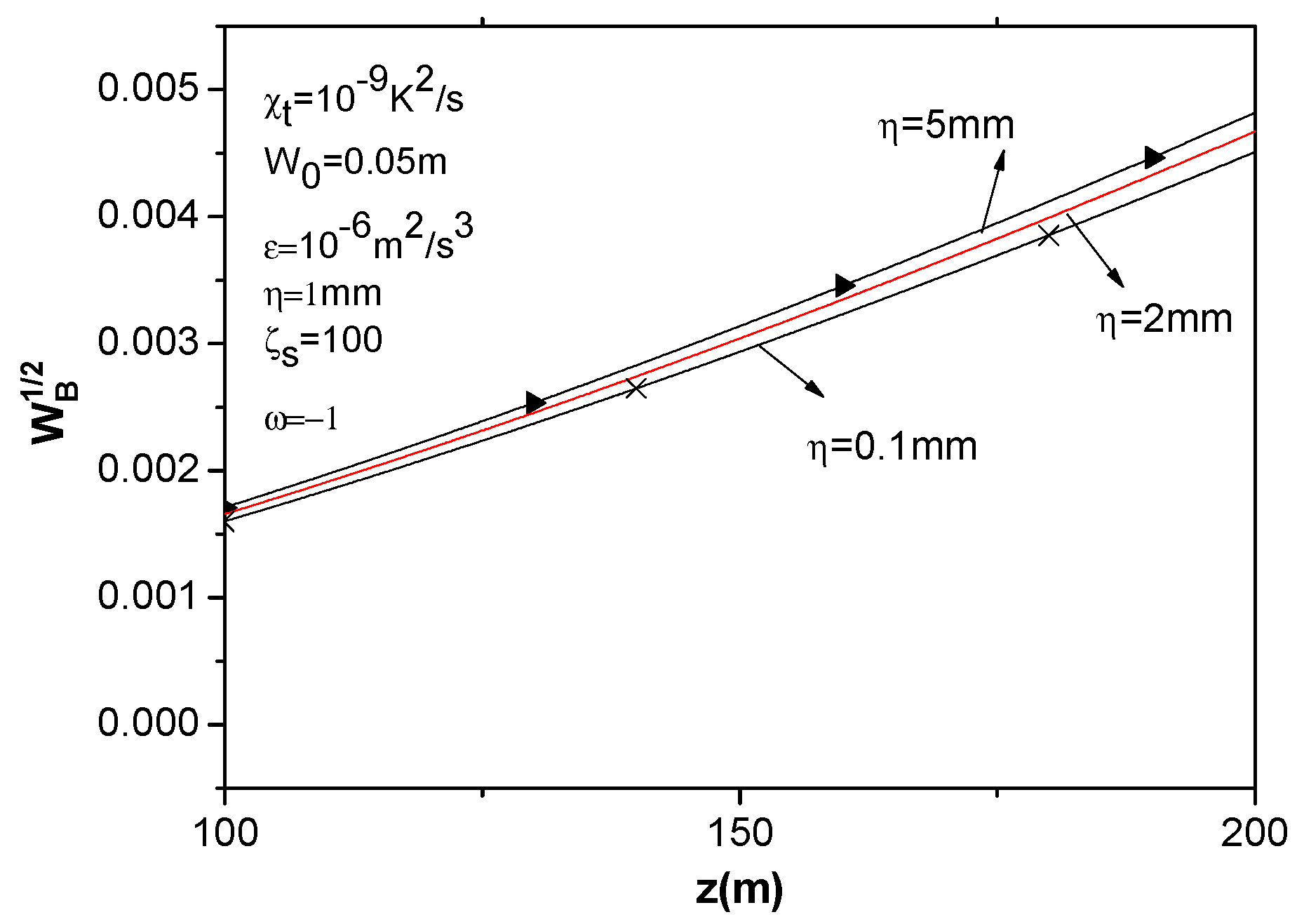
In Figure 7, Figure 8, Figure 9, Figure 10 and Figure 11, we consider the dimensionless quantity $B_W^{1/2}=\sqrt{〈r_c^2〉/W_{\zeta }^2}$, which is more informative than merely $〈r_c^2〉$ in the practical significance of the beam wander. From these figures, we can see that the beam wander increases with the propagation distance increase.

In Figure 7, we compare the wander behavior of the coherent beam (${\zeta }_5=1$) with that of the partially coherent beams (${\zeta }_s=100$, ${\zeta }_5=200$). As shown in Figure 7 the beam wander decreases as the source coherence parameter ${\zeta }_s$ increases. This indicates that partially coherent beam channels exhibit low beam wander. Thus, in practical applications, the reduction in the initial coherence of a partially coherent beam can be used to decrease the beam wander effect, which agrees well with Figure 4 in [19] and Figure 4 in [28]. Our result is also in accordance with the atmospheric turbulence case. The effect of partially coherent beams is less obvious for shorter propagation distances than for longer ones [29]. The reason is that increasing source coherence parameter ${\zeta }_s$ reduces spatial coherence, which averages out turbulent phase distortions and reduces beam wander.

As can be seen in Figure 8, the beam wander can be decreased by increasing the initial radius w₀ in oceanic turbulence. The larger the beam radius, the smaller the beam correlation when the light at different positions passes through the turbulence, which leads to the decrease in beam wander. The effect of the dissipation rate of temperature variance ${\mathrm{\chi }}_t$ on the wander is illustrated in Figure 9. As ${\mathrm{\chi }}_t$ becomes smaller, the beam wander decreases as expected. When the propagation length increases, this phenomenon becomes obvious. This behavior can be explained by the fact that the larger dissipation rate of temperature variance ${\mathrm{\chi }}_t$ means stronger turbulence. In atmospheric turbulence, the wander increases with increasing atmospheric turbulent structure parameter, which is similar to ${\mathrm{\chi }}_t$ in oceanic turbulence.

The beam wander of a GSM beam as a function of the propagation distance with three $\mathsf{\omega }$ is shown in Figure 10. The figure shows that the smaller parameter $\mathsf{\omega }$ has a weaker wander effect on oceanic turbulence. The parameter $\mathsf{\omega }$ can vary in the interval [−5; 0] for the ocean and refers to the dominating temperature and salinity-induced optical turbulence, respectively. The conclusion that salinity fluctuations have a greater impact on beam wander than temperature fluctuations is consistent with Wu et al. [18], who reported the same finding for GSM beams in oceanic turbulence. Physically, salinity-dominated turbulence produces a steeper high-wavenumber spectrum, enhancing small-angle scattering and thus beam wander.

The effect of the inner scale on the beam wander of turbulence is shown in Figure 11. For propagation distances $z<100\hspace{0.33em}\mathrm{m}$, the beam wander curves for different inner scales (η = 1 mm, 5 mm, 10 mm) are nearly 0.0017, but for a large link ($z>100\hspace{0.33em}\mathrm{m}$), the three curves are not in the same values depending on the turbulence inner scale. Wander is caused mostly by large-scale turbulence near the transmitter, and for that reason, the diffraction effects are not obvious.

In comparison with previous work, our results (Figure 8 and Figure 10) for beam wander are consistent with Yang et al. [19] and Andrews & Phillips [28] in that increasing the emitting beam radius w0 reduces beam wander, but they increase as the dissipation rate of temperature variance ${\chi }_t$ and the inner scale of turbulence $\mathsf{\eta }$ increase beam wander. The beam wander of a fully coherent Airy beam is generally higher than that of a partially coherent one in Ref [20]. In Figure 7, at z = 200 m, our GSM beam with ${\mathsf{\zeta }}_{\mathrm{s}}=100$ exhibits a beam wander value of 0.066, which is approximately 25% lower than that of a fully coherent beam ${\mathsf{\zeta }}_{\mathrm{s}}=1$. Our results are consistent with Ref [20].

The present analysis employs the paraxial approximation inherent to the extended Huygens–Fresnel principle, while future work can extend this study to anisotropic oceanic turbulence, experimental validation, and absorption and scattering effects for practical underwater wireless optical communication systems.

5. Conclusions

In summary, we propose a novel methodology to simulate the beam spreading, angle-of-arrival fluctuation, and beam wander of GSM beams propagating through an oceanic turbulent medium. The derived analytical expressions are obtained using the effective beam parameter method, and they reduce to the corresponding diffraction expressions under the assumptions of full coherence and the absence of turbulence. Numerical simulations show that the beam spreading, angle-of-arrival fluctuation, and beam wander of GSM beams all increase with the propagation distance. Our results indicate that oceanic turbulence has a weaker effect on partially coherent beams than on fully coherent Gaussian beams. In addition, the beam spreading, angle-of-arrival fluctuation, and beam wander of partially coherent GSM beams in oceanic turbulence are mainly caused by salinity fluctuations rather than temperature fluctuations in $\omega$. At z = 200 m, the relative mean-squared width increases by about 0.02% when ω changes from −5 (temperature-dominated) to −2 (closer to salinity-dominated) (see Figure 2). As shown in Figure 4, the angle-of-arrival fluctuation is significantly larger under salinity-dominated conditions (ω = −3) than under temperature-dominated conditions (ω = −5) at z = 70 m. The beam wander for $\omega =-2$ is 0.13, approximately 18% larger than that for ω = −4 is 0.11 (Figure 10).

Furthermore, the beam wander and angle-of-arrival fluctuation increase with the rise in mean-square temperature dissipation rate ${\mathrm{\chi }}_{\mathrm{t}}$ and the fall in turbulent kinetic energy dissipation rate per unit mass $\epsilon$. The inner scale of ocean turbulence has almost no influence on the beam wander. These results are useful for us when choosing the proper beam parameter in high-speed underwater optical communications.