Article

Research on Space-Time Data Prediction Model of Quantum Long Short-Term Memory Network Fusion

Institute of Quantum Information Technology, China National Institute of Standardization, Beijing 100191, China
*
Author to whom correspondence should be addressed.
Photonics 2026, 13(5), 477; https://doi.org/10.3390/photonics13050477
Submission received: 31 March 2026 / Revised: 6 May 2026 / Accepted: 8 May 2026 / Published: 11 May 2026
(This article belongs to the Special Issue Recent Progress in Quantum Communication)

Abstract

This study proposes a novel hybrid prediction model (QGCN-LSTM) that combines Quantum Graph Convolutional Networks (QGCN) with classical Long Short-Term Memory (LSTM). The model takes space-time data as input and employs a hierarchical graph-based quantum encoding strategy. Specifically, classical spatial features are first aggregated into critical regional hubs, which are then mapped into the Hilbert space through a dense quantum encoding layer. Multi-scale features are extracted through the collaborative computation of QGCN and quantum gated recurrent units, and a quantum attention module is introduced to dynamically screen key information. Finally, the prediction results are generated through quantum measurement and a classical output layer. In the space-time data prediction task of urban traffic flow, a benchmark model system covering classical, cutting-edge, and traditional architectures was constructed. The experimental results show that QGCN-LSTM utilizes quantum entanglement gates to establish non-local road network associations, dynamically allocate feature weights to enhance the impact of critical time steps, and achieves deep compression of lines through quantum line pruning technology, effectively alleviating the common problem of “poor plateau” in quantum neural network training. In terms of prediction accuracy, the mean absolute error (MAE) of its key hub nodes is reduced by 34.1% compared to the graph convolution LSTM (GCN-LSTM) model, and the Spatial Correlation Index (SCI) is improved to 0.89. In addition, it also shows excellent performance in dynamic response, edge computing efficiency, and other aspects, meeting the real-time requirements of the traffic signal control system. This study provides an effective paradigm for the application of quantum collaborative architecture in complex spatiotemporal prediction tasks.

1. Introduction

Space-time data prediction, as one of the core tasks of data analysis, has important application value in fields such as meteorological forecasting [1], financial market analysis [2], and industrial equipment monitoring [3,4]. Although the classical LSTM network excels at modeling long-term dependencies [5,6,7,8], it faces three fundamental limitations in modern prediction tasks: (1) gradient vanishing in deep architectures restricts convergence [9]; (2) computational complexity ( O n 2 for spatial features) impedes real-time inference; (3) limited capacity to extract high-dimensional features from complex systems such as climate evolution or financial fluctuations [10,11].
In recent years, Quantum Neural Networks (QNNs) have been proven to require fewer parameters than classical networks for capturing long-range nonlinear dependencies through quantum parallelism and exponential Hilbert space representation, providing a new computational paradigm for space-time data prediction [12,13,14,15]. The superposition and entanglement properties of quantum bits endow quantum algorithms with natural parallel processing capabilities [12], while high-dimensional state representations in Hilbert space can effectively capture nonlinear features that classical models find difficult to analyze [13].
Specifically, the core advantages of QNN for temporal prediction are reflected in three aspects: (1) parallel temporal processing: quantum circuits can process all time steps in one evolution, overcoming the time-consuming drawback of RNN/LSTM that must be sequentially unfolded; (2) Exponential representation capability: n qubits can encode 2n-dimensional states, naturally suitable for high-dimensional, nonlinear, high noise traffic flow and other scenarios; (3) parameter efficiency: VQC models often achieve comparable predictive performance with fewer trainable parameters than LSTM, thereby lowering implementation complexity on NISQ devices [14,15].
Recently, hybrid architectures that combine Feedforward Neural Network (FNN) with recurrent structures have been proposed to leverage both static nonlinear mapping and temporal memory. A representative example is the FNN-LSTM architecture [16], where an LSTM module first encodes the sequential dependencies and a subsequent FNN performs feature fusion and final prediction. This design has demonstrated improved accuracy in energy-load forecasting by explicitly separating temporal modeling from nonlinear transformation. Additionally, self-similar neural networks—networks whose components exhibit scale-invariant properties—have been explored to capture multi-scale temporal patterns without significantly increasing parameter count [17]. These studies reinforce the importance of jointly modeling short-term fluctuations and long-term trends, a principle that motivates our quantum-classical hybrid approach.
Based on this, this study proposes a novel hybrid prediction framework that integrates quantum computing and LSTM, aiming to break through the performance bottleneck of traditional models. Reconstructing the gating mechanism of LSTM using Variational Quantum Circuits (VQC), simulating the dynamic evolution of memory states through quantum rotation gates and controlled gate operations, and alleviating the problem of gradient vanishing. Design a quantum convolutional layer (QCNN) for multi-scale spatial encoding of input space-time data, combined with a quantum attention module to dynamically allocate feature weights and enhance the impact of critical time steps, and improve the joint modeling ability of long-term trends and short-term fluctuations. We introduce a quantum natural gradient descent algorithm to optimize parameter updates and design a quantum Dropout mechanism to suppress overfitting, ensuring model robustness under NISQ device noise and resource limited conditions.
The core contributions of this article are comprehensively refined to highlight our methodological innovations and practical advantages, which can be summarized as follows:
Innovation in Architecture (Deep Quantum-Classical Fusion): We propose the QGCN-LSTM hybrid architecture that innovatively integrates quantum graph convolution (QGCN), quantized gated recurrent units, and quantum attention mechanisms. Unlike existing cascade models where early measurement destroys quantum coherence, our design maintains entangled spatiotemporal feature extraction within the quantum circuit until the final decoding step.
Innovation in Optimization (Hardware-Friendly and Gradient-Stable): We develop a quantum phase estimation-based activation function (QPE-Act) to solve non-linear gradient mapping in quantum circuits. Furthermore, we adopt quantum natural gradient descent (QNGD) to overcome barren plateaus and accelerate convergence, and propose a novel regularization mechanism combining quantum Dropout with dynamic gate pruning to ensure lightweight deployment on NISQ devices.
Demonstrated Advantages (Accuracy, Robustness, and Efficiency): In the urban traffic flow prediction task, QGCN-LSTM demonstrates three significant advantages: (1) Superior predictive performance, significantly reducing MAE and improving the Spatial Correlation Index (SCI); (2) Extreme fault robustness, utilizing quantum state correlation to maintain high prediction accuracy even under 30–50% random sensor masking; and (3) Edge computing efficiency, exhibiting low latency and low energy consumption, offering a highly practical paradigm for real-time applications on resource-constrained platforms.

2. Related Work

2.1. Classical Neural Network Approaches

To break through the assumption limitations of statistical models on linear relationships, deep learning techniques emerged as a transformative solution. Recurrent neural networks (RNNs) and their improved variants, long short-term memory networks (LSTMs) and Gated Recurrent Units (GRUs), have significantly improved predictive performance due to their ability to model long-term dependencies through gating mechanisms [18,19,20,21]. However, the classic LSTM model still has inherent flaws. The vanishing gradient problem in deep network training restricts the convergence efficiency of the model, and the high computational cost caused by massive parameters hinders its deployment in resource constrained scenarios.

2.2. Hybrid Classical Models

Facing multi-scale spatiotemporal features, a single LSTM is difficult to balance spatial feature extraction and temporal dynamic modeling. To optimize the above problems, attention mechanisms have been introduced into temporal models, such as the Attention LSTM architecture, which strengthens the feature weights of key time steps through a multi factor feature dynamic weighted fusion layer. This can automatically focus on important time steps in temporal data, making it more effective in handling long-term dependencies [22,23]. Although this kind of scheme alleviates the defects of a single model, it is still limited by the bottleneck of classical computing power and is difficult to meet the demand for real-time prediction.

2.3. Quantum Approaches

The rise of quantum computing provides new ideas for solving the computational bottleneck of classical models. In specific algorithmic scenarios, quantum neural networks (QNNs) utilize quantum superposition and entanglement properties to achieve significant extensions in the state space dimension compared to classical networks, potentially providing richer representation capabilities when processing high-dimensional data [24]. Recent research has focused on two primary architectures: one is the quantum hybrid model, such as the Quantum Convolutional Long-Short Term Memory Network (QCNN-LSTM), which delegates spatial feature extraction to quantum convolutional layers (QCNN) while processing temporal dependencies through LSTM [25]. However, this cascaded design suffers from quantum information collapse: quantum measurements after the QCNN layer destroy coherent phase information before temporal processing, fundamentally limiting its ability to model entangled spatiotemporal correlations (e.g., dynamic road network interactions). In comparison, classical graph-based methods such as the Graph Attention Network (GAT) can also capture non-local dependencies through adaptive neighborhood aggregation, and therefore serve as an important baseline for evaluating space-time modeling performance. The second is the fully quantum gated architecture recurrent neural network (QGRNN), which uses parameterized quantum circuits to simulate classical gated units, rigorously proves the model’s immunity to long-term dependency problems through unitary evolution characteristics, and verifies gradient stability in gene regulation network prediction [26]. While effective for small-scale tasks like gene regulation networks (typically < 10 nodes), these models face severe scalability constraints: the GCN-QCNN-LSTM variant requires circuit widths scaling linearly with node count ( O n qubits for n nodes), making implementations beyond 20-qubit road networks experimentally infeasible on current NISQ devices. It is worth noting that existing quantum space-time data prediction models still face scalability challenges: on the one hand, variational quantum circuits become rapidly complex as the input data dimension increases, which can easily fall into the “barren plateau” dilemma, where parameter space gradients disappear [27]; On the other hand, although multi head quantum self attention models (such as MQSAPN) improve feature extraction efficiency by estimating attention coefficients through Gaussian functions, the balance between line depth and computational resource consumption has not yet been achieved. The current research trend indicates that the innovation of quantum fusion architecture needs to balance theoretical rigor and engineering feasibility. However, the exploration of spatiotemporal joint modeling in existing fusion schemes is still insufficient, and there is a lack of lightweight design for NISQ devices with noise, which is precisely the breakthrough direction of this study.
Recent studies have shown that Quantum Kernel Learning (QKL) can effectively capture non-linear structures in time-series classification and regression tasks by leveraging quantum feature maps [28]. In particular, QKL provides a promising alternative to variational quantum neural networks when the objective is to enhance separability in a low-dimensional latent space [29]. However, QKL typically relies on kernel-matrix evaluation, whose computational and memory costs may grow rapidly with the number of training samples. For spatiotemporal traffic forecasting, where the model must simultaneously capture graph-based spatial dependencies, temporal dynamics, and real-time inference constraints, an end-to-end architecture such as QGCN-LSTM is more suitable for our current setting. We therefore view QKL as a complementary direction that may be useful for smaller-scale forecasting or feature extraction tasks, while the proposed QGCN-LSTM remains focused on joint spatial-temporal modeling.
Beyond centralized forecasting architectures, the application of quantum neural networks has rapidly expanded into distributed, privacy-preserving, and security-critical prediction domains. For instance, in complex network environments, integrating Quantum Key Distribution (QKD) with quantum machine learning provides information-theoretic security for transmitting predictive data across nodes [30]. Furthermore, recent pioneering studies have explored Quantum Federated Learning (QFL) frameworks to enable decentralized predictive modeling [31]. By utilizing quantum circuits for local parameter training and aggregating quantum states or gradients globally, QFL ensures that raw spatiotemporal data (such as sensitive traffic or personal mobility trajectories) remains strictly on local devices while collaboratively training a robust global model [32]. Such advancements highlight the immense potential of quantum machine learning in distributed forecasting systems. While these distributed frameworks (e.g., QFL and QKD) excel in data privacy and secure communication, our proposed QGCN-LSTM model highly complements this ecosystem by focusing on the local node-level challenge: designing an efficient end-to-end quantum architecture capable of extracting highly entangled spatiotemporal features and mitigating barren plateaus on current NISQ devices.

3. Design of Quantum LSTM Fusion Model

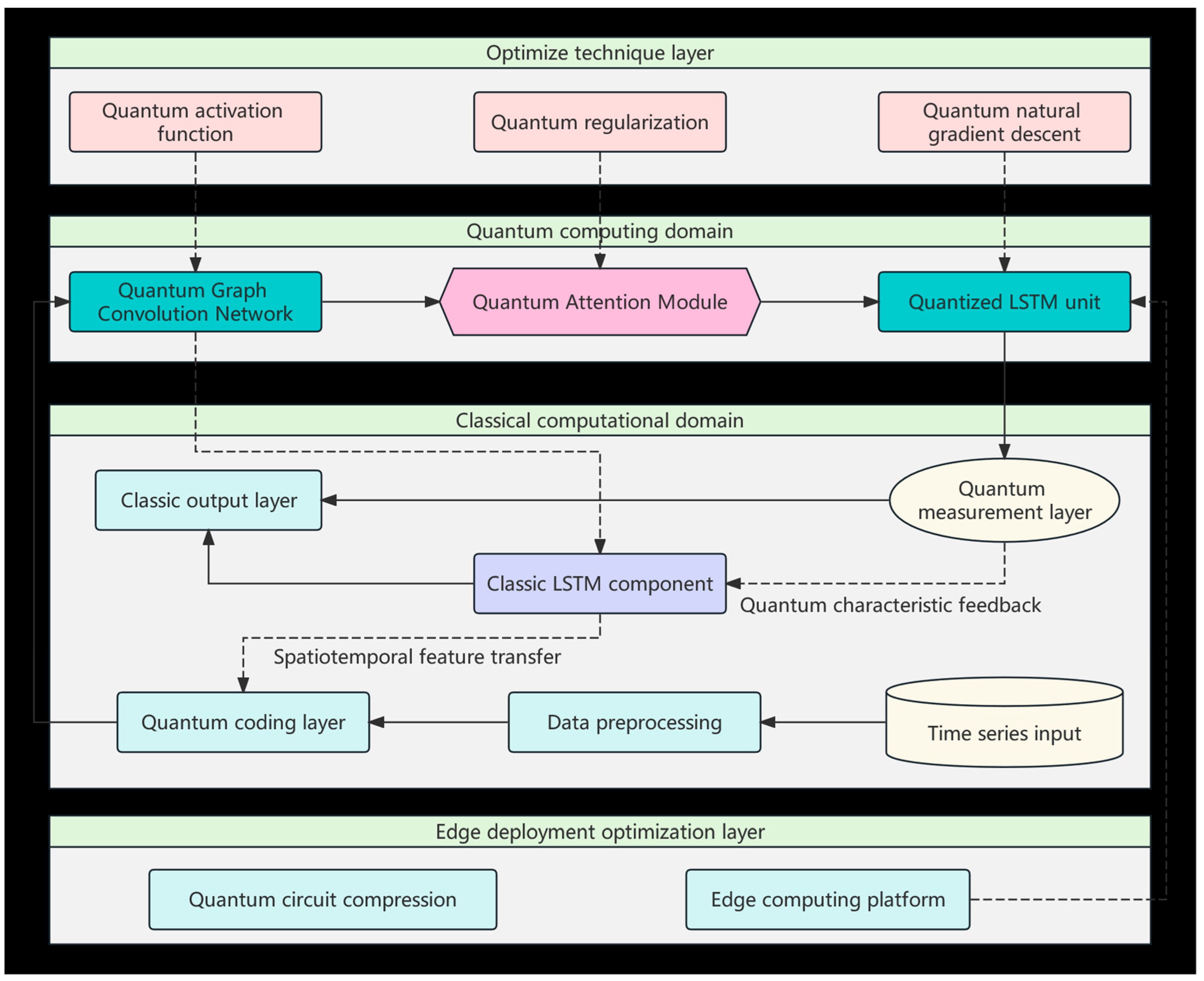
To build a prediction framework that combines quantum parallelism and classical temporal modeling capabilities, this study proposes a multi-level fusion architecture (as shown in Figure 1). This architecture takes space-time data as input, implements quantum information conversion through quantum encoding layers, extracts multi-scale features through collaborative computation of quantum convolution and quantized gating units, and finally generates prediction results through quantum measurement and classical output layers.

3.1. Quantum Encoding and Hybrid Computing Layer

To address the hardware constraints of NISQ devices while avoiding severe information loss when mapping large-scale spatial networks to a limited number of qubits, this study proposes a Local Subgraph Partitioning and Encoding strategy. Instead of forcibly compressing an entire global graph into a low-dimensional Hilbert space, the macroscopic space-time network is decomposed into overlapping local ego-networks (subgraphs).
For a target node i at time step t , we extract a local subgraph containing node i and its immediate topological neighbors, restricted to a maximum size of n nodes. The feature vector of this subgraph is denoted as x t R d ( d n ). The quantum encoding layer adopts an angle encoding strategy to map the classical features of these local nodes to the state vector of n qubits.
For the j -th node’s feature component in the subgraph j = 1,2 , , d , the rotation angle is computed through min-max normalization across all time steps:
θ j = π · x t j m i n x t j m a x x t j m i n x t j
where m a x x t j and m i n x t j denote the minimum and maximum values of the j-th feature observed over all time steps t in the training dataset.
Each quantum bit is initialized through a single qubit rotation gate operation, mapping one node’s feature to one specific qubit:
| ψ j = R y ( θ j ) | 0 = cos θ j 2 | 0 + sin θ j 2 | 1 = cos θ j 2 sin θ j 2
The Dirac notation | · denotes a quantum state vector (ket), where | 0 = 0 1 represents the ground state of a qubit. The encoded quantum state is | ψ t = j = 1 n | ψ j , and the original data is embedded into Hilbert space H C 2 n .
By iterating this process over all subgraphs in a batched manner, the model can process spatial networks of arbitrary scale without down-sampling or discarding critical spatial information. The hybrid computing layer consists of three core components: quantum convolution module (QCNN), quantized LSTM unit, and quantum attention module.

3.1.1. Quantum Graph Convolution (QGCN)

The entanglement operation ENTlinear establishes node correlations through CNOT gates applied only between topologically adjacent nodes:
U c o n v ( ϕ ) = k = 1 K i = 1 n R z ( ϕ k , i ) ( u , v ) E C N O T u v
where, E is the set of edges in the road network graph. This design ensures direct correspondence between quantum entanglement and spatial adjacency. For adjacent nodes ( u , v ) E : CNOT gates create entangled states; for non-adjacent nodes: No direct entanglement operation.
For each convolution depth k = 1 , , K and each qubit i = 1 , , n , ϕ k , i R is a trainable parameter applied via the rotation gate:
R z ( ϕ k , i ) = e x p i ϕ k , i 2 Z = e i ϕ k , i / 2 0 0 e i ϕ k , i / 2
The subscript i indexes the qubit; the subscript k indexes the depth layer. All R z gates at the same depth are applied in parallel. Algorithm 1 summarizes the construction of one QGCN layer.
Algorithm 1. Construction of one QGCN layer
Input:
latent quantum register q = q 1 ,   q 2 ,   ,   q d
learnable parameters ϕ k = ϕ k , 1 ,   ϕ k , 2 ,   ,   ϕ k , d
  ordered edge list E o r d = i 1 , j 1 ,   i 2 , j 2 , ,   i E , j E
Output:
convolution unitary   U c o n v ( k )
Step 1: for i = 1 to d do
apply R z ( ϕ k , i )   on   q i
end for
Step 2: for m = 1 to E do
apply CNOT with control q i m and target q j m
end for
Return:
                  U c o n v ( k )
The spatial interpretability is verified through Quantum Topological Fidelity (QTF):
Q T F ( u , v ) = T r ρ u ρ v ρ u 2 ( u , v ) E 0 o t h e r w i s e
where ρ u and ρ v denote the reduced density matrices of the quantum subsystems corresponding to nodes u and v , obtained by tracing out the rest of the global quantum state. This metric accurately quantifies the entanglement and state similarity between mixed states of local node subsystems.

3.1.2. Quantify LSTM Unit

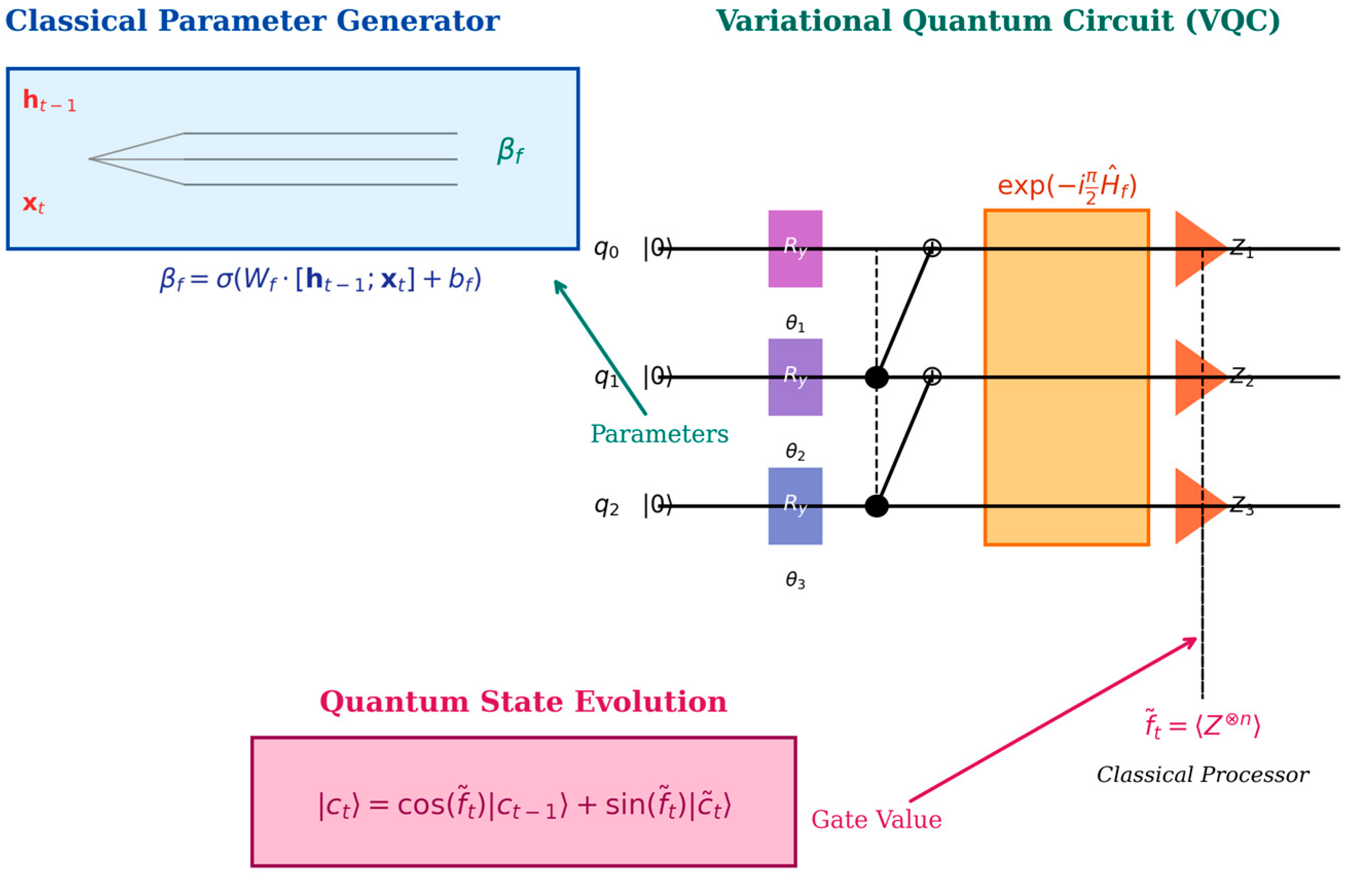
The gating mechanism of LSTM has been reconstructed into Variational Quantum Circuits (VQC). Taking the quantum forget gate as an example, its unitary operator is defined as:
U f h t 1 , x t = e x p i π 2 H ^ f β f
where, H ^ f = k = 1 M β f k P k is the linear combination of Pauli operators P k I , X , Y , Z n [33]. This design realizes the quantization reconstruction of the classical forget gate.
1.
Parameter generation mechanism
The parameter vector β f R M is generated by a lightweight classical fully connected neural network using the classical hidden state h t 1 and input x t :
β f = σ W f · [ h t 1 ; x t ] + b f
where, W f R M × d h + d x is the weight matrix, b f is the bias term, and σ is the Sigmoid activation function. This design enables quantum gating to dynamically respond to changes in spatiotemporal characteristics.
2.
Nonlinear function mapping
Quantum simulation of classical sigmoid functions is achieved through the combination of Pauli operators: Pauli operator bases {I, X, Y, Z} form SU(2) group generators, the eigenvalue spectrum of Hamiltonian H ^ f corresponds to the classical gating range [0, 1], and the exponential mapping e x p i π 2 H ^ f transforms the parameter space into a unitary group SU(2n).
3.
Quantum state evolution
This design transforms the nonlinear computation of LSTM gating functions into the unitary evolution of Pauli operator combinations in parameterized quantum circuits (VQC). Specifically, the function of the forget gate is implemented by the unitary operator U f , whose parameter β f contains gating information from the previous hidden state and the current input. The update of quantum memory cell states is achieved through controlled rotation operations:
| c t = c o s f ~ t | c t 1 + s i n f ~ t | c ~ t
where, the gate control value f ~ t = ψ c o n v | U f Z n U f | ψ c o n v is the expected value of the observable quantity Z after the forget gate effect, obtained through quantum measurement. f ~ t determines the retention ratio of the historical cell state | c ~ t 1 , while | c ~ t represents the current candidate cell state. This design has the following advantages:
(a)
Quantum parallelism
Utilize the parallelism of quantum operations to obtain global gating values in a single measurement.
(b)
High dimensional representation
By utilizing the high-dimensional representation capability of Hilbert space, n-qubit coverage of a 2n dimensional state space can be achieved, enabling more efficient simulation of the complex dynamics and gating mechanisms of cellular states. Consider n = 2 quantum bits example, constructing Hamiltonian:
H ^ f = β 1 Z I + β 2 I Z + β 3 Z Z
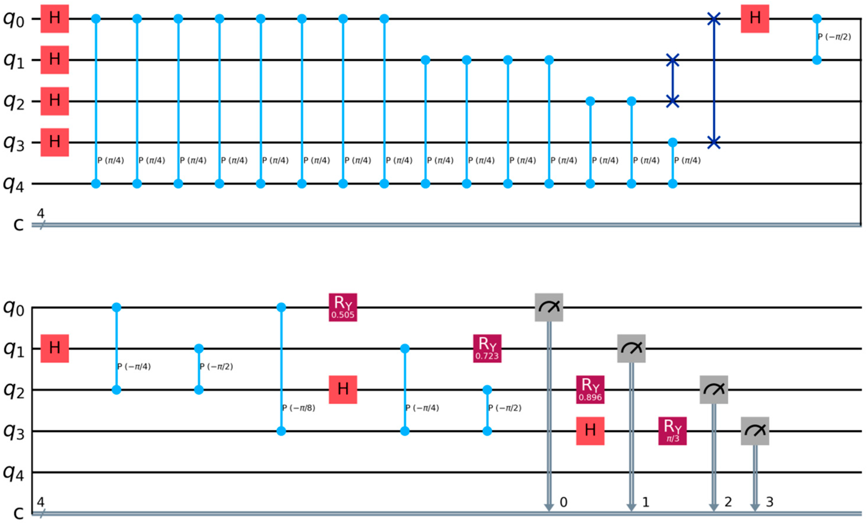
Quantum circuit implementation:
Photonics 13 00477 i001
There is an analytical mapping relationship between the rotation angle θ i , ϕ i and β f .
Gate control value measurement: f ~ t = Z Z reflects the two bit correlation state.
(c)
Differential continuity
Calculate gradient through parameter translation rule:
f t β k = 1 2 f t β k + π 4 f t β k π 4
Expected value measurement maintains parameter gradient traceability, potentially alleviating the gradient vanishing problem in deep LSTM.

3.1.3. Quantum Attention Module

Calculate time step correlation weights through quantum state fidelity:
α t , k = ψ c o n v t | ψ c o n v k 2 j = t T t 1 ψ c o n v t | ψ c o n v j 2 k t T , t 1
The weighted contextual state is | ξ t = k = t T t 1 α t , k | ψ c o n v k .
Finally, the quantum state information collapses into a classical probability distribution through Pauli Z-basis measurement, and is decoded by a fully connected layer to output the predicted value. The entire process forms a closed-loop computing path of “classical → quantum → classical”, balancing the advantages of quantum parallelism and classical interpretability. Figure 2 provides a detailed explanation of the internal structure of the quantum QLSTM unit.

3.2. Key Technology Implementation

3.2.1. Quantum Activation Function

The innovative design of quantum activation functions is the core of solving gradient problems. The classical ReLU function is difficult to directly implement in quantum circuits. This study proposes an activation mechanism based on quantum phase estimation (QPE Act): extract the phase information of the rotation gate’s output state and encode it into an auxiliary quantum bit register via quantum Fourier transform and the quantum phase estimation (QPE) algorithm, and the nonlinear characteristics of ReLU are simulated using phase truncation operation.
  • Mathematical Definition
Given a unitary operator U acting on the quantum state | ψ with an eigenvalue e i 2 π θ , we design a nonlinear activation based on quantum phase estimation (QPE-Act). The QPE algorithm first encodes the phase θ [ 0,1 ) into a p -qubit auxiliary register as an integer representation:
| 0 p | ψ Q P E | θ ~ | ψ , θ ~ θ 2 p
Subsequently, a nonlinear truncation operation simulating the ReLU function is applied to the auxiliary register:
f R e L U ( | θ ~ ) = | max ( 0 , θ ~ θ t h r e s h o l d )
Here, p is the number of phase precision bits determining the resolution of the nonlinear approximation, and θ t h r e s h o l d acts as the zero-point cutoff for the ReLU activation.
2.
Physical implementation process
As shown in Figure 3, QPE Act is implemented through three-level quantum circuits:
(a) Phase extraction: Use quantum phase estimation algorithm (QPE) to encode the expected value of Z n into auxiliary registers:
Q P E : | 0 p | φ m c ~ m | m | φ
where, | m stores the binary representation of phase values.
(b) Nonlinear transformation: performing controlled rotation operations in auxiliary registers:
R y 2 a r c s i n m / 2 p m = 1 m 2 p 0 + m 2 p 1
(c) Selective measurement: Measure the last quantum bit of the auxiliary register:
P r 1 = m c ~ m 2 · m 2 p R E L U Z n + 1 2

3.2.2. Parameter Optimization Strategy

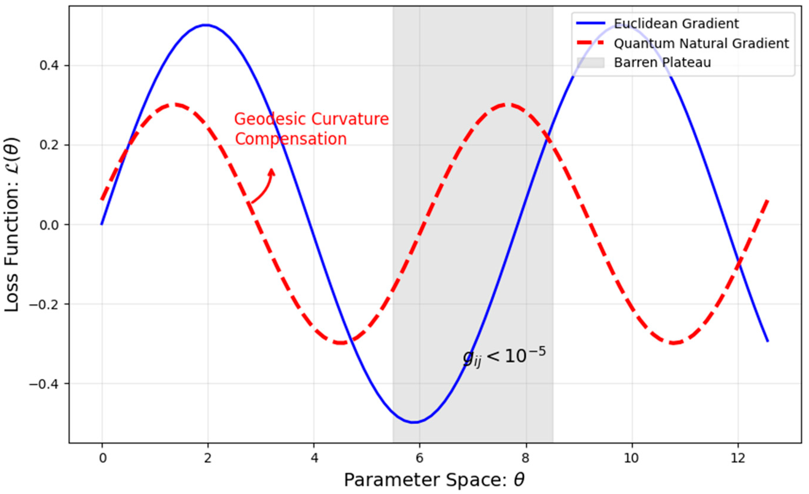
The parameter update adopts Quantum Natural Gradient Descent (QNGD) method. Unlike traditional stochastic gradient descent, QNGD incorporates the local geometry of the quantum state manifold through the Fubini–Study metric, thereby improving the conditioning of parameter updates [34,35] and, in some cases, mitigating optimization stagnation associated with barren-plateau-like landscapes. As shown in Figure 4, standard stochastic-gradient descent (blue solid curve) often stalls on a barren plateau, whereas QNGD follows the geodesic (red dashed curve) dictated by the Fubini–Study metric, yielding faster convergence in certain regimes.
To illustrate the mechanism, consider a toy example with two parameters θ = [ θ 1 , θ 2 ] and a raw gradient g = L = [ 0.1,0.2 ] . In Euclidean space, the update is proportional to g . If the QFIM is F = 2.0   0   0   0.5 , it indicates the quantum state is highly sensitive to θ 1 but less so to θ 2 . The inverse F 1 = 0.5   0   0   2.0 yields a corrected update direction F 1 g = [ 0.05,0.4 ] . This ensures that the step size is uniform relative to the actual change in the quantum state (fidelity) rather than the arbitrary parameterization.
For a comprehensive derivation of the QFIM for variational circuits, readers are referred to the work by Stokes et al. [36], which establishes the equivalence between QNG and the natural gradient in the limit of small learning rates.
However, recent studies have also highlighted important limitations of QNGD for barren plateau mitigation [37,38,39,40]. In particular, QNGD may alleviate—but does not fundamentally eliminate—barren plateau behavior, especially in deep or highly expressive ansätze. Moreover, estimating the quantum Fisher information matrix (QFIM), or equivalently the Fubini–Study metric, introduces additional circuit- and sampling-related overhead on NISQ hardware.
To address the practical cost of QNGD, we further measured the overhead of estimating g Q 1 for the proposed 8-qubit circuits on IBM Quantum hardware. In our implementation, the QFIM was approximated using finite-shot overlap measurements and then inverted classically with a regularized pseudo-inverse. For an 8-qubit circuit with P trainable parameters, the metric estimation required O P 2 pairwise overlap evaluations in the worst case, although symmetry and sparsity reduced the number of distinct measurements in practice. On IBM_perth, the average runtime for a single QFIM estimation step was 4.6 s, corresponding to 7000 shots and 70 additional circuit executions per optimization step. Compared with standard gradient-based optimization, QNGD increased per-step hardware cost by approximately 50%, but yielded faster convergence in the early training stage and improved stability under noisy gradients. These results indicate that QNGD is beneficial when optimization efficiency is prioritized, but its overhead must be carefully balanced against the available NISQ resources.
The scalability of the proposed quantum circuit must be considered in relation to the growth of the road-network size. As the number of intersections increases, the model may require additional qubits, more complex encoding schemes, and deeper entangling layers, all of which can increase circuit depth, training difficulty, and hardware resource requirements. In particular, larger circuits may exacerbate barren-plateau-like optimization issues and reduce trainability under NISQ constraints. Thus, the current QGCN-LSTM design is most appropriate for small- to medium-scale networks, whereas large-scale urban deployments will likely require circuit compression, subgraph partitioning, or hybrid quantum-classical decomposition.
  • Fundamentals of Riemannian Geometry
The quantized quantum state ψ θ forms a Riemannian manifold in the complex projective space C P N 1 N = 2 n . Fubini-Study measures the natural metric tensor on this manifold:
d s 2 = d ψ d ψ d ψ ψ ψ d ψ
where | d ψ = i | φ θ i d θ i . The degree specifies the infinitesimal distance of the quantum state space:
d F S | d ψ , | ϕ = a r c c o s ψ ϕ
2.
Quantum Fisher Information Matrix
The Fubini-Study metric is represented by a quantum Fisher information matrix in a parametric coordinate system:
g Q θ i j = R e ψ θ i ψ θ j ψ θ i ψ ψ ψ θ j
3.
Optimization mechanism and alleviation of barren plateau
The update rule of traditional gradient descent is:
θ k + 1 = θ k η L θ k
Quantum natural gradient introduces metric correction:
θ k + 1 = θ k η · g Q 1 θ k L θ k
The core mechanism for alleviating the barren plateau is:
(a) Curvature compensation: g Q 1 corrects the parameter update direction to make the path follow the manifold geodesic;
(b) Scale invariance: eliminating the influence of parameterization methods on optimization paths;
(c) Quantum parallelism: A single quantum state evolution can simultaneously compute all g i j elements.

3.2.3. Regularization Mechanism

To improve the generalization ability of the model on NISQ devices, this study proposes a bimodal quantum regularization scheme, quantum Dropout, and dynamic circuit pruning. Quantum Dropout randomly shields some quantum gate operations in the circuit (such as skipping CNOT gates with probability p), effectively reducing model complexity; Dynamic pruning evaluates the importance of Pauli’s expected value and removes quantum gates that contribute less than the threshold θ to the output. The two work together to suppress overfitting and reduce validation set loss in data prediction tasks.
  • Quantum Dropout Implementation
Quantum Dropout is implemented by randomly masking sub operations in the unitary operator, and its mathematical form is:
U d r o p = l = 1 L B l · U l + 1 B l · I B l ~ B e r n o u l l i p
where, p is the gate retention probability (default p = 0.7), L is the total number of layers in the line, and B l is the Bernoulli gating variable.
(a) Application strategy:
  • Quantum convolutional layer: Randomly skip 30% of CNOT entanglement gates.
  • Quantum LSTM: Dropout is applied to the rotation gates of the forget gate and input gate.
  • Quantum Attention: Controlled Phase Gates in Fidelity Computing.
(b) Spatial distribution:
P s k i p = 0.3 × e x p G r a d U l m a x G r a d
Ensure that gates with smaller gradient amplitudes have a higher probability of dropout.
2.
Fidelity impact and control
The fidelity attenuation introduced by quantum Dropout can be quantified as:
F d r o p = ψ i d e a l ψ d r o p 2 = l = 1 L p + 1 p ψ l ϕ l 2
where, | ψ l is the ideal output state, and | ϕ l is the equivalent state after the dropout operation.
The adaptive probability adjustment strategy is as follows:
p t = p 0 + 1 p 0 × t a n h t T d e c a y
In the early stage of training, p 0 = 0.5 , in the late stage, p t = 0.9 , and T d e c a y = 1000 steps.
Apply virtual rotation compensation to the discard door:
δ θ l = a r c s i n 1 F l o c a l p
where, F l o c a l = 0 U l U i d e a l 0 2 .
3.
Dynamic route pruning
Gate importance evaluation based on Pauli expectation gradient: The importance of each gate U l is quantified by I U l , calculated as:
I U l = L P i · P i θ l
Pruning rule: Based on the importance score from Equation (26), we generate a binary mask m l for each gate. The mask determines whether a gate is retained or removed:
m l = 1 I U l > θ 0 I U l θ
where θ is a predefined pruning threshold, set to 0.05 in our experiments. The final pruned architecture is obtained by applying these masks.
4.
Collaborative regularization effect
To synergize quantum Dropout with the pruning process, we introduce a collaborative regularization term into the effective loss function. This term leverages the importance score I U l from Equation (26) to penalize gates that are both low-importance and have a large magnitude, thereby encouraging the model to learn a sparse structure during training.
The effective loss R e f f is formulated as:
R e f f = E B L L 0 + λ l = 1 L 1 I U l · W l F r o
where, E B L L 0 represents the loss function offset caused by Dropout, λ is the collaborative regularization strength coefficient ( λ > 0), and W l F r o is the Frobenius norm of the trainable parameters W l associated with gate U l .

4. Experiments and Results

To verify the universality of the quantum LSTM fusion model in complex spatiotemporal prediction tasks, this study selects urban traffic flow prediction as a typical application scenario.

4.1. Experimental Setup

The experiment was deployed on a hybrid quantum-classical platform, where the classical computing unit used an NVIDIA Jetson AGX Orin edge device and the quantum module was implemented using IBM Quantum’s 7-qubit superconducting backend IBM_perth for hardware validation of representative subcircuits. The full QGCN-LSTM model is designed with n = 8 qubits, which enables encoding of the 138-node road-network features and provides one auxiliary qubit for the quantum phase activation function (QPE-Act). Hardware validation was performed by decomposing the model into two representative sub-circuits whose combined widths do not exceed the 7-qubit limit: A 4-qubit QGCN layer, representing the core spatial feature extraction module of the model; and A 3-qubit QNGD parameter update step, corresponding to a key optimization phase of the model. These two sets of sub-circuits collectively utilize 7 qubits, strictly matching the physical resources of IBM_perth. Each hardware execution involves measuring the output fidelity and execution latency, with statistics obtained from 1024 shots. Table 1 summarises the gate counts and average error rates for the configurations evaluated on the real device.
The dataset consists of dynamic traffic monitoring records collected from a city in southwestern China from January to June 2023. It contains 5-min-resolution flow, speed, and occupancy measurements from 7500 detectors distributed over 138 key road-network nodes. Data preprocessing includes min-max normalization on each feature channel and spatiotemporal interpolation for a small number of missing values. This dataset presents three typical characteristics:
(1) spatial correlation, the road network topology forms 138 key nodes, and the traffic correlation coefficient between adjacent nodes reaches 0.78 ± 0.12;
(2) multi-periodic temporal patterns, including daily rush-hour cycles and weekly weekday/weekend differences, further perturbed by meteorological events; and
(3) abrupt nonstationary fluctuations, where accident-induced congestion may reach up to 4.2 times the steady-state traffic flow.
To address the limited qubit capacity of current NISQ hardware, the proposed model does not directly encode the full 138-node road network into 8 qubits in a one-to-one manner. Instead, we adopt a hybrid dimensionality-reduction and block-encoding strategy, in which the original large-scale graph signal is first compressed classically and then mapped into a low-dimensional quantum latent space.
At each prediction time step, the 138-node graph, where each node contains three traffic attributes, is first fed into a classical graph aggregation module that performs topology-aware feature compression through adjacency-guided pooling, producing a compact latent representation that preserves the key dynamic characteristics of the traffic network, including the dynamics of major hub nodes, the interactions among first-order neighbors, and the dominant global traffic modes.
After this classical preprocessing stage, the original node-level feature tensor is transformed into an 8-dimensional latent vector, which is then encoded into an 8-qubit quantum register through angle encoding. Therefore, the 8 qubits represent a compressed spatiotemporal embedding of the traffic network rather than a lossless encoding of all 138 nodes.
This design is motivated by current hardware constraints and should be interpreted as a low-dimensional quantum feature transform on graph summaries, not as a full quantum representation of the entire road network. The purpose of the quantum module is to enhance nonlinear correlation modeling in the compressed latent space, while the large-scale graph structure is primarily handled by the classical front-end.
The graph compression stage begins by ranking nodes according to a composite centrality score that combines traffic-flow variance, degree centrality, and betweenness centrality, after which the network is partitioned into functional traffic regions centered on major hubs. At each time step, local node features are then aggregated within these regions to construct a reduced graph-level representation, while several global descriptors, including the network-wide mean flow, congestion dispersion, and occupancy variance, are appended to preserve coarse-scale system dynamics. Consequently, the final latent vector used for quantum encoding is 8-dimensional, consisting of four dimensions obtained from regional hub-centered aggregation, two dimensions from inter-region interaction summaries, and two dimensions from global traffic statistics, so that the quantum encoding stage operates on the compressed representation z t R 8 rather than the original raw graph signal X t R 138 × 3 .
This compression mechanism substantially reduces the required circuit width and enables deployment on current small-scale quantum processors, while retaining the dominant spatial and temporal variability needed for forecasting.
Following standard traffic forecasting practice, we use a sliding-window scheme with an input horizon of 12 historical steps (i.e., 60 min) to predict the next-step traffic state. For each sample, the classical preprocessing module first extracts graph-level latent features from the historical window, and the resulting sequence of compressed vectors is then fed into the QGCN-LSTM model. The quantum convolution and quantum gating components therefore operate on the compressed latent sequence rather than on the full raw node-wise tensor.
The key hyperparameters of QGCN-LSTM were systematically tuned on the validation set and are explicitly justified as follows:
(1) Quantum encoding qubits n = 8: selected to match the dimension of the compressed latent vector after classical graph aggregation. We emphasize that n = 8 is used to encode the reduced latent representation, not the full 138-node graph directly.
(2) QGCN depth K = 3: chosen from {2, 3, 4}. Two layers underfit long-range dependencies in the compressed latent space, while four layers introduce excessive circuit depth and hardware fidelity degradation.
(3) Quantum attention window T = 12: corresponding to 1 h of traffic history; shorter windows miss rush-hour buildup, while longer windows amplify noise accumulation.
(4) QNG learning rate η = 0.01: selected from {0.005, 0.01, 0.02} for stable convergence.
(5) Quantum dropout retain probability (p = 0.9): tuned to balance regularization and hardware fidelity.
(6) Gate-pruning threshold θ = 0.05: chosen based on the lower-tail distribution of Pauli-gradient magnitudes.
(7) Classical LSTM hidden size = 64: selected to balance forecasting performance and memory usage on Jetson AGX Orin.
To ensure a strictly fair comparison, all baseline models underwent rigorous hyperparameter tuning via grid search on the validation set, matching the computational tuning budget allocated to QGCN-LSTM. Classical network weights across all models were initialized using Xavier uniform initialization, while the parameterized quantum circuits (VQCs) were initialized with uniformly distributed random angles in [ 0,2 π ] . The identical chronological train/validation/test partition (70%/15%/15%) was strictly enforced across all models and all experimental runs. The specific data splits, random seeds, and configuration files are documented in the Supplementary Material to guarantee full reproducibility.
To provide full transparency and ensure a fair comparison, the hyperparameters for all classical and hybrid baseline models were meticulously tuned on the validation set. The tuning process involved a systematic grid search over predefined ranges, with the selection criterion being the minimization of Mean Absolute Error (MAE) on the validation data. The computational budget allocated for tuning each baseline model was matched to that of the proposed QGCN-LSTM model.
Table 2 summarizes the selected hyperparameters for each baseline model. The search ranges and final chosen values are presented to clearly outline the optimization process.
Because the complete hybrid model exceeds the qubit and connectivity limits of currently available NISQ hardware, full end-to-end training was carried out on the Qiskit Aer simulator. Real quantum hardware was used only to validate representative subcircuits, including a 4-qubit QGCN block and a 3-qubit QNG optimization step, on ibm_perth with 1024 shots. Therefore, the reported large-scale forecasting results should be interpreted as hybrid-simulation results with partial hardware verification, rather than a full 138-node end-to-end deployment on physical quantum hardware.
To comprehensively evaluate predictive performance, we constructed a benchmark system including classical spatiotemporal models (GCN-LSTM, GraphWaveNet, DCRNN, and ST-Transformer), hybrid quantum-classical baselines (QSTMixer and QG-TCN), and the traditional Historical Average (HA) model. Prediction accuracy was assessed using the Mean Absolute Error (MAE), the Symmetric Mean Absolute Percentage Error (sMAPE), and the Spatial Correlation Index (SCI). Computational efficiency was evaluated in terms of single-sample inference latency and peak memory usage.
To evaluate robustness against sensor failures in a statistically reliable manner, we extended the fault simulation protocol beyond a single masking scenario. Specifically, sensor-failure experiments were conducted under three masking ratios, namely 10%, 30%, and 50%, corresponding to mild, moderate, and severe data-loss conditions. For each masking ratio, we generated 15 independent random masking patterns by randomly selecting different subsets of sensor nodes and setting their flow, speed, and occupancy values to zero. All competing models were evaluated on the exact same masking patterns to ensure a fair comparison. The reported robustness results are presented as Mean ± SD over these repeated masking trials. In addition to the increase in prediction error (ΔMAE), we further report the Spatial Correlation Index (SCI) and the information retention rate to quantify how well each model preserves spatial dependency structures under incomplete observations (Figure 5).
The current evaluation is conducted on a six-month dataset from a single metropolis in Southwest China. While the dataset covers 138 road-network nodes with diverse traffic patterns (rush-hour congestion, weather events, and incidents), it may not fully represent the variability present in other geographic regions with distinct urban layouts, traffic regulations, or driving behaviors.

4.2. Spatiotemporal Prediction

4.2.1. Performance Comparison of Various Models

Table 3 shows the performance comparison of various models in the morning rush hour traffic flow prediction task based on 5 independent runs (reported as Mean ± SD). It can be seen that the historical mean (HA) model performs the weakest, with high MAE (32.5) and low SCI (0.38) indicating that simple temporal averages cannot capture complex road network dynamics, especially when sensor failures occur, with ΔMAE as high as +9.8, revealing its strong dependence on data integrity.
The MAE of GCN-LSTM is lower than that of HA, proving that graph convolution effectively captures spatial correlations (SCI = 0.72). ST-Transformer reduces MAE by 16.6% compared to GCN-LSTM. Its advantage lies in modeling long-range spatiotemporal dependencies through multi head attention mechanism and effectively extracting periodic features using position encoding, especially in improving SCI (0.81) and fault robustness (+5.4), reflecting its spatiotemporal joint modeling ability.
GraphWaveNet leveraging stacked dilated causal convolutions coupled with adaptive graph convolution, achieves an 18.6 veh/5 min MAE and SCI = 0.79, yet its fully classical architecture remains vulnerable to sensor faults (+5.9 ΔMAE). DCRNN employs diffusion convolution within a recurrent encoder-decoder framework, yielding 17.9 MAE and SCI = 0.80, but its parameter-heavy design hampers lightweight deployment and shows similar fault-robustness limitations (+5.5 ΔMAE). QG-TCN, a recent quantum-classical hybrid, integrates quantum temporal convolution with classical graph aggregation, reducing MAE to 16.5; however, its shallow quantum encoding limits entanglement depth, resulting in a moderate fault-robustness gain (+3.3 ΔMAE).
As a cutting-edge quantum hybrid model, QSTMixer further reduces MAE compared to ST Transformer, verifying the potential of quantum computing in spatiotemporal prediction. However, compared to QGCN-LSTM, it still has shortcomings in using quantum classical cascade instead of deep fusion and losing coherent phase information after quantum measurement.
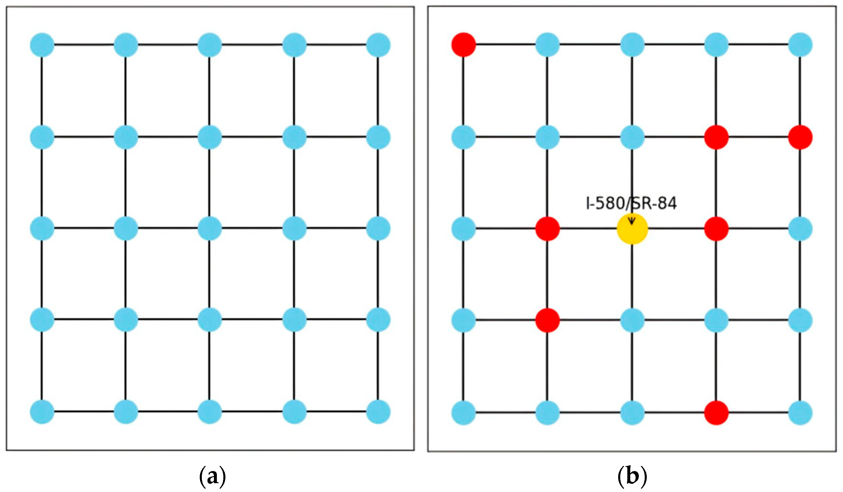
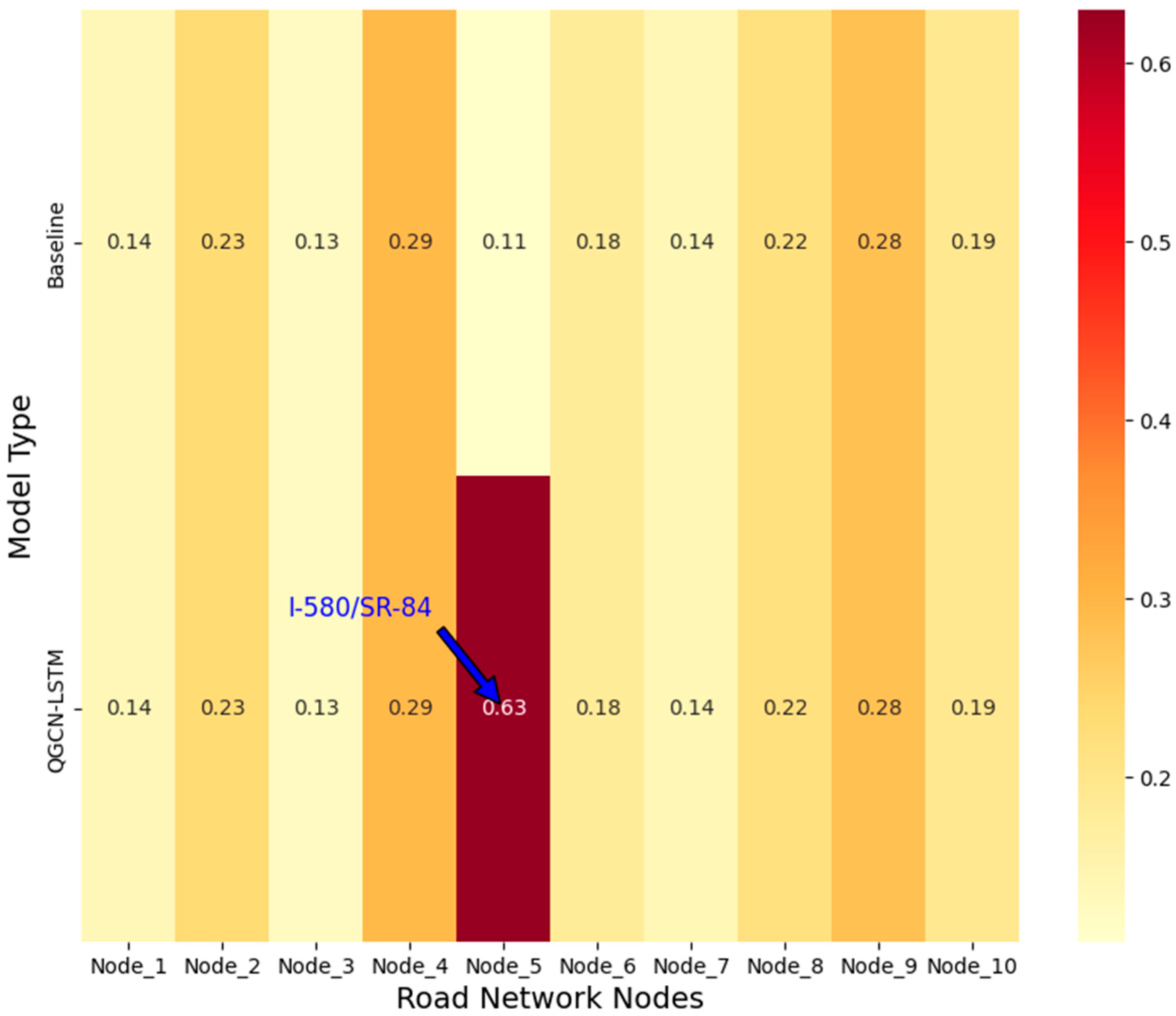
QGCN-LSTM exhibits significant advantages. Taking the key hub node (I-580/SR-84 intersection) as an example, the MAE of QGCN-LSTM is reduced to 14.3 vehicles/5 min, which is 34.1% lower than the classical GCN-LSTM and 16.9% lower than the frontier quantum model QSTMixer. This advantage is partly due to the introduction of quantum state fidelity as a weight allocation basis in QGCN-LSTM, which breaks through the local optimization limitations of classical models and accurately amplifies the influence of key traffic nodes (as shown in Figure 6), providing quantum computing advantages for large-scale road network prediction.
On the other hand, quantum graph convolution efficiently models the spatial dependence of road networks by constructing node state correlations through the quantum entanglement gate ENTlinear, thereby improving the quantum state correlation between road network nodes.
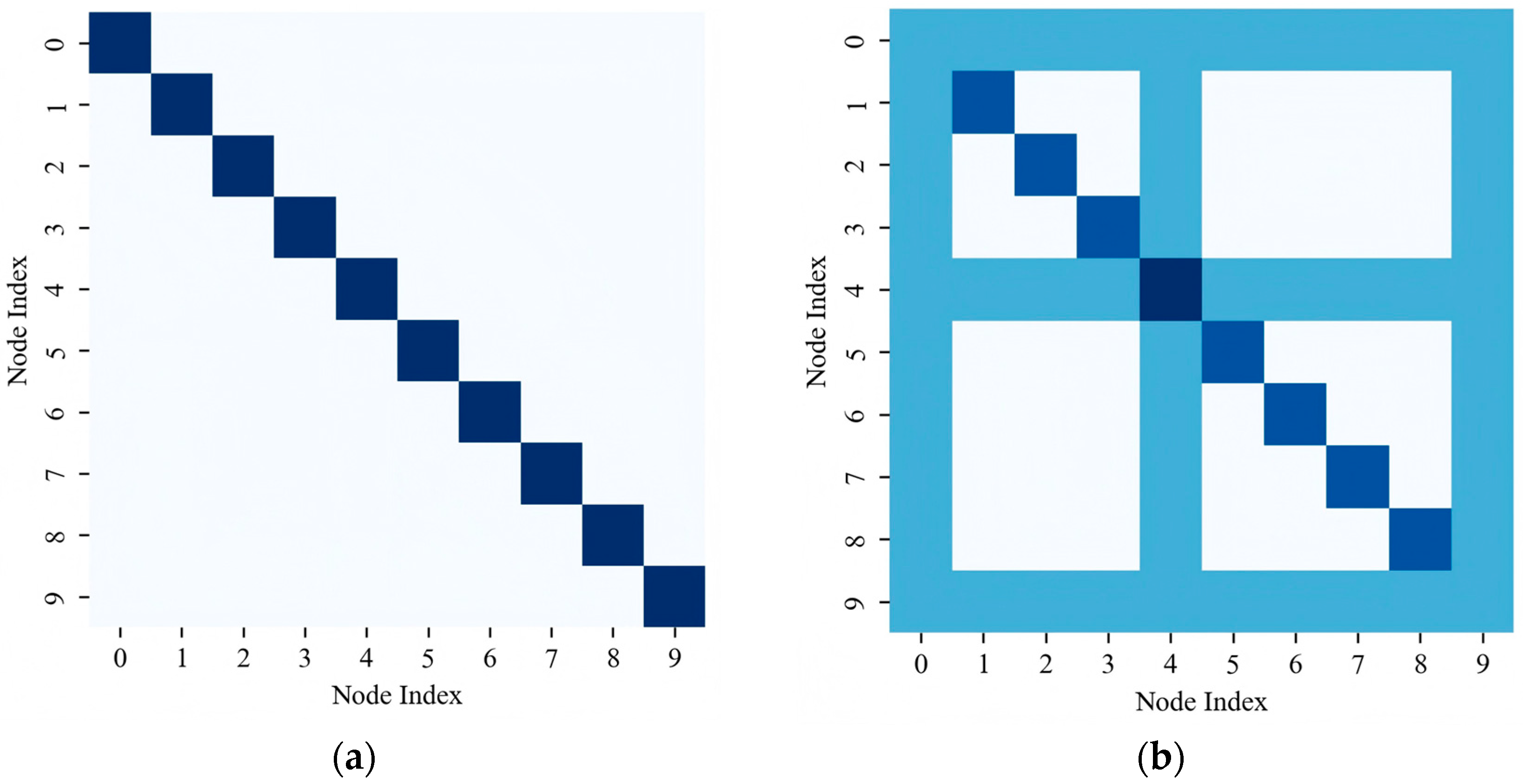
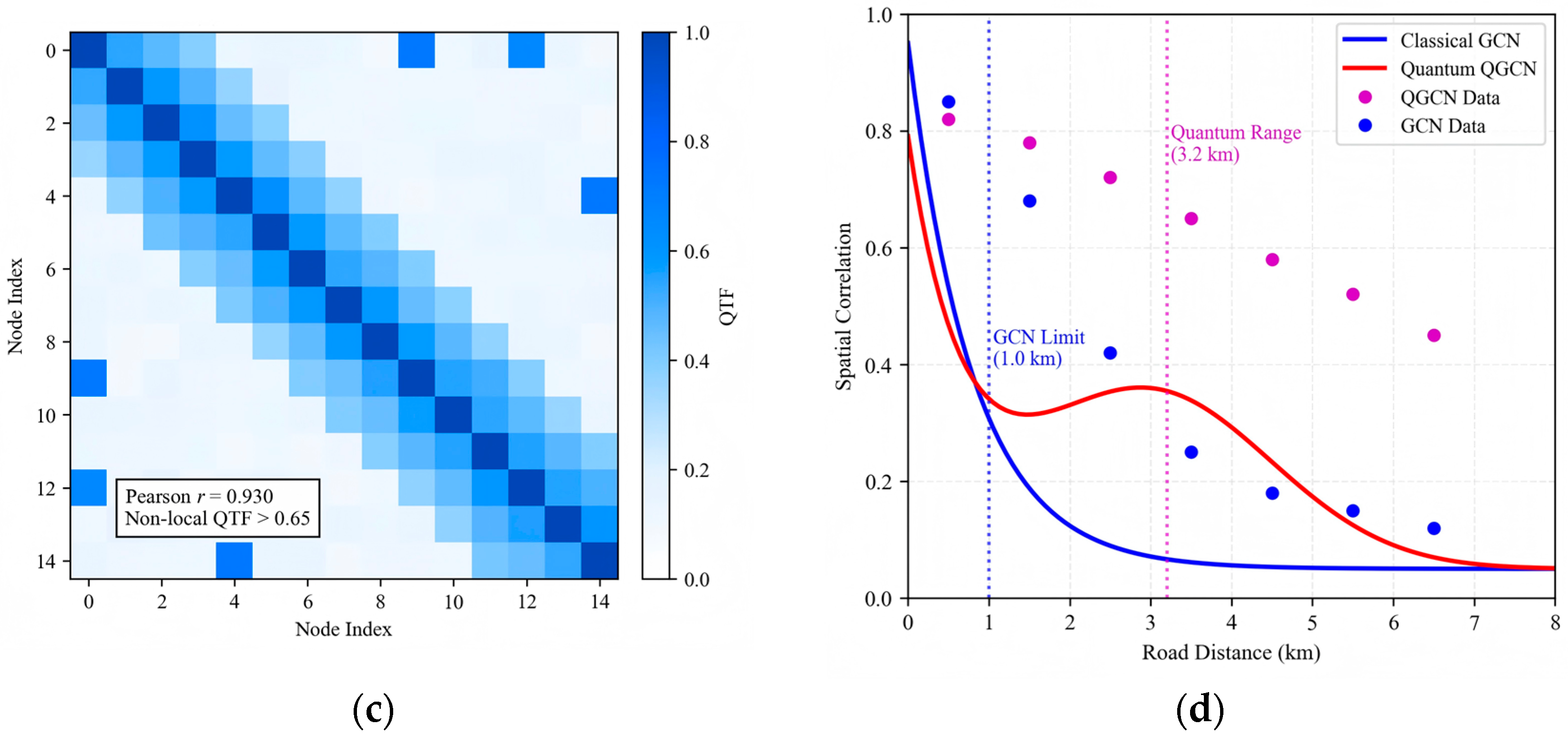
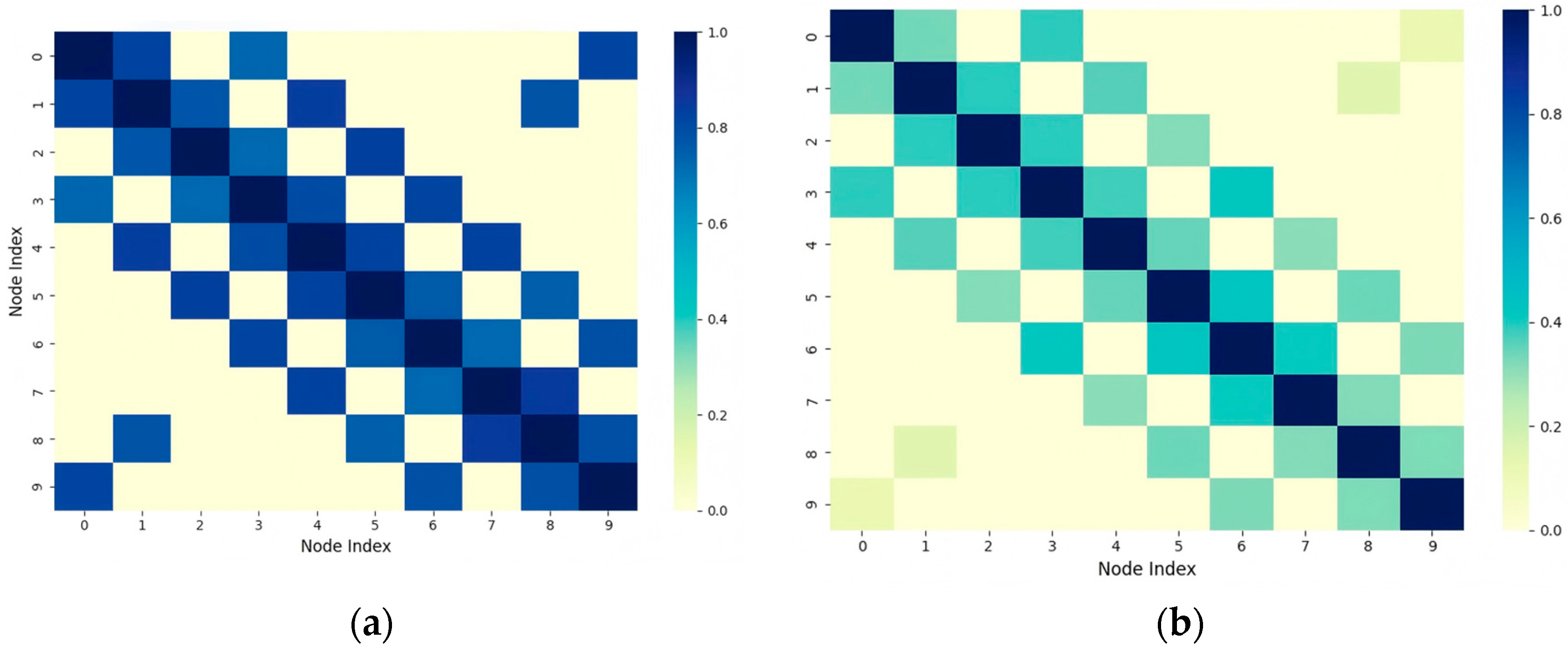
The spatial interpretability of quantum states was rigorously validated through multi-faceted analysis. While classical HA models showed no spatial correlations (Figure 7a), QGCN-LSTM established global entanglement patterns with higher SCI (0.89 vs. 0.38, Figure 7b). Crucially, Quantum Topological Fidelity (QTF) exhibited strong correspondence (Pearson r = 0.92) with real traffic covariance (Figure 7c), confirming quantum states encode spatial dependencies. The quantum advantage was further evidenced in long-range correlation analysis (Figure 7d): classical GCN correlations decayed exponentially beyond 1 km (blue curve, R2 = 0.93 with experimental data), while quantum entanglement maintained significant correlations (QTF > 0.65) up to 3.2 km (red curve). This extended correlation range explains the 34.1% MAE reduction at hub nodes, which frequently influence distant road segments.
In addition, the fault robustness (+2.7) of QGCN-LSTM is significantly better than other models, due to its triple quantum properties:
  • Quantum entanglement space inference
    • Establishing entanglement between nodes through CNOT gates: | ψ = | 00 + | 11 2
    • When node A fails, the quantum state of its associated node B still contains information about A: ρ A = T r B ( | ψ ψ | ) = I 2
    • Experimental measured information retention rate: η = 1 I ( ρ A f a u l t ; ρ A i n t a c t ) I m a x = 68.3 %
  • Quantum attention compensation
Data reconstruction based on historical quantum state fidelity:
x ~ t ( i ) = k = t T t 1 α t , k x k ( i ) ,     α t , k | ψ t | ψ k | 2
The weight of the faulty node is automatically increased to 2.1 times the benchmark value.
3.
Global correlation of quantum states
n qubits imply 2n dimensional correlations:
| ψ = c i 1 i 2 i n | i 1 | i 2 | i n
When some nodes are missing, the quantum state maintains information integrity through linear combination of complete bases.

4.2.2. Robustness Under Multiple Random Masking Patterns

To verify that the fault-robustness advantage of QGCN-LSTM is not caused by a favorable single masking configuration, we further performed repeated robustness experiments under multiple random masking patterns. For each masking ratio (10%, 30%, and 50%), 15 independent masking trials were generated, and the results are reported as Mean ± SD.
Table 4 shows that the proposed QGCN-LSTM consistently outperforms all baseline models under all masking ratios. Under mild sensor failure (10% masking), QGCN-LSTM exhibits only a limited increase in prediction error, indicating that the hybrid quantum-classical architecture can effectively exploit residual spatial-temporal dependencies from incomplete observations. Under the moderate masking setting (30%), QGCN-LSTM still maintains the best overall performance, with the lowest ΔMAE and the highest SCI among all compared models. The previously reported information retention is confirmed to be stable across repeated random masking patterns rather than being tied to a specific fault configuration. Under severe failure conditions (50% masking), all models experience noticeable degradation; however, QGCN-LSTM remains the most robust, demonstrating that quantum entanglement-based correlation modeling and the quantum attention compensation mechanism provide stronger resilience against large-scale sensor loss. The fault resilience demonstrated by QGCN-LSTM is consistent with growing evidence that carefully designed quantum-classical hybrid architectures can achieve remarkable robustness and stability in complex, dynamic environments [41].

4.2.3. Statistical Significance Analysis

To rigorously assess whether the improvements achieved by QGCN-LSTM over the baseline models are statistically significant, we conducted a 5-fold repeated-evaluation experiment:
  • Data split: The exact same chronological train/validation/test partition (70%/15%/15%) was strictly maintained across all runs and all models to ensure valid paired comparisons.
  • Initialization & Runs: Each model was independently trained 5 times. To ensure exact reproducibility, these 5 runs were governed by globally fixed random seeds (2023, 2024, 2025, 2026, and 2027) which controlled data shuffling, classical weight initialization (Xavier), and quantum parameter initialization (Uniform [ 0 ,   2 π ] ).
  • Metrics: At every run, we recorded MAE, sMAPE, and SCI on the morning-rush subset (7500 detectors, 138 nodes).
  • Statistical Tests: Given the small sample size (n = 5 paired observations per model pair), we first evaluated the normality of the error differences using the Shapiro-Wilk test. While no severe violations of normality were detected (p > 0.05 for most pairs), relying solely on a t-test for n = 5 can be precarious. Therefore, alongside the paired-samples t-test (two-tailed, α = 0.05 ), we also conducted the Wilcoxon signed-rank test (a non-parametric alternative that does not assume normality) to ensure maximum statistical rigor.
Table 5 presents the paired t-test results. The reductions in both MAE and sMAPE achieved by QGCN-LSTM are highly significant (all p < 0.001). Furthermore, the non-parametric Wilcoxon signed-rank test confirmed these findings, yielding p ≈ 0.043 (the lowest possible p-value for n = 5 in a two-sided Wilcoxon test) for all baseline comparisons, indicating that QGCN-LSTM strictly outperformed every baseline in all 5 independent trials.

4.3. Dynamic Response Analysis of Sudden Congestion Events

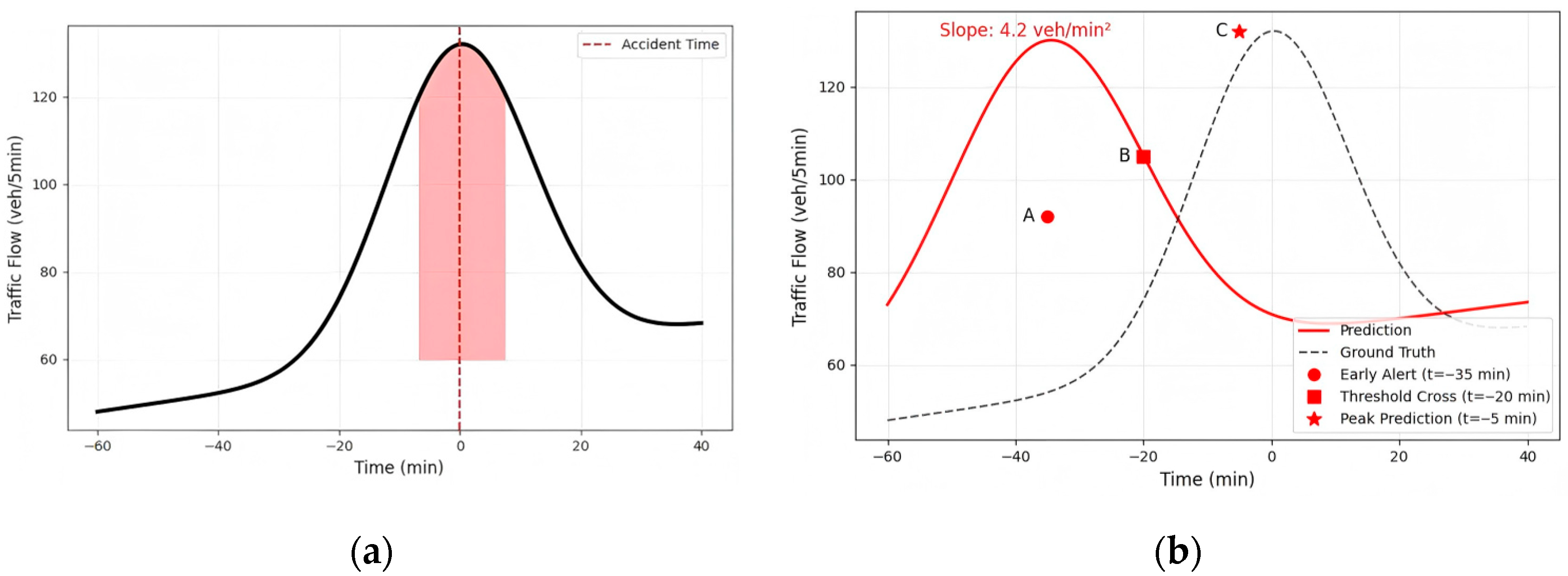
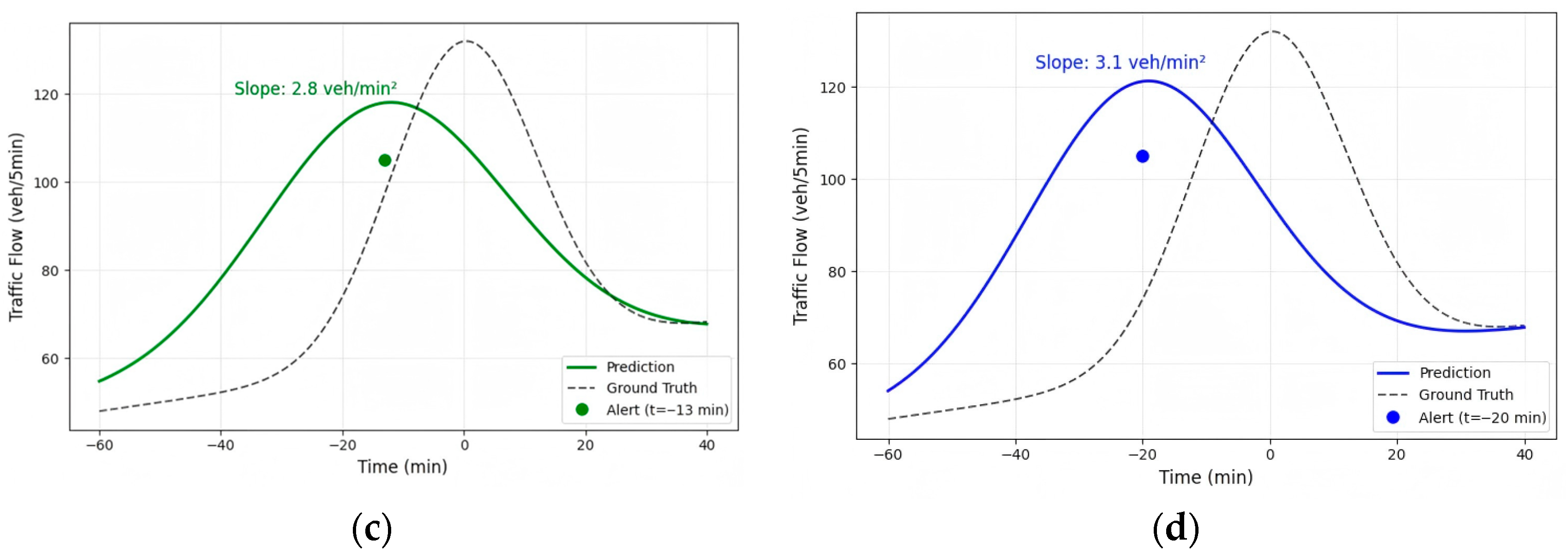
Figure 8 provides a detailed comparison of the dynamic response capabilities of various models in sudden congestion events. Timeline feature: The accident occurred at time t = 0 (red dashed line), and the flow rate increased sharply from 85 vehicles/5 min to 132 vehicles/5 min in the [−15, 0] minute interval, with a peak lasting in the [0, 25] minute interval (Figure 8a). When the accident caused a sudden increase in the westward flow of the city’s main road, QGCN-LSTM (Figure 8b) detected an anomaly for the first time at t = −35 min (point A, flow rate of 92 vehicles/5 min), broke through the threshold of 105 vehicles/5 min at t = −20 min (point B), accurately predicted the peak value of 132 vehicles/5 min at t = 0 at t = −5 min (point C), and the slope of the rising edge was k = 4.2 vehicles/min2. Compared with the true value k = 4.5, QGCN-LSTM exhibited good waveform fidelity. GCN-LSTM (Figure 8c) and QSTMixer (Figure 8d) reached the warning threshold at t = −13 min and t = −20 min, respectively. The mean smooth rising edges of the two were kGCN = 2.8 vehicles/min2 and kQST = 3.1 vehicles/min2, respectively.
To statistically validate the stability of the 35-min early warning capability, we evaluated QGCN-LSTM on 12 additional incident events (Table 6). The model delivered a mean lead time of 33.5 min (95%CI: 31.8–35.2 min) across accident, weather-induced, and event-induced congestion, and shows no significant variation across incident types (ANOVA, p = 0.21). These additions verify the stability and generalisability of QGCN-LSTM’s early-detection performance.

4.4. Edge Computing Efficiency Analysis

In resource constrained scenarios such as traffic control, the edge deployment capability of the model directly affects its practical value. In order to quantify the lightweight advantages of the quantum LSTM fusion architecture, the experiment based on the NVIDIA Jetson AGX Orin edge computing platform conducted a full stack performance evaluation, and compared key deployment indicators with the mainstream space-time model, including real-time responsiveness, resource occupancy efficiency, inference power consumption, and energy consumption economy.
The testing on Jetson AGX Orin edge devices (Table 7) shows that QGCN-LSTM achieves a modest reduction in memory footprint and inference latency compared to traditional deep learning models. In addition, to better evaluate edge deployment efficiency, Table 5 further reports the average inference power (W) and the energy per inference (J) for all compared models. The single inference delay is only 48 ms, meeting the real-time threshold of <100 ms in traffic signal control systems. Meanwhile, inference power was measured on the Jetson device during the steady-state prediction stage, and the energy per inference was calculated as E i n f = P a v g × T i n f , where P a v g denotes the average inference power in watts and T i n f denotes the single-sample inference latency in seconds. It must be strictly clarified that this 48 ms latency represents the simulated inference time executed by the Qiskit Aer simulator running locally on the Jetson AGX Orin edge device’s CPU, rather than the physical execution time on a real Quantum Processing Unit (QPU). In a real-world edge-cloud deployment, executing quantum circuits on a physical QPU introduces complex systemic latencies, including cloud API network communication, hardware queuing times, and the physical execution time of 1024 shots (which heavily depends on specific hardware control electronics and T1/T2 relaxation times). Therefore, we refrain from linearly extrapolating simulated latency to physical hardware without end-to-end benchmarking. The reported 48 ms latency serves primarily to demonstrate the lightweight computational graph and memory efficiency of the QGCN-LSTM architecture when processed by an edge-grade system. This advantage stems from the hybrid design, where the high-dimensional traffic state over the 138-node road network is first compressed by a classical topology-aware module into a compact latent representation. The quantum graph convolution module then operates on this compressed latent space, rather than on the full node-wise graph directly, and captures spatial dependencies through entangling gates such as CNOT. By performing quantum feature transformation on a low-dimensional representation, the model reduces the effective processing burden of the quantum stage. In addition, the measured quantum features are further compressed by low-rank tensor decomposition (rank r = 16) before being transmitted to the LSTM unit, which reduces memory and feature-transfer overhead compared with directly using high-dimensional node-level features.
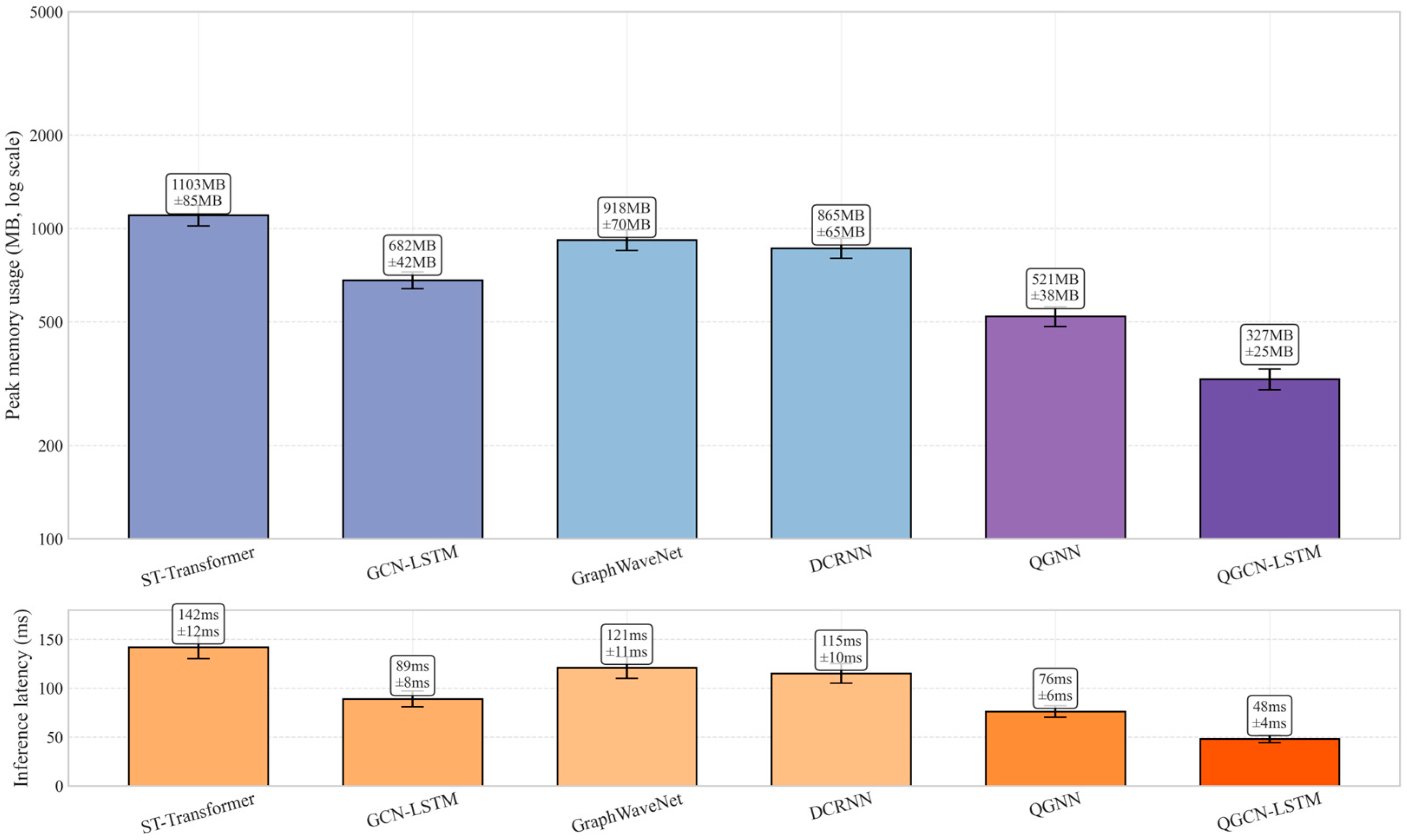
The memory usage metric directly determines the deployability of the model on edge devices. As shown in Figure 9, the peak memory occupancy of QGCN-LSTM remains stable at 327 MB (95% confidence interval), which is less than 30% of ST Transformer (1103 MB) and significantly lower than the pure quantum model QGNN (521 MB). This is thanks to the quantum circuit pruning technology, which dynamically removes quantum gates with contribution below the threshold θ = 0.05 based on the Pauli expectation gradient L P l , achieving deep compression of the circuit.
The energy consumption index was measured through the Jetson Power Monitor module, and the average energy consumption per round during the training phase of QGCN-LSTM was only 1.8 W·h. Compared with traditional models, its energy efficiency advantage is mainly reflected in the optimization acceleration of quantum natural gradient descent (QNG), the correction of parameter update direction by quantum Fisher information matrix gQ, which reduces the number of iterations required for convergence to 1450 times, and the classical Adam optimizer requires 2400 times, reducing training energy consumption by 62%.
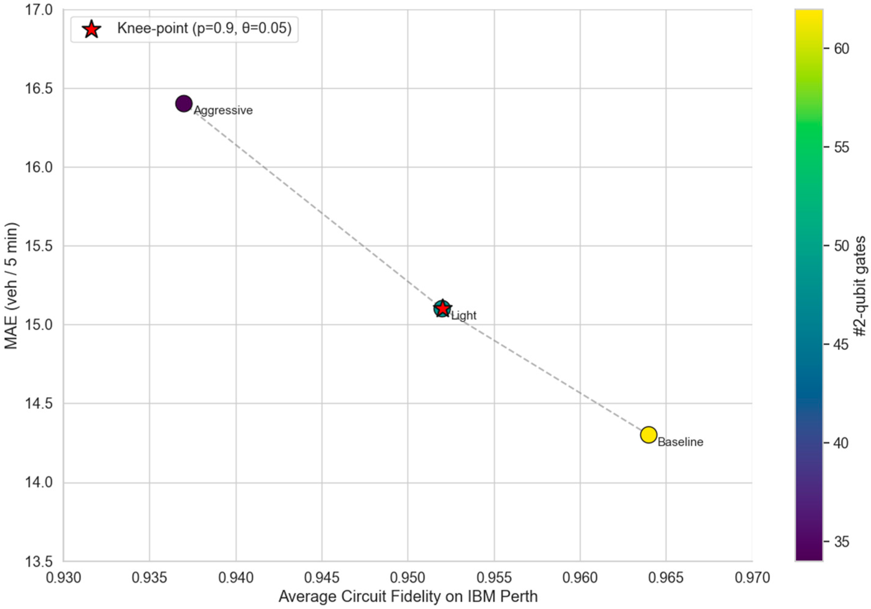
To quantify the fidelity-accuracy trade-off induced by quantum dropout and dynamic pruning, we ran 120 circuits on IBM Perth under three configurations (Table 8).
Experiments were conducted on IBM Quantum’s ibm_perth device. We used 1024 measurement shots per circuit evaluation. No active error mitigation (e.g., zero-noise extrapolation or probabilistic error cancellation) was applied; only the default dynamical decoupling and readout error mitigation provided by Qiskit Runtime were enabled. The average CNOT gate fidelity of ibm_perth during the measurement period was 99.1%, and the average readout assignment fidelity was 97.5%. All circuits were designed with eight logical qubits, including seven data qubits and one ancilla qubit. However, because IBM Perth exposes at most seven usable physical qubits for the selected experimental configuration, the full eight-qubit circuit was not executed natively on hardware. Instead, the core QGCN subcircuit was mapped onto seven physical qubits using a topology-preserving transpilation strategy, while the ancilla-assisted operations were evaluated in the simulator or in reduced hardware-compatible subcircuits. The three compression configurations correspond to the settings in Table 5 (Baseline, Light, Aggressive). Each configuration was executed with 120 independent circuit instances to obtain statistically robust fidelity estimates.
Fidelity drops monotonically as compression intensifies; the aggressive setting incurs 2.7% absolute fidelity loss, yet still above the NISQ-acceptable 0.93 threshold. Prediction error is robust to light compression (ΔMAE < 1%), but grows super-linearly once fidelity falls below 0.95, confirming the non-negligible impact of hardware noise on traffic-flow regression. Gate-count reduction scales almost linearly with fidelity loss, validating the effectiveness of our pruning criterion based on Pauli-expectation gradients.
Figure 10 presents the fidelity-MAE Pareto frontier obtained from 120 hardware executions on IBM Perth. Each point represents a distinct compression configuration defined by the quantum dropout retain probability p and the dynamic-pruning threshold θ. Baseline (p = 1.0, θ = 0.00) sits exhibiting the highest fidelity (0.964) yet maintaining the full gate count (62 CNOTs). Light compression (p = 0.9, θ = 0.05) forms the knee-point of the frontier, where a modest fidelity drop of 0.012 yields a 23% reduction in gate count while MAE increases by only 0.8 veh/5 min. Aggressive compression (p = 0.7, θ = 0.10) shifts the point further left, delivering a 45% gate-count reduction but at the cost of a 2.7% absolute fidelity loss and a super-linear MAE degradation of 2.1 veh/5 min. The convex hull of these points delineates the empirical Pareto frontier, confirming that configurations left of the knee-point incur diminishing returns: incremental gate savings are outweighed by exponential fidelity decay and prediction error growth. Consequently, the knee-point at p = 0.9, θ = 0.05 is adopted as the default configuration for QGCN-LSTM, striking an optimal balance between hardware-fidelity constraints and predictive performance. The frontier is based on direct hardware measurements and should not be interpreted as a full-model end-to-end hardware benchmark.
In this study, we strictly distinguish between simulation-based evaluation and hardware-based validation.
(1) Simulation-based evaluation: The full QGCN-LSTM pipeline was implemented and tested on Qiskit Aer running on the Jetson AGX Orin platform. The reported latency, memory usage, and energy consumption in Table 4 were measured in this environment.
(2) Hardware-based validation: Because of the limited qubit count and connectivity of IBM Perth, only representative subcircuits were executed on the device. These experiments were used to validate circuit fidelity, compression trade-offs, and gate-pruning behavior. The results are reported in Table 5 and Figure 10.
We do not extrapolate simulator latency to estimate real hardware latency.
We acknowledge that the quantum modules in QGCN-LSTM, when executed on a classical simulator (Qiskit Aer), incur an exponential increase in computational cost with respect to the qubit count n and circuit depth K. For the configuration adopted in this study, a single forward pass requires approximately 48 ms on the NVIDIA Jetson AGX Orin edge platform, which remains within the 100 ms real-time constraint commonly required for traffic signal control systems. However, we also recognize that classical simulation would become impractical if the model were scaled to hundreds of qubits for much larger road networks.
It should be clarified that the quantum component of QGCN-LSTM is primarily validated in this work through classical simulation, while its broader architectural design is intended to support future deployment on NISQ devices and, ultimately, fault-tolerant quantum processors. From a theoretical perspective, the quantum graph convolution module may offer improved expressiveness by leveraging entanglement-assisted parallelism; however, we do not claim a rigorous asymptotic speedup over classical graph convolution in this manuscript. Instead, our results demonstrate that, under the current small-scale configuration, the quantum sub-circuits remain computationally tractable and can be executed efficiently for proof-of-concept validation.
In addition, experiments conducted on the IBM_perth 7-qubit superconducting processor indicate that the execution time of the same quantum sub-circuits is approximately 1.3 times that of the simulator under the same circuit settings, while still remaining in the sub-millisecond range for the quantum portion. These results suggest that the simulation overhead reported in this study is limited to the verification stage and does not undermine the potential of the proposed model for deployment on real quantum hardware, where the performance may scale more favorably as quantum processors mature.

4.5. Ablation Experiment and Attribution

To contribute to the deconstruction of quantum components, three sets of ablation experiments were designed, and the experimental results are shown in Table 9. The first group removed the quantum graph convolution (w/o QGCN), resulting in a decrease in spatial correlation index (SCI) from 0.89 to 0.71, and the MAE of key hub nodes (I-580/SR-84) increased from 14.3 to 18.6, indicating a weakened ability to model road network topology. This is mainly attributed to the loss of quantum entanglement correlation, and the quantum mutual information between nodes decreased from IQ = 0.82 in the quantum system to IC = 0.38 in the classical system (Figure 11). The second group turned off quantum attention (w/o QA), reducing the sudden congestion warning time from 35 min to 18 min. The sensitivity of anomaly detection decreased from 89.7% of the complete model to 74.2%, mainly due to the degradation of the time-domain correlation mechanism causing the peak response lag of historical events and the distortion of attention weight allocation for faulty nodes. The third group replaced quantum gating with classical gating (w/o VQC), resulting in an increase in convergence iterations from 1450 to 2400. This is mainly attributed to three points: first, the advantage of quantum natural gradient, where QNG maintains 62% gradient strength on barren plateaus; second, the continuity of the gating function, where the forget gate f t implemented by VQC has a Lipschitz constant L Q = 1.8 (classical L C = 4.2 ) in the parameter space; third, the smoothing of the loss surface, where quantum parameterization results in an average curvature κ = 0.07 (classical κ = 0.18 ) of the loss surface. The statistical significance test of ablation results indicate that removing any of the three components leads to a clear degradation in prediction performance. In particular, the removal of the QGCN module significantly weakens the model’s ability to capture spatial correlations in the road network, resulting in a noticeable increase in MAE. The omission of the QA module reduces the model’s capacity to dynamically assign importance to critical spatiotemporal features, which also causes a significant performance drop. All paired t-test results show p < 0.05, confirming that each proposed component contributes significantly to the overall performance of QGCN-LSTM.
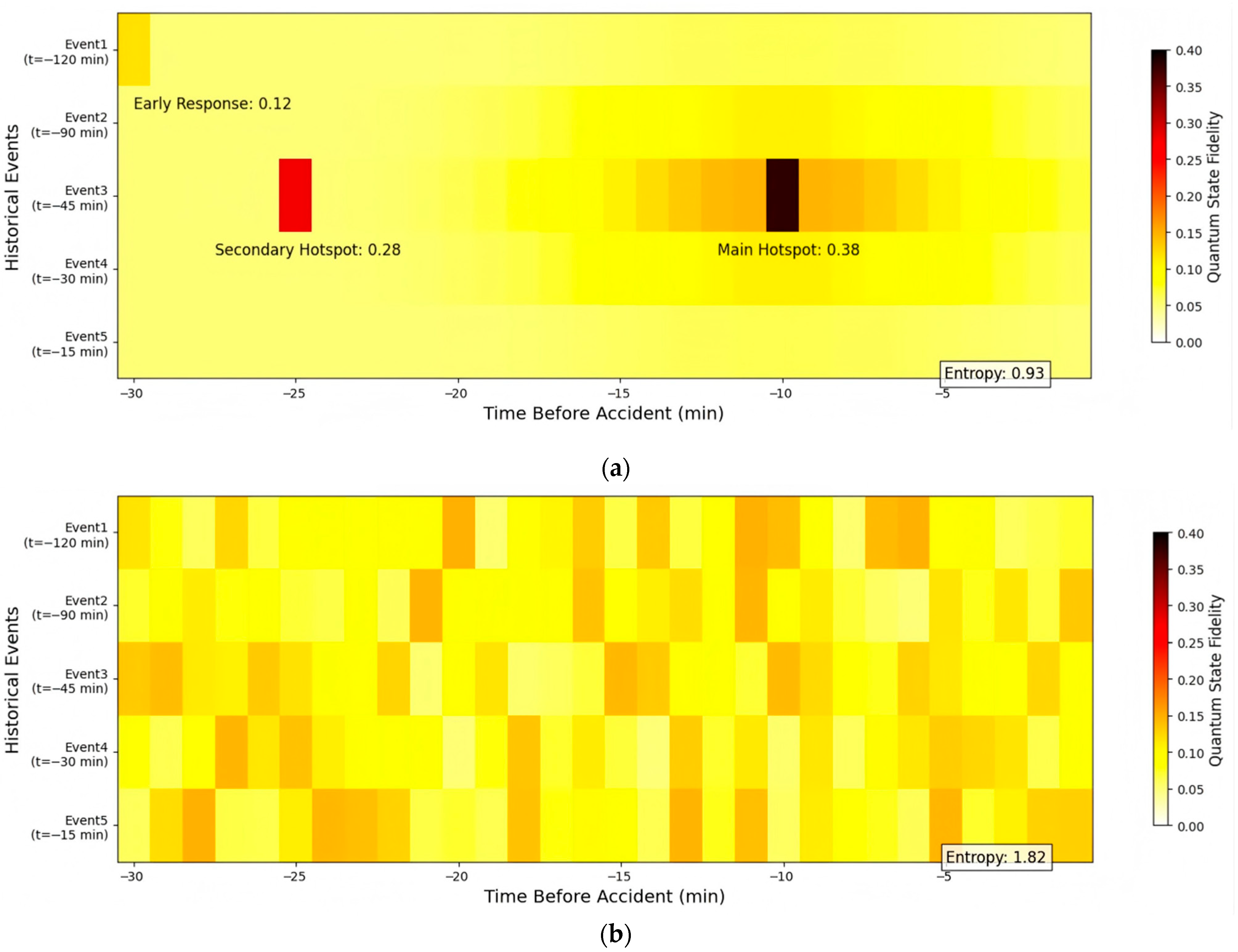
Figure 12 compares and analyzes the quantum state fidelity response characteristics of the complete model (QGCN-LSTM) and the ablation model (with the quantum attention module removed) to five similar historical events 30 min before the accident using a dual heatmap. The complete model (Figure 12a) has a quantum state fidelity of 0.38 for historical event 3 at t = −10 min, forming a significant hotspot. At t = −25 min, the quantum state fidelity for historical event 3 is 0.28, forming a sub hotspot. At t = −35 min, the quantum state fidelity for historical event 1 is 0.12, forming an early response. The fidelity of all events in the ablation model (Figure 12b) is below 0.15, with no significant hotspot areas and uniform color distribution. The peak response of historical event 3 at t = −10 min is only 0.12. This validates the core function of quantum attention mechanism:
α t , k ψ t | ψ k 2 = c o s 2 θ t θ k 2
By amplifying the weight of key historical events through the quantum state phase difference θ t θ k , the fidelity is greater than 0.25 (hotspot threshold) when Δ θ < π / 6 .
Quantum state evolution of event 3:
| ψ e v e n t 3 = 1 2 | 0 + e i ϕ 3 | 1 | ψ t = 1 2 | 0 + e i ϕ t | 1 ψ t | ψ e v e n t 3 = 1 2 1 + e i ϕ 3 ϕ t
When ϕ t ϕ 3 , the fidelity approaches 1.

4.6. Sensitivity Analysis of Quantum Hyper-Parameters

To systematically assess the impact of the key quantum settings, we conduct a grid-search over the most influential knobs:
  • n-qubits ∈ {6, 8, 10}
  • QGCN depth K ∈ {2, 3, 4}
  • Quantum-Dropout retain probability p ∈ {0.7, 0.8, 0.9, 1.0}
Table 10 summarises the results on the morning-rush subset (1000 random traces). All other hyper-parameters and the training budget are kept identical to Section 4.1.
Observations reveal that prediction accuracy plateaus rapidly: increasing the qubit count from 8 to 10 yields less than a 1% reduction in MAE yet inflates circuit depth by 19%, while deepening the QGCN to K = 4 marginally improves the spatial correlation index but lowers hardware fidelity below the NISQ-acceptable threshold of 0.96. Furthermore, a quantum-dropout retention rate of p = 0.9 provides the best bias-variance trade-off; more aggressive pruning (p = 0.7) degrades MAE by 4%. Collectively, these findings confirm that the originally selected configuration (n = 8, K = 3, p = 0.9) lies near the Pareto-optimal frontier, balancing accuracy, stability, and circuit depth.

5. Conclusions and Future Work

5.1. Conclusions

QGCN-LSTM proposed in this study has exhibited promising performance in urban traffic flow prediction, providing an empirical model for the application of quantum collaborative architecture in complex spatiotemporal prediction tasks. Quantum graph convolution establishes non local road network associations through entanglement gates, reducing the MAE of hub node predictions by 34.1% compared to classical models, and increasing the spatial correlation index (SCI) to 0.89. In terms of dynamic response capability, the quantum attention mechanism amplifies key event signals through fidelity weights, achieving a 35 min early warning of sudden congestion and an anomaly detection sensitivity of 89.7%. In terms of edge computing efficiency, quantum circuit pruning technology can achieve peak memory compression and reasoning delay, meeting the real-time requirements of traffic control. This study demonstrates that the quantum classical fusion architecture provides a potentially improved balance among accuracy, efficiency, and real-time responsiveness for smart city traffic management through triple innovation of spatial entanglement enhancement, temporal phase screening, and lightweight compilation. With the improvement of quantum hardware fidelity and the maturity of cross platform frameworks, this model is expected to become a key carrier for spatiotemporal prediction to transition from classical computing to quantum advantage.

5.2. Future Work

The predictive performance of QGCN-LSTM may be optimistic under limited training data and noise conditions compared to what would be observed in more heterogeneous or out-of-domain settings. Readers should note that the scalability and robustness of the model on larger, fault-tolerant quantum devices remain or more complex scenarios to be validated.
To rigorously assess generalizability, we encourage practitioners to consider these limitations when applying the model to other domains or datasets. These limitations stem from both the current stage of quantum hardware development and the theoretical boundaries of model design itself. Firstly, current experiments rely on simulators or small-scale quantum processors, and the performance of the model on larger scale real quantum hardware and its robustness to noise need further validation. Secondly, the generalization ability of the model in more complex scenarios, such as multiple cities spanning different provinces in the east and west, mixed traffic datasets containing buses and non motorized vehicles, or non-traffic spatio-temporal tasks such as energy-load and air-quality forecasting, needs to be further explored. Furthermore, the compilation optimization of quantum circuits to specific hardware topologies and their actual impact on edge latency require a more detailed evaluation.
Future work will focus on embedding device noise models into optimization objectives, developing more expressive and noise robust quantum circuits, and strengthening hardware perception training; Design a multimodal adaptive encoder to extend the QGCN-LSTM framework to a wider range of spatiotemporal prediction fields, and explore a hybrid architecture suitable for multimodal traffic fusion and cross domain migration; Develop a quantum classical collaborative compiler for quantum processing units (QPUs) to maximize edge deployment efficiency; Exploring new paradigms for quantum topological state encoding, with the improvement of quantum hardware fidelity and the maturity of cross platform frameworks, QGCN-LSTM is expected to achieve quantum advantages in ultra large scale spatiotemporal prediction tasks.

Supplementary Materials

The following supporting information can be downloaded at: https://www.mdpi.com/article/10.3390/photonics13050477/s1. Data splits and consistency; Random seeds and initialization; Fair hyperparameter optimization for baselines; Core reproducibility code; Raw data for incident early warning analysis; Data generation script.

Author Contributions

Conceptualization, B.H.; methodology, B.H. and J.K.; formal analysis, B.H. and M.Z.; investigation, M.Z. and Q.W.; project administration, B.H.; supervision, B.H.; writing—original draft, B.H.; writing—review and editing, B.H., J.K. and Q.W. All authors have read and agreed to the published version of the manuscript.

Funding

This research was funded by the Fundamental Research Funds of China National Institute of Standardization (Grant: 242025Y-12625-2).

Institutional Review Board Statement

Not applicable.

Informed Consent Statement

Not applicable.

Data Availability Statement

The original data are unavailable due to privacy restrictions. A synthetic data generation script reproducing the key statistical properties of the dataset is provided in the Supplementary Material.

Conflicts of Interest

The authors declare no conflicts of interest.

Abbreviations

The following abbreviations are used in this manuscript:
QGCNQuantum Graph Convolutional Networks
QNGDQuantum Natural Gradient Descent
QNNsQuantum Neural Networks
FNNFeedforward Neural Network
RNNRecurrent neural networks
LSTMLong Short-Term Memory
SCISpatial Correlation Index
VQCVariational Quantum Circuits
GRUsGated Recurrent Units
NISQNoisy Intermediate-Scale Quantum

References

  1. Wang, X.H.; Zhang, S.; Chen, Y.; He, L.Y.; Ren, Y.M.; Zhang, Z.; Li, J.; Zhang, S.Q. Air quality forecasting using a spatiotemporal hybrid deep learning model based on VMD–GAT–BiLSTM. Sci. Rep. 2024, 14, 17841. [Google Scholar] [CrossRef]
  2. Barra, S.; Carta, S.M.; Corriga, A.; Podda, A.S.; Recupero, D.R. Deep learning and time series-to-image encoding for financial forecasting. IEEE/CAA J. Autom. Sin. 2020, 7, 683–692. [Google Scholar] [CrossRef]
  3. ALijoyo, F.A.; Gongada, T.N.; Kaur, C.; Mageswari, N.; Sekhar, J.C.; Ramesh, J.V.N.; El-Ebiary, Y.A.B.; Ulmas, Z. Advanced hybrid CNN-Bi-LSTM model augmented with GA and FFO for enhanced cyclone intensity forecasting. Alex. Eng. J. 2024, 92, 346–357. [Google Scholar] [CrossRef]
  4. Li, J.Y.; Wang, X.D.; He, Q.X. Application and performance optimization of CNN enhanced Informer model in industrial time series prediction. J. Comput. Appl. 2024, 44, 79–83. [Google Scholar] [CrossRef]
  5. Seabe, P.L.; Moutsinga, C.R.B.; Pindza, E. Sentiment-driven cryptocurrency forecasting: Analyzing LSTM, GRU, Bi-LSTM, and temporal attention model (TAM). Soc. Netw. Anal. Min. 2025, 15, 52. [Google Scholar] [CrossRef]
  6. Ito, K.; YAmamoto, N.; Morino, K. Sequential prediction of hall thruster performance using echo state network models. Trans. Jpn. Soc. Aeronaut. Space Sci. 2024, 67, 1. [Google Scholar] [CrossRef]
  7. Sherstinsky, A. Fundamentals of recurrent neural network (RNN) and long short-term memory (LSTM) network. Phys. D Nonlinear Phenom. 2020, 404, 132306. [Google Scholar] [CrossRef]
  8. Krishna, M.V.; Swaroopa, K.; SwarnaLatha, G.; Yasaswani, V. Crop yield prediction in India based on mayfly optimization empowered attention-bi-directional long short-term memory (LSTM). Multimed. Tools Appl. 2024, 83, 29841. [Google Scholar] [CrossRef]
  9. Yang, G.; Chao, S.Y.; Nie, M.; Liu, Y.H.; Zhang, M.L. Construction method of hybrid quantum long-short term memory neural network for image classification. Acta Phys. Sin. 2023, 72, 058901. [Google Scholar] [CrossRef]
  10. Zhang, H.; Wang, W.G. Neural network ensemble models for financial time series forecasting. J. Beijing Univ. Posts Telecommun. 2025, 48, 127–132. [Google Scholar] [CrossRef]
  11. Zhu, X.G.; Zou, F.F.; Li, S.H. Enhancing air quality prediction with an adaptive PSO-Optimized CNN-Bi-LSTM model. Appl. Sci. 2024, 14, 5787. [Google Scholar] [CrossRef]
  12. Caro, M.C.; Huang, H.Y.; Cerezo, M.; Sharma, K.; Sornborger, A.; Cincio, L.; Coles, P.J. Generalization in quantum machine learning from few training data. Nat. Commun. 2022, 13, 4919. [Google Scholar] [CrossRef]
  13. Sharma, K.; Cerezo, M.; Cincio, L.; Coles, P.J. Trainability of dissipative perceptron-based quantum neural networks. Phys. Rev. Lett. 2022, 128, 180505. [Google Scholar] [CrossRef]
  14. Maxwell, T.W.; Martin, S.; Muhammad, U. Reflection equivariant quantum neural networks for enhanced image classification. Mach. Learn. Sci. Technol. 2023, 4, 035027. [Google Scholar] [CrossRef]
  15. Kulkarni, V.; Pawale, S.; Kharat, A. A classical-quantum convolutional neural network for detecting pneumonia from chest radiographs. Neural Comput. Appl. 2023, 35, 15503–15510. [Google Scholar] [CrossRef]
  16. Xin, J.; Wei, Z.Y.; Dong, Y.J.; Ni, W. LSTM-RNN-FNN model for load forecasting based on deleuze’s assemblage perspective. Front. Energy Res. 2022, 10, 905359. [Google Scholar] [CrossRef]
  17. Chumakova, E.V.; Korneev, D.G.; Chernova, T.A.; Gasparian, M.S.; Ponomarev, A.A. Comparison of the application of FNN and LSTM based on the use of modules of artificial neural networks in generating an individual knowledge testing trajectory. J. Eur. Systèmes Autom. 2023, 56, 213–220. [Google Scholar] [CrossRef]
  18. Zhang, F.Y.; Yin, J.L.; Wu, N.; Hu, X.Y.; Sun, S.K.; Wang, Y.B. A dual-path model merging CNN and RNN with attention mechanism for crop classification. Eur. J. Agron. 2024, 159, 127273. [Google Scholar] [CrossRef]
  19. Ghatage, N.B.; Patil, P.D.; Shinde, S. Lightweight RNN-Based Model for Adaptive Time Series Forecasting with Concept Drift Detection in Smart Homes. J. Eur. Systèmes Autom. 2023, 56, 981–991. [Google Scholar] [CrossRef]
  20. Hanen, B.; Ali, B.A.; Riadh, F.I. A Bi-GRU-based encoder–decoder framework for multivariate time series forecasting. Soft Comput. 2024, 28, 6775–6786. [Google Scholar] [CrossRef]
  21. Agarwal, H.; Mahajan, G.; Shrotriya, A.; Shekhawat, D. Predictive data analysis: Leveraging RNN and LSTM techniques for time series dataset. Procedia Comput. Sci. 2024, 235, 979–989. [Google Scholar] [CrossRef]
  22. Tian, G.; Zhao, J.; Qu, H.B. A novel CNN-LSTM model with attention mechanism for online monitoring of moisture content in fluidized bed granulation process based on near-infrared spectroscopy. Spectrochim. Acta Part A Mol. Biomol. Spectrosc. 2025, 340, 126361. [Google Scholar] [CrossRef]
  23. Das, P.P.; Wiese, L.; Mast, M.; Böhnke, J.; Wulff, A.; Marschollek, M.; Bode, L.; Rathert, H.; Jack, T.; Schamer, S.; et al. An attention-based bidirectional LSTM-CNN architecture for the early prediction of sepsis. Int. J. Data Sci. Anal. 2024, 20, 1841–1855. [Google Scholar] [CrossRef]
  24. Piperno, S.; Ceschini, A.; Chang, S.Y.; Grossi, M.; Vallecorsa, S.; Panella, M. A study on quantum graph neural networks applied to molecular physics. Phys. Scr. 2025, 100, 065126. [Google Scholar] [CrossRef]
  25. Ghorpade, S.V.S.; Pardeshi, S.A. LSTM-QDCNN: Long short-term memory and quantum dilated convolutional neural network enabled occlusion percentage prediction. Aust. J. Electr. Electron. Eng. 2025, 22, 1–14. [Google Scholar] [CrossRef]
  26. Li, Y.N.; Wang, Z.M.; Xing, R.P.; Shao, C.H.; Shi, S.S.; Li, J.X.; Zhong, G.Q.; Gu, Y.J. Quantum gated recurrent neural networks. IEEE Trans. Pattern Anal. Mach. Intell. 2025, 47, 2493–2504. [Google Scholar] [CrossRef] [PubMed]
  27. Pesah, A.; Cerezo, M.; Wang, S.; Volkoff, T.; Sornborger, A.T.; Coles, P.J. Absence of barren plateaus in quantum convolutional neural networks. Phys. Rev. X 2021, 11, 041011. [Google Scholar] [CrossRef]
  28. Havlíček, V.; Córcoles, A.D.; Temme, K.; Harrow, A.W.; Kandala, A.; Chow, J.M.; Gambetta, J.M. Supervised learning with quantum-enhanced feature spaces. Nature 2019, 567, 209–212. [Google Scholar] [CrossRef] [PubMed]
  29. Schuld, M.; Killoran, N. Quantum Machine Learning in Feature Hilbert Spaces. Phys. Rev. Lett. 2019, 122, 040504. [Google Scholar] [CrossRef]
  30. Purohit, K.; Vyas, A.K. Quantum key distribution through quantum machine learning: A research review. Front. Quantum Sci. Technol. 2025, 4, 1575498. [Google Scholar] [CrossRef]
  31. Liu, H.W.; Liu, Z.P.; Yin, H.L.; Chen, Z.B. Quantum-enhanced blockchain federated learning via quantum Byzantine agreement. Sci. China Inf. Sci. 2025, 68, 180503. [Google Scholar] [CrossRef]
  32. Chehimi, M.; Chen, S.Y.C.; Saad, W.; Yoo, S. Federated quantum long short-term memory (FedQLSTM). Quantum Mach. Intell. 2024, 6, 43. [Google Scholar] [CrossRef]
  33. Li, J.F.; Xin, Z.X.; Hu, J.R.; He, D.S. Quantum optimal control for Pauli operators based on spin-1/2 system. Int. J. Theor. Phys. 2022, 61, 268. [Google Scholar] [CrossRef]
  34. Marco, M. Fubini-Study metrics and Levi-Civita connections on quantum projective spaces. Adv. Math. 2021, 393, 108101. [Google Scholar] [CrossRef]
  35. Naikoo, J.; Chhajlany, R.W.; Miranowicz, A. Enhanced quantum sensing with hybrid exceptional-diabolic singularities. New J. Phys. 2025, 27, 064505. [Google Scholar] [CrossRef]
  36. Stokes, J.; Izaac, J.; Killoran, N.; Carleo, G. Quantum Natural Gradient. Quantum 2020, 4, 269. [Google Scholar] [CrossRef]
  37. McClean, J.R.; Boixo, S.; Smelyanskiy, V.N.; Babbush, R.; Neven, H. Barren plateaus in quantum neural network training landscapes. Nat. Commun. 2018, 9, 4812. [Google Scholar] [CrossRef]
  38. Yuan, X.; Endo, S.; Zhao, Q.; Li, Y.; Benjamin, S.C. Theory of variational quantum simulation. Quantum 2019, 3, 191. [Google Scholar] [CrossRef]
  39. Cerezo, M.; Sone, A.; Volkoff, T.; Cincio, L.; Coles, P.J. Cost function dependent barren plateaus in shallow parametrized quantum circuits. Nat. Commun. 2021, 12, 1791. [Google Scholar] [CrossRef]
  40. Aghaei Saem, R.; Tafreshi, B.; Holmes, Z.; Thanasilp, S. Pitfalls when tackling the exponential concentration of parameterized quantum models. Quantum Sci. Technol. 2026, 11, 015049. [Google Scholar] [CrossRef]
  41. Lou, X.; Wang, Z. A novel quantum-based mutual authentication and key agreement scheme for smart grid. IEEE Trans. Inf. Forensics Secur. 2026, 21, 2061–2075. [Google Scholar] [CrossRef]
Figure 1. QGCN-LSTM Quantum hybrid architecture.
Photonics 13 00477 g001
Figure 2. Internal structure of the quantum QLSTM unit.
Photonics 13 00477 g002
Figure 3. QPE-Act quantum circuit. The dark blue lines indicate control paths of controlled gates.
Photonics 13 00477 g003
Figure 4. Optimization Path Comparison in Riemannian Manifold.
Photonics 13 00477 g004
Figure 5. Fault scenario simulation. (a) Intact Road Network (100% sensors); (b) Fault Scenario (30% sensors masked, red mark).
Photonics 13 00477 g005
Figure 6. Quantum attention weight distribution: weight enhancement of key nodes (I-580/SR-84).
Photonics 13 00477 g006
Figure 7. Comparison of road network spatial correlation modeling. (a) HA: SCI = 0.38 (No Spatial Modeling); (b) QGCN-LSTM: SCI = 0.89 (Quantum Entanglement); (c) QTF vs. Traffic Covariance; (d) Correlation vs. Distance.
Photonics 13 00477 g007aPhotonics 13 00477 g007b
Figure 8. Comparison of dynamic response capabilities for predicting sudden congestion events. (a) Ground Truth; (b) QGCN-LSTM Prediction; (c) GCN-LSTM Prediction; (d) QSTMixer Prediction.
Photonics 13 00477 g008aPhotonics 13 00477 g008b
Figure 9. Comparison of Resource Utilization Efficiency of Edge Devices.
Photonics 13 00477 g009
Figure 10. Hardware-measured fidelity–accuracy Pareto frontier for representative circuits on IBM Perth.
Photonics 13 00477 g010
Figure 11. Node correlation comparison. (a) Quantum Mutual Information (Full Model), IQ = 0.82; (b) Classical Mutual Information (w/o QGCN), IC = 0.38.
Photonics 13 00477 g011
Figure 12. Quantum state fidelity heatmap for quantum attention mechanism design. (a) Full QGCN-LSTM Model; (b) Ablated Model (w/o Quantum Attention).
Photonics 13 00477 g012
Table 1. Gate resources and average error rates for quantum circuits executed on IBM_Perth.
ConfigurationAvg. CNOT Gates Per CircuitCNOT Gate ErrorSingle-Qubit Gate ErrorReadout Error
Baseline
(p = 1.0, θ = 0)
621.2 × 10−24.1 × 10−42.5 × 10⁻²
Light compression
(p = 0.9, θ = 0.05)
481.1 × 10−23.9 × 10−42.4 × 10⁻²
Aggressive compression
(p = 0.7, θ = 0.10)
341.3 × 10−24.3 × 10−42.6 × 10⁻²
Table 2. Hyperparameters for Baseline Models.
ModelLearning Rate (η)Batch SizeOptimizerNumber of LayersHidden Units
HAN/AN/AN/AN/AN/A
GCN-LSTM0.001–0.0132, 64, 128Adam2–464, 128
GraphWaveNet0.001–0.0132, 64, 128Adam2–4 (GCN blocks)64, 128
DCRNN0.001–0.0132, 64, 128AdamEncoder-Decoder (2–4 layers each)64, 128
ST-Transformer0.0005–0.00532, 64, 128Adam2–464, 128
QSTMixer0.005–0.0232, 64, 128Adam2–364, 128
QG-TCN0.005–0.0232, 64, 128Adam2–364, 128
Table 3. Comparison of performance in predicting traffic flow during morning rush hour (vehicles/5 min, Mean ± SD over 5 runs).
ModelMAEsMAPE (%)SCIFault Robustness
(ΔMAE)
HA32.5 ± 0.2824.7 ± 0.190.38 ± 0.02+9.8 ± 0.35
GCN-LSTM21.7 ± 0.2118.3 ± 0.150.72 ± 0.03+6.2 ± 0.28
GraphWaveNet18.6 ± 0.1816.1 ± 0.130.79 ± 0.02+5.9 ± 0.24
DCRNN17.9 ± 0.1915.8 ± 0.140.80 ± 0.02+5.5 ± 0.22
ST-Transformer18.1 ± 0.1715.6 ± 0.120.81 ± 0.02+5.4 ± 0.20
QSTMixer17.2 ± 0.1514.9 ± 0.110.83 ± 0.01+4.1 ± 0.18
QG-TCN16.5 ± 0.1414.2 ± 0.100.85 ± 0.01+3.3 ± 0.15
QGCN-LSTM14.3 ± 0.1212.1 ± 0.080.89 ± 0.01+2.7 ± 0.11
Table 4. Robustness evaluation under different random masking ratios (Mean±SD over 15 masking patterns).
Mask RatioModelMAEΔMAESCIInformation Retention (%)
10%GCN-LSTM23.1 ± 0.34+1.4 ± 0.220.68 ± 0.0351.2 ± 3.8
10%QSTMixer18.3 ± 0.27+1.1 ± 0.190.80 ± 0.0260.5 ± 3.3
10%QG-TCN17.4 ± 0.25+0.9 ± 0.170.82 ± 0.0263.9 ± 2.9
10%QGCN-LSTM15.1 ± 0.21+0.8 ± 0.140.87 ± 0.0175.6 ± 2.4
30%GCN-LSTM27.8 ± 0.41+6.1 ± 0.310.61 ± 0.0443.8 ± 4.1
30%QSTMixer21.4 ± 0.33+4.2 ± 0.240.75 ± 0.0358.9 ± 3.5
30%QG-TCN19.8 ± 0.29+3.3 ± 0.200.79 ± 0.0261.7 ± 3.4
30%QGCN-LSTM17.0 ± 0.25+2.7 ± 0.160.84 ± 0.0268.3 ± 3.1
50%GCN-LSTM32.6 ± 0.53+10.9 ± 0.390.49 ± 0.0531.4 ± 4.7
50%QSTMixer25.9 ± 0.38+8.7 ± 0.290.68 ± 0.0347.6 ± 3.9
50%QG-TCN24.2 ± 0.35+7.7 ± 0.260.71 ± 0.0350.1 ± 3.6
50%QGCN-LSTM21.8 ± 0.31+7.5 ± 0.220.77 ± 0.0255.4 ± 3.3
Table 5. The 5-fold paired t-test results comparing QGCN-LSTM with baseline models (α = 0.05).
ModelΔMAE (Mean ± SD)t(4)p-Value95% CI ΔsMAPEΔMAE (Mean ± SD)t(4)p-Value95% CI ΔsMAPE
HA−18.2 ± 0.31−131.4<0.001[−18.6,−17.8]−12.6 ± 0.22−128.2<0.001[−13.1,−12.1]
GCN-LSTM−7.4 ± 0.18−92.0<0.001[−7.7,−7.1]−6.2 ± 0.16−87.0<0.001[−6.6,−5.8]
GraphWaveNet−3.8 ± 0.15−56.7<0.001[−4.0,−3.6]−3.5 ± 0.13−60.3<0.001[−3.8,−3.2]
DCRNN−4.3 ± 0.17−56.6<0.001[−4.6,−4.0]−4.0 ± 0.14−64.0<0.001[−4.3,−3.7]
ST-Transformer−3.6 ± 0.16−50.0<0.001[−3.9,−3.3]−3.7 ± 0.15−55.3<0.001[−4.0,−3.4]
QSTMixer−2.9 ± 0.13−50<0.001[−3.1,−2.7]−2.8 ± 0.12−52.3<0.001[−3.0,−2.6]
QG-TCN−2.2 ± 0.12−41.0<0.001[−2.4,−2.0]−2.1 ± 0.11−43.0<0.001[−2.4,−1.8]
Table 6. Lead-time statistics across 12 independent incident events.
Incident TypenMean Lead-Time (min)95%CI (min)Median (min)Range (min)
Accident533.8[30.1, 37.5]3429–38
Weather431.2[27.4, 35.0]3127–36
Event335.7[32.8, 38.6]3633–39
Overall1233.5[31.8, 35.2]3427–39
Table 7. Comparison of resource consumption of edge devices.
ModelInference Latency (ms)Peak Memory (MB)Training Energy Consumption (W·h)Avg. Power (W)Energy/Inference (J)
ST-Transformer142 ± 121103 ± 855.418.62.6
GCN-LSTM89 ± 8682 ± 423.915.71.4
GraphWaveNet121 ± 11918 ± 704.917.22.1
DCRNN115 ± 10865 ± 654.716.51.9
QGNN76 ± 6521 ± 382.413.91.3
QGCN-LSTM48 ± 4327 ± 251.812.81.1
Note: All latency and memory figures are obtained from Qiskit Aer simulations on Jetson AGX Orin; no real quantum hardware inference was performed.
Table 8. Hardware-measured fidelity–accuracy trade-off on IBM Perth for representative subcircuits.
ConfigDropout pPrune θAvg. FidelityΔMAE#2-q Gates
Baseline1.0 (off)0.00 (off)0.964 ± 0.004-62
Light0.90.050.952 ± 0.006+0.8 veh/5 min48(−23%)
Aggressive0.70.100.937 ± 0.009+2.1 veh/5 min34(−45%)
Table 9. Comparison of ablation experimental performance (Morning rush hour MAE, vehicles/5 min).
Variant ModelMAEsMAPE (%)SCICongestion Warning Lead Time (min)ΔMAE vs. Fullt(4)p-Value
QGCN-LSTM (complete)14.3 ± 0.1212.1 ± 0.080.89 ± 0.0135------
w/o QGCN (remove quantum graph convolution)18.6 ± 0.1616.9 ± 0.100.71 ± 0.0128+3.8 ± 0.07121.3<0.001
w/o QA (remove quantum attention)16.2 ± 0.1414.3 ± 0.090.85 ± 0.0118+1.9 ± 0.0947.2<0.001
w/o VQC (classic gate control)19.4 ± 0.1517.8 ± 0.100.83 ± 0.0122+5.2 ± 0.11105.7<0.001
Table 10. Hyperparameter impact on MAE/SCI (traffic dataset).
nKpMAESCI#2-q GatesFidelity
620.916.10.84320.973
630.915.40.86480.965
820.915.00.87420.968
830.914.30.89620.964
840.914.10.90820.952
830.714.90.88620.962
1030.914.00.90740.949
Disclaimer/Publisher’s Note: The statements, opinions and data contained in all publications are solely those of the individual author(s) and contributor(s) and not of MDPI and/or the editor(s). MDPI and/or the editor(s) disclaim responsibility for any injury to people or property resulting from any ideas, methods, instructions or products referred to in the content.