SSTNT: A Spatial–Spectral Similarity Guided Transformer-in-Transformer for Hyperspectral Unmixing

Abstract

Vision Transformers (ViTs), owing to their strong capability in modeling global contextual dependencies, have been widely adopted in hyperspectral image unmixing (HU). However, standard ViTs process images by partitioning them into non-overlapping patches, which disrupts spatial continuity at the pixel level and neglects the fine-grained structural relationships among pixels within local regions. Consequently, effectively capturing the detailed spatial–spectral features required for accurate unmixing remains challenging. Furthermore, the high computational complexity of global self-attention and its sensitivity to noise limit the applicability of conventional Transformers to HU. To address these issues, we propose a spatial–spectral similarity guided Transformer-in-Transformer (SSTNT) framework. The proposed network adopts a modified TNT architecture, in which the inner Transformer employs a linear self-attention (LSA) mechanism to efficiently exploit pixel-level local features within sliding windows, while the outer Transformer preserves global attention to aggregate contextual information, thereby forming a cooperative local–global optimization scheme. Furthermore, a lightweight spatial–spectral similarity module is introduced to enhance the modeling of neighborhood structures. Finally, spectral reconstruction is achieved through a trainable endmember decoder and a normalized abundance estimation module. Extensive experiments conducted on both synthetic and real hyperspectral datasets demonstrate the effectiveness and robustness of the proposed method.

1. Introduction

Hyperspectral imaging systems capture fine spectral responses of materials through optical sensing processes by recording hundreds of contiguous spectral bands for each spatial pixel [1]. Compared with conventional RGB images, hyperspectral images (HSIs) acquire rich and continuous spectral measurements, providing distinctive advantages for fine-grained material identification and quantitative inversion. As a result, HSIs have been widely applied in a variety of fields, including agricultural production [2], mineral exploration [3], land resource investigation [4], environmental monitoring [5], ocean analysis [6], agricultural inspection [7], and military applications [8,9,10]. However, due to limited spatial resolution and mixed-pixel effects inherent in optical imaging systems, each observed pixel often represents a mixture of multiple material signatures (endmembers). Consequently, hyperspectral unmixing (HU) has become a fundamental task that aims to decompose mixed pixels into constituent endmember spectra and their corresponding abundance fractions. The objective of HU is to quantify sub-pixel material proportions or detect sub-pixel targets [11], and its accuracy directly affects the performance of subsequent fine-grained classification and target detection tasks, thereby facilitating the advancement of sub-pixel applications. In practice, HU remains challenging due to spectral variability caused by illumination changes, atmospheric effects, intrinsic material variations, and sensor-related degradations, as well as endmember uncertainty in real scenes, nonlinear mixing effects, and strong spatial heterogeneity across regions. Spectral variability, in particular, may lead to amplitude scaling and spectral shape distortions of the same material across different spatial locations, thereby increasing the difficulty of reliable similarity estimation and abundance reconstruction. Therefore, improving the modeling of spatial–spectral relationships under realistic imaging conditions is essential for enhancing the accuracy and stability of spectral reconstruction in computational optical imaging.

In general, hyperspectral unmixing models can be categorized into linear mixing models (LMMs), nonlinear models, and bilinear models [12]. Among them, the LMM has been the most widely adopted model in hyperspectral unmixing research due to its clear physical interpretability, computational efficiency, and strong adaptability. Classical approaches based on geometry, statistics, and sparse regression, such as Vertex Component Analysis (VCA) [13], Minimum Volume Constrained Nonnegative Matrix Factorization (MVC-NMF) [14], Nonnegative Matrix Factorization (NMF) [15], and Multi-Objective Group Sparse Unmixing (MO-GSU) have achieved favorable performances under specific conditions [16]. However, these methods exhibit inherent limitations when applied to diverse hyperspectral scenarios. For instance, geometric-based methods perform well on images with low noise levels and abundant pure pixels, but their effectiveness degrades significantly in highly mixed scenes. In contrast, statistical error-based and sparse regression-based methods are more capable of handling complex mixtures, yet they usually suffer from high computational costs and strong sensitivity to parameter selection.

To overcome these limitations, the introduction of deep learning techniques has opened up new directions for hyperspectral unmixing. Among them, autoencoder (AE)-based frameworks have attracted considerable attention due to their end-to-end learning capability and powerful feature representation ability, particularly in unsupervised learning, feature extraction, and dimensionality reduction tasks [17]. Wu et al. [18] proposed CHCANet, a cascaded hybrid convolutional autoencoder network for nonlinear unmixing, which exploits convolutional structures to deeply mine spatial–spectral information from hyperspectral data while preserving material details through a self-awareness mechanism. Zhao et al. [19] introduced AE-RED, a hyperspectral unmixing framework that combines deep autoencoders with denoising regularization, achieving strong robustness and accuracy in noisy and complex unsupervised unmixing scenarios. Cao et al. [20] proposed BU-Net, a hyperspectral unmixing method based on the generalized bilinear mixing model (GBM), which adopts a dual-stream stacked autoencoder architecture and 3D convolutions to extract multiscale spatial–spectral features, thereby effectively addressing nonlinear light scattering effects. Despite their effectiveness, most AE-based methods primarily focus on spectral feature extraction while overlooking the importance of spatial contextual information. To incorporate spatial contextual information, Chen et al. [21] proposed a Spatial–Spectral Adaptive Nonlinear Unmixing Network (SSANU-Net), which employs a dual-stream encoder to jointly learn spatial and spectral representations, followed by a dual-stream decoder to model linear and nonlinear photon scattering components. Nevertheless, conventional autoencoder architectures struggle to inherently satisfy the non-negativity and sum-to-one constraints of abundance fractions, and their representational capacity remains limited when dealing with complex nonlinear mixtures, spectral variability, and spatial heterogeneity.

Furthermore, advanced AE variants have been proposed to improve physical interpretability and stability. Gao et al. [22] proposed a cycle-consistency unmixing network (CyCU-Net) by learning cascaded autoencoders, which utilizes a self-perception loss to preserve high-level semantic information. Tao et al. [23] designed an abundance-guided attention network (A2SAN) that directly extracts endmembers from the network and uses estimated abundances to guide spatial–spectral attention, thereby skipping the traditional initialization step. Similarly, Tao et al. [24] introduced a dual-feature fusion network (DFFN) that explicitly computes spectral and spatial similarities to enhance the input HSI, followed by separate modules for abundance and endmember estimation, which reduces the inherent randomness of AE training. More recently, to explicitly tackle the critical challenge of endmember variability, Yang et al. [25] developed a cascaded dual-constrained transformer autoencoder (CDCTA), which incorporates a minimum distance constraint for geometric information and an abundance-weighted spectral angle constraint to determine spectral variations, effectively integrating physical priors into deep representation learning.

With the introduction of convolutional neural networks (CNNs), CNN-based methods have significantly enhanced the capability of spatial feature extraction in hyperspectral images. Early studies extended 1D spectral CNNs to 2D spatial CNNs [26], and later to 3D CNNs [27], enabling joint spatial–spectral learning. Chen et al. [28] introduced a multi-task 3D-CNN-based autoencoder for adaptive feature learning. Nevertheless, using 2D-CNNs alone makes it difficult to capture inter-band relationships unless a more complex network architecture is employed, whilst relying solely on 3D-CNNs often results in high computational complexity and suboptimal unmixing performance when dealing with similar textures across wide spectral bands. To balance these trade-offs, Tao et al. [29] combined 2D-CNNs and 3D-CNNs and proposed the Cross-Convolutional Unmixing Network (CrossCUN). Furthermore, Tulczyjew et al. [30] developed a multi-branch convolutional architecture for hyperspectral unmixing, in which the 1D-CNN and 2D-CNN branches are designed to extract spectral and spatial features, respectively, while the 3D-CNN branch performs early fusion of the features learned from the other two branches.

However, the limited receptive field of CNNs inevitably leads to the loss of abundant contextual information in original hyperspectral images, making it difficult to model long-range dependencies. Transformer architecture, which is capable of capturing global contextual dependencies and recovering missing information, provides a promising solution to this limitation. In recent years, various improvements to Transformer-based architectures have been proposed for hyperspectral image analysis. Ghosh et al. [31] proposed a novel deep neural network-based unmixing model with transformers (DeepTrans). Yang et al. [32] proposed a shifted-window U-shaped Transformer network (UST-Net), which enhances hierarchical feature modeling while reducing computational overhead. Duan et al. [33] introduced a novel dual-aware Transformer named UnDAT, which simultaneously exploits regional homogeneity and spectral correlation in hyperspectral images. Jiang et al. [34] proposed SSLT-Net, a hybrid network that integrates CNNs with Transformers to jointly learn local and global spatial–spectral features. Fazal Hadi et al. [35] developed a dual-branch spatial–spectral feature fusion Transformer (DSSFT) to enhance feature representation through complementary branch interactions. While pure Transformer architectures are capable of modeling long-range dependencies, they often suffer from high computational cost and patch-induced discontinuity. To combine global contextual modeling with local structural preservation, hybrid CNN–Transformer frameworks have been proposed. Subsequently, Chen et al. [36] employed a dual-stream collaborative design to jointly learn spatial–spectral global and local representations. Wang et al. [37] further introduced multiscale spatial aggregation within a Transformer-enhanced framework to adapt to heterogeneous object sizes. Despite their effectiveness, these hybrid methods generally depend on implicit attention fusion and fixed receptive-field designs, which may limit their capability in explicitly preserving spectral similarity and modeling variability under complex mixing conditions. Nevertheless, conventional Vision Transformer (ViT) methods partition images into non-overlapping fixed-size patches, which disrupt pixel-level spatial continuity and weaken local structural relationships. To address this issue, Sun et al. [38] proposed a self-supervised relation-aware Vision Transformer (SRViT). Although SRViT effectively enhances local relationship modeling, its high model complexity and substantial computational cost limit its efficiency when processing hyperspectral images. To further improve efficiency and representation capability, Xu et al. [39] proposed a multi-scale convolutional cross Transformer with convolutional cross-attention (MSCC-ViT). This network extracts multi-scale spatial–spectral features and achieves efficient cross-scale fusion by integrating attention mechanisms with convolutional operations, thereby capturing both local contextual information and non-local dependencies.

Although Transformer-based methods enhance global contextual modeling, several limitations remain in hyperspectral unmixing applications. Fixed non-overlapping patch partitioning weakens pixel-level spatial continuity, which is essential for accurate spatial–spectral representation. In addition, the quadratic computational complexity of global self-attention increases the computational burden when processing large-scale hyperspectral images. Furthermore, the absence of explicit similarity modeling within local neighborhoods limits the effective characterization of spatial–spectral consistency under spectral variability. In particular, most existing Transformer-based unmixing methods rely on implicit attention learning, where spatial–spectral relationships are derived solely from feature similarity in the embedding space without incorporating physically interpretable similarity constraints. As a result, the learned attention weights may not fully reflect intrinsic material consistency, especially under spectral variability and noise interference. Moreover, current approaches rarely introduce explicit spatial–spectral similarity priors to guide hierarchical relationship modeling. Therefore, there remains a need for a physically informed mechanism that can constrain both local and global attention computation while maintaining computational efficiency.

To address these issues, this study proposes a TNT-based unmixing framework guided by spatial–spectral similarity, which integrates similarity priors with TNT [40] for hyperspectral image unmixing. The main contributions of this work are summarized as follows:

(1)

An improved TNT network is proposed and implemented: Based on the original TNT architecture, the inner Transformer employs a linear self-attention (LSA) mechanism to efficiently compute local pixel similarities within a sliding window, while the outer Transformer maintains global self-attention to integrate contextual information across different image patches. This local–global collaborative mechanism significantly reduces computational complexity while enhancing the modeling capability for local spectral variations and spatial consistency.

(2)

A spatial–spectral similarity module is introduced: This module explicitly captures the spectral and spatial similarity within a local neighborhood by computing the cosine similarity and Euclidean distance between each pixel and its four neighboring pixels. By concatenating the resulting similarity tensor with the original spectral information, the input features are further enriched, providing the TNT network with spatial–spectral features that incorporate neighborhood structure. This effectively improves the model’s ability to capture local details and maintain spatial consistency, thereby enhancing the accuracy of endmember extraction and abundance estimation.

(3)

An end-to-end trainable unmixing framework is constructed: The model decodes endmembers through 1 × 1 convolutions and estimates abundances via channel-wise Softmax. During training, the framework simultaneously optimizes reconstruction accuracy and physical interpretability by minimizing loss functions such as MSE and SAD.

2. Related Work

2.1. Linear Mixture Model

The Linear Mixing Model (LMM) is widely adopted in hyperspectral unmixing due to its clear physical interpretation under optical superposition assumptions, making it the most fundamental and commonly used mixing model. Its core assumption is that the spectral response of each pixel can be represented as a linear combination of endmember spectra, with the weights corresponding to the abundance fractions of the respective endmembers in that pixel. According to the LMM, each observed pixel $x_i\in {\mathbb{R}}^L$ can be expressed as the weighted sum of endmember spectra and the corresponding abundances, i.e.,

$$x_i=E{a}_i+{\epsilon }_i$$

(1)

where $E\in {\mathbb{R}}^{L\times P}$ is the endmember matrix containing P endmember spectra, $a_i\in {\mathbb{R}}^P$ is the abundance vector containing the abundance fractions of each endmember for the i-th pixel, and ${\epsilon }_i$ denotes the noise term representing observation noise in hyperspectral images. The goal of unmixing is to estimate the endmember matrix E and the abundance matrix A from the mixed spectral data X.

To ensure the physical interpretability of the abundance matrix A, it must satisfy the non-negativity constraint (ANC) and the sum-to-one constraint (ASC):

$$\mathrm{ANC}:a_{ij}\ge 0\hspace{0.33em}\forall i,j$$

(2)

$$\mathrm{ASC}:{\displaystyle \sum _{i=1}^P{a}_{ij}=1\hspace{0.33em}\forall i,j}$$

(3)

Specifically, these constraints guarantee the physical meaning of unmixing: the spectrum of each pixel is a linear combination of multiple endmember spectra, and the abundances of all endmembers within the same pixel sum to one.

2.2. Multi-Head Self-Attention

The self-attention mechanism is the core component of the Transformer architecture and has been widely applied to various tasks. It computes the relational weights between any two elements in an input sequence and aggregates their information through weighted summation. For an input sequence of length N, the computational complexity of the standard self-attention mechanism is $O\left(N^2\right)$, which leads to substantial computational overhead when processing large-scale data [41]. The self-attention operation is formulated as follows:

$$Attention\left(Q,K,V\right)=Soft\max \left({\displaystyle \frac{Q{K}^{\top }}{\sqrt{d_k}}}\right)V$$

(4)

where Q, K and V denote the query, key, and value matrices, respectively, and ${\mathrm{d}}_{\mathrm{k}}$ represents the dimensionality of the keys. By computing the similarity between the query and key matrices, a weight matrix is generated and subsequently applied to the value matrix V to produce the weighted output.

Multi-head self-attention extends this mechanism by projecting the input into multiple subspaces and computing attention independently in each subspace. It is defined as:

$$\mathit{Multihead}\hspace{0.33em}\mathit{Attention}=\mathit{Concat}\left({\mathit{head}}_1,{\mathit{head}}_2,\dots ,{\mathit{head}}_h\right)W^O$$

(5)

Each attention head is computed as:

$${\mathit{head}}_i=\mathit{Attention}\left(Q{W}_i^Q,K{W}_i^K,V{W}_i^V\right)$$

(6)

where $W_i^Q,W_i^K,W_i^V$ denote the projection matrices for the i-th head, and W^O represent the linear transformation matrix for the final output.

2.3. Foundation Model-Based Hyperspectral Representation Learning

Recently, foundation model paradigms have begun to influence hyperspectral imaging research. A representative work is SpectralGPT, which introduces a large-scale Transformer-based model pre-trained on massive remote sensing data to learn general spectral representations through self-supervised learning [42]. Such approaches aim to improve representation robustness and transferability across downstream tasks. However, foundation models primarily focus on general spectral feature learning rather than explicitly modeling endmember–abundance relationships, physical constraints, or spatial heterogeneity in hyperspectral unmixing. Therefore, task-oriented architectures that incorporate physical interpretability and dedicated unmixing mechanisms remain necessary.

3. Proposed Method

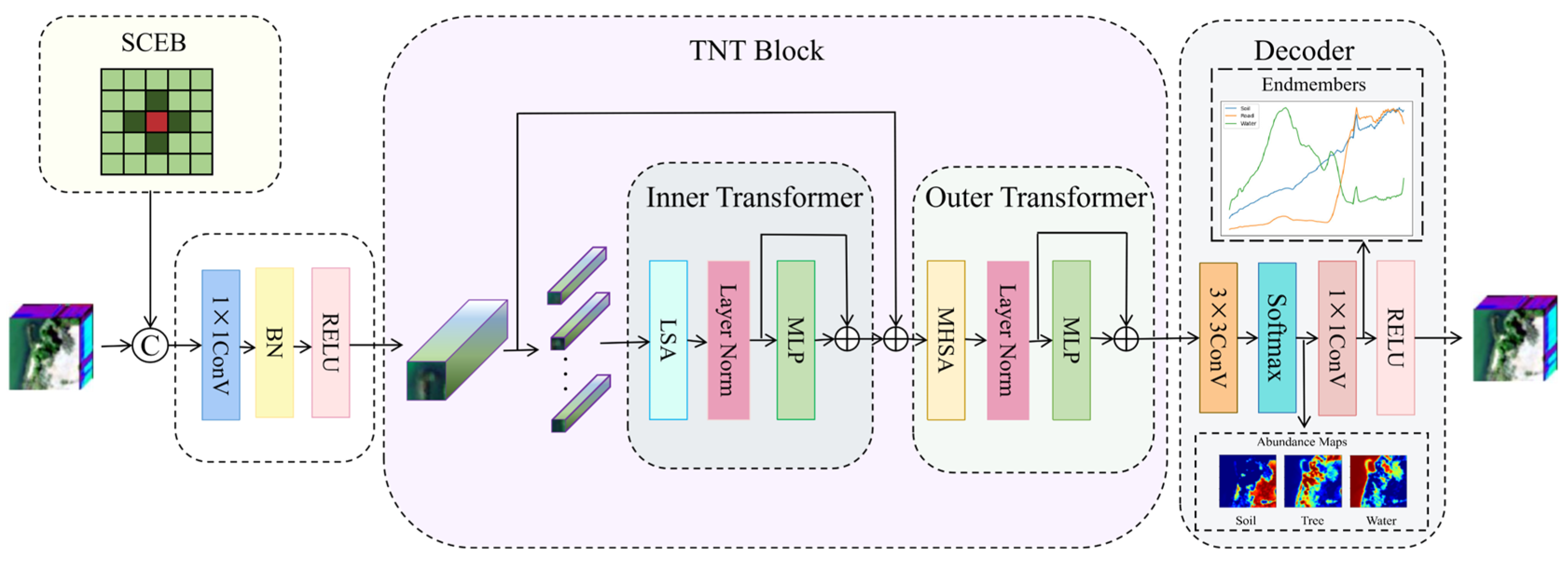
This section provides a detailed description of the proposed hyperspectral unmixing framework, termed SSTNT (Spatial–Spectral Similarity guided Transformer-in-Transformer with Linear Self-Attention). As illustrated in Figure 1, the overall architecture consists of a SCEB module, a TNT encoder, a linear self-attention mechanism, and decoding and constraint modules.

3.1. SCEB Module

Pixels in hyperspectral images often exhibit strong spatial continuity, and adjacent pixels typically share highly similar spectral characteristics. If neighborhood relationships are neglected, the resulting abundance maps are prone to noise artifacts or spatial discontinuities [43]. Cosine similarity is effective for material discrimination based on spectral shape; however, when different materials exhibit highly similar spectral shapes, cosine similarity alone may not provide sufficient discriminative power [44]. In such cases, the Euclidean distance between the input spectrum and the endmember spectrum can effectively reflect amplitude variations induced by intrinsic material properties, facilitating the capture of absolute intensity differences and thereby improving unmixing accuracy [45]. Traditional methods often rely on a single similarity metric, making it difficult to simultaneously account for both spectral shape and intensity information, which limits their ability to distinguish spectrally similar pixels in complex scenes. Therefore, motivated by the two fundamental characteristics of hyperspectral data, spectral shape similarity and amplitude consistency, a similarity module is introduced at the input stage. This module jointly exploits cosine similarity and Euclidean distance to construct a similarity tensor that comprehensively characterizes the spectral relationships among pixels.

Specifically, for a central ${\mathrm{x}}_{\mathrm{i}}$ pixel in the input hyperspectral image and its neighboring pixel ${\mathrm{x}}_{\mathrm{j}}$, both the cosine similarity and the Euclidean distance are computed simultaneously:

$$d_c\left(x_i,x_j\right)=\cos \left(x_i,x_j\right)={\displaystyle \frac{x_i^{\top }{x}_j}{\Vert x_i{\Vert }_2\Vert x_j{\Vert }_2}}$$

(7)

$$d_e\left(x_i,x_j\right)=\Vert x_i-x_j{\Vert }_2=\sqrt{{\displaystyle \sum _{k=1}^L{\left(x_{i,k}-x_{j,k}\right)}^2}}$$

(8)

where $\Vert \cdot {\Vert }_2$ denotes the Euclidean norm, and $x_{i,k}$, $x_{j,k}$ represent the spectral values of pixels $x_i$ and $x_j$ at the k-th spectral band, respectively. A cosine similarity value closer to 1 indicates higher spectral shape similarity between two pixels, while a smaller Euclidean distance implies a smaller spectral discrepancy. By combining these two complementary similarity measures, a comprehensive spectral similarity between pixels is obtained.

To this end, a weighted formulation is adopted to generate the similarity tensor $S_{i,j}$, which represents the similarity between pixels $x_i$ and $x_j$, defined as:

$${\mathrm{S}}_{\mathrm{i},\mathrm{j}}={\mathrm{d}}_{\mathrm{c}}({\mathrm{x}}_{\mathrm{i}},{\mathrm{x}}_{\mathrm{j}})+\mathrm{e}\mathrm{x}\mathrm{p}(-{\displaystyle \frac{{\mathrm{d}}_{\mathrm{e}}({\mathrm{x}}_{\mathrm{i}},{\mathrm{x}}_{\mathrm{j}})}{\mathrm{\sigma }}})$$

(9)

Through this similarity tensor, neighborhood information is constructed for each pixel and introduced as a structural prior, enabling the model to adapt to different regional spectral distributions. In regions with higher similarity, abundance distributions tend to be sparser, whereas in regions with lower similarity, abundance distributions become smoother. This adaptive behavior allows the unmixing process to more accurately capture region-specific characteristics.

The similarity tensor generated by this module is concatenated with the original hyperspectral image along the channel dimension and subsequently fed into the improved Transformer-in-Transformer (TNT) network after dimensionality reduction via a 1 × 1 convolution, followed by batch normalization (BN) and ReLU activation. This design facilitates a deep fusion of spectral and spatial information.

3.2. Linear Self-Attention Mechanism

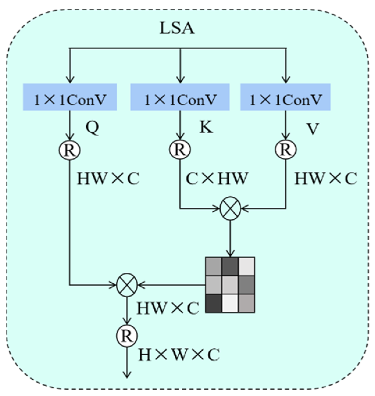
In the proposed framework, Linear Self-Attention (LSA) serves as the core module of the inner Transformer, aiming to efficiently capture local spatial–spectral dependencies. As illustrated in Figure 2, the input to the LSA module is the fused feature representation $X_{fusion}\in {\mathbb{R}}^{H\times W\times C}$, which is obtained by concatenating the similarity tensor produced by the similarity module with the original hyperspectral image, followed by dimensionality reduction using a 1 × 1 convolution.

First, three 1 × 1 convolutional layers are employed to generate the query, key, and value matrices Q, K, and V, respectively:

$$\left\{\begin{array}{l}Q=H_{conv}^Q\left(X_{fusion}\right)\hfill \\ K=H_{conv}^K\left(X_{fusion}\right)\hfill \\ V=H_{conv}^V\left(X_{fusion}\right)\hfill \end{array}\right.$$

(10)

where the convolutional operations perform feature projections along the spectral dimension without altering the spatial resolution.

The core computation of LSA is defined as:

$$Attention\left(Q,K,V\right)=Q\left(S\left({\displaystyle \frac{K^{\top }}{\sqrt{d}}}\right)V\right)$$

(11)

where $S\left(\cdot \right)$ denotes the Softmax function and d is the scaling factor corresponding to the feature dimensionality. The key idea of this formulation lies in reordering the computation sequence: instead of explicitly computing the full attention matrix, $S\left({\displaystyle \frac{K^{\top }}{\sqrt{d}}}\right)V$ is calculated first, followed by multiplication with Q. This reformulation effectively reduces the computational complexity of conventional self-attention from $O\left(N^2\right)$ to $O\left(N\right)$.

As shown in

Table 1. Quantitative evaluation of computational complexity for MHSA and LSA.

Window Size	MHSA FLOPs (MFLOPs)	LSA FLOPs (MFLOPs)	MHSA Time (ms)	LSA Time (ms)	MHSA Memory (MB)	LSA Memory (MB)
4 × 4	0.27	0.27	0.458	0.480	9.28	9.31
5 × 5	0.42	0.41	0.520	0.530	9.43	9.35
8 × 8	1.10	1.06	0.480	0.570	9.54	9.52
16 × 16	4.98	4.24	0.458	0.510	10.63	11.07
24 × 24	13.42	9.55	0.980	0.650	19.07	16.28
32 × 32	29.36	16.97	2.610	0.510	41.25	28.51
64 × 64	268.42	67.90	38.804	0.936	524.38	278.38

, when the window size is small (e.g., 4 × 4), the computational cost of LSA is comparable to that of MHSA. However, as the window size increases, the computational burden of MHSA grows rapidly. When the window size reaches 64 × 64 (4096 tokens), MHSA requires 268.42 MFLOPs and 39.80 ms inference time, while LSA requires 67.90 MFLOPs and 0.94 ms. Meanwhile, GPU memory consumption is reduced from 524.38 MB to 278.38 MB. In the proposed SSTNT framework, the window size is set to 5 × 5, which is consistent with the patch size in the inner Transformer.

Finally, the output of the LSA module is reshaped back to the original spatial dimensions:

$$H_{LSA}\left(X_{fusion}\right)=H_{r\mathrm{e}shape}^{-1}\left(Attention\left(Q,K,V\right)\right)$$

(12)

Through this linear self-attention mechanism, the model not only efficiently captures local spectral similarity and spatial dependencies, but also preserves fine-grained regional details under a computationally tractable cost.

3.3. Modified Transformer-in-Transformer (TNT) Encoder

Transformers exhibit excellent capability in global modeling; however, when applied to high-resolution hyperspectral images (HSIs), they suffer from two major limitations: insufficient capture of local spatial details and high computational complexity of window-based attention. The Transformer-in-Transformer (TNT) framework addresses these issues by introducing a dual-token mechanism, in which interactions between inner tokens and outer tokens enable effective modeling of both local and global information.

In the TNT framework, the input image is first partitioned into a set of patch tokens, and each patch is further subdivided into smaller sub-patches. The outer Transformer operates at the patch level, focusing on global information modeling by capturing long-range dependencies among different patches and integrating global contextual information to maintain overall image coherence. In contrast, the inner Transformer concentrates on fine-grained pixel-level information within each patch, capturing local spectral characteristics and spatial relationships to preserve detailed local structures. Through the interaction between inner and outer tokens, TNT is able to jointly attend to local details and global semantics, thereby achieving multi-scale feature modeling.

Suppose that the input hyperspectral image is uniformly divided into n patches, denoted as:

$$X=\left[X_1,X_2,\dots ,X_n\right]\in {\mathbb{R}}^{n\times p\times p\times C}$$

(13)

where $X_i$ represents the input feature of the i-th patch, n is the number of patches, p denotes the spatial size of each patch, and C is the number of spectral bands.

Each patch is further subdivided into m sub-patches, denoted as:

$$X^{\prime }\to \left[X_{i,1},X_{i,2},\dots X_{i,m}\right]$$

(14)

where $X_{i,j}\in {\mathbb{R}}^{s\times s\times C}$ represents the feature of the j-th sub-patch within the i-th patch, and s denotes the spatial size of each sub-patch.

By vectorization and linear projection, the sub-patch features are transformed into a sequence of token embeddings:

$$Y_i=\left[y_{i,1},y_{i,2},\dots ,y_{i,m}\right], y_{i,j}=FC\left(Vec\left(x_{i,j}\right)\right)$$

(15)

where $Y_i$ denotes the token representation of all sub-patches within the i-th patch, $y_{i,j}\in {\mathbb{R}}^c$ is the token corresponding to the j-th sub-patch, c is the embedding dimension of the sub-patch tokens, FC is a fully connected layer, and $Vec\left(\cdot \right)$ denotes the vectorization operator that reshapes a spatial feature map into a one-dimensional vector by flattening its spatial dimensions.

For the sub-patch token sequences, an inner Transformer is employed to model fine-grained local relationships within each patch. The computation of the inner Transformer is given by:

$${Y^{\prime }}_i^l=Y_i^{l-1}+LSA\left(LN\left(Y_i^{l-1}\right)\right)$$

(16)

$$Y_i^l={Y^{\prime }}_i^l+MLP(LN\left({Y^{\prime }}_i^l\right))$$

(17)

where $l=1,2,\dots ,L$ denotes the index of the Transformer layer, L is the total number of inner Transformer layers, $LSA\left(\cdot \right)$ denotes the linear self-attention mechanism, $LN\left(\cdot \right)$ is layer normalization, and $MLP\left(\cdot \right)$ represents a feed-forward network. This process aggregates detailed intra-patch information and provides high-quality local semantic representations for subsequent global modeling.

To capture global relationships among patches, the patch-level token sequence is defined as:

$$Z^0=\left[Z_{class},Z_1^0,Z_2^0,\dots ,Z_n^0\right]\in {\mathbb{R}}^{\left(n+1\right)\times d}$$

(18)

where $Z_{class}$ is a learnable class token, and $Z_i^0$ denotes the initial token of the i-th patch.

At each layer, the features learned by the inner Transformer from the sub-patches are projected via a linear transformation and added to the corresponding patch-level token representation.

$$Z_i^{l-1}=Z_i^{l-1}+FC\left(Vec\left(Y_i^l\right)\right)$$

(19)

where $Z_i^{l-1}\in {\mathbb{R}}^d$. Through this additive operation, the patch representation effectively integrates both the original structural information and the locally enhanced semantic features.

Subsequently, the outer Transformer updates the patch-level token sequence as follows:

$${{\mathrm{Z}}^{\prime }}^{\mathrm{l}}={\mathrm{Z}}^{\mathrm{l}-1}+\mathrm{M}\mathrm{H}\mathrm{S}\mathrm{A}(\mathrm{L}\mathrm{N}({\mathrm{Z}}^{\mathrm{l}-1}))$$

(20)

$$Z^l={Z^{\prime }}^l+MLP\left(LN{Z^{\prime }}^l\right))$$

(21)

It is used to capture the long-range dependencies among different patches and achieve global feature modeling.

In summary, a TNT block jointly updates both sub-patch and patch representations, which can be expressed as:

$$\left(Y^l,Z^l\right)=TNT\left(Y^{l-1},Z^{l-1}\right)$$

(22)

Compared with the conventional Transformer architecture, the TNT framework exhibits significant advantages. First, by employing nested inner and outer Transformers, it enables hierarchical feature extraction, allowing information learning from local to global scales in a more effective manner. Second, TNT reduces computational complexity: compared with the $O\left(N^2\right)$ complexity of standard Transformers, the TNT complexity is reduced to $O\left(N+M^2\right)$, which significantly alleviates the computational burden when processing high-resolution images.

To preserve spatial information, learnable one-dimensional positional embeddings are added to both patch and sub-patch tokens. The patch-level positional encoding is defined as:

$$Z^0\leftarrow Z^0+E_{\mathit{patch}}, E_{\mathit{patch}}\in {\mathbb{R}}^{\left(n+1\right)\times d}$$

(23)

and the sub-patch positional encoding is defined as:

$$Y^0\leftarrow Y_i^0+E_{\mathit{subpacth}}, E_{\mathit{subpatch}}\in {\mathbb{R}}^{m\times c}, i=1,2,\dots n$$

(24)

This design preserves global spatial consistency while maintaining local relative positional relationships.

In our implementation, the input hyperspectral image is uniformly partitioned into fixed-size patches of 5 × 5, resulting in 25 sub-patch tokens (pixel-level inner tokens) within each patch. The sub-patch size corresponds to a 1 × 1 pixel, meaning that each pixel inside a patch is treated as an individual inner token for fine-grained local modeling. These structural hyperparameters are kept consistent across all datasets and are not tuned per dataset, ensuring architectural consistency and experimental fairness.

3.4. Decoder

The feature representations output by the TNT module denoted as $F_{TNT}=\mathrm{Re}shape\left(Z^l\right)\in {\mathbb{R}}^{H\times W\times C}$ are first passed through a 3 × 3 convolutional layer to integrate local contextual information and reconstruct the feature maps:

$$H_{dec}=Con{v}_{3\times 3}\left(F_{TNT}\right)$$

(25)

Subsequently, a 1 × 1 convolutional layer is applied to project the channel dimension to the number of endmembers P, thereby generating the abundance maps $A\in {\mathbb{R}}^{H\times W\times P}$:

$$A=Con{v}_{1\times 1}\left(H_{dec}\right)$$

(26)

To satisfy the physical constraints of hyperspectral unmixing, namely non-negativity and the sum-to-one constraint, a Softmax function is applied along the channel dimension to normalize the abundance distribution of each pixel:

$${\widehat{A}}_{ij}={\displaystyle \frac{\exp \left(A_{ij}\right)}{{\displaystyle \sum _{P=1}^P\exp \left(A_{ip}\right)}}}$$

(27)

After abundance estimation, the model performs linear spectral reconstruction using a trainable endmember matrix $\widehat{E}\in {\mathbb{R}}^{P\times C}$:

$$\widehat{X}=\widehat{A}\widehat{E}$$

(28)

where $\widehat{X}$ denotes the reconstructed hyperspectral image and $\widehat{E}$ represents the estimated endmember spectra learned by the network.

The endmember matrix is learned in an end-to-end manner without requiring a predefined spectral library, which not only preserves the physical interpretability of the unmixing process but also enables adaptive spectral representation learning.

3.5. Loss Function

To improve the accuracy of endmember extraction and abundance estimation, a joint loss function is designed in this work, which is defined as:

$$\mathcal{L}={\mathcal{L}}_{MSE}+\lambda {\mathcal{L}}_{SAD}$$

(29)

where λ is a balancing coefficient that controls the trade-off between spectral amplitude differences and spectral shape discrepancies.

The Mean Squared Error (MSE) loss is employed to minimize the discrepancy between the reconstructed spectra and the ground-truth spectra, and is defined as:

$${\mathcal{L}}_{MSE}={\displaystyle \frac{1}{N}}{\displaystyle \sum _{i=1}^N\Vert X_i-{\widehat{X}}_i{\Vert }_2^2}$$

(30)

where $X_i$ denote the ground-truth and reconstructed spectra of the i-th pixel, respectively, and N is the total number of pixels.

The Spectral Angle Distance (SAD) loss emphasizes spectral shape similarity and is introduced to enhance endmember purity. It is formulated as:

$${\mathcal{L}}_{SAD}={\displaystyle \frac{1}{N}}{\displaystyle \sum _{i=1}^N\arccos \frac{X_i\cdot {\widehat{X}}_i}{\Vert X_i{\Vert }_2\Vert {\widehat{X}}_i{\Vert }_2}}$$

(31)

4. Experiments

To ensure the validity of the experimental evaluation, experiments were conducted on one synthetic dataset and three real-world datasets, namely Samson, Jasper Ridge, and Apex. The RGB visualizations of these four datasets are shown in Figure 3. The superiority of the proposed method is verified through comprehensive comparisons with eight representative hyperspectral unmixing approaches, including A2SAN [23], DFFN [24], CyCU [22], MAT-Net [37], TCCU [36], CDCTA [25], DeepTrans [31], and MOGNMF [46].

4.1. Datasets

• Synthetic dataset [47]: The synthetic dataset consists of 60 × 60 pixels with 200 spectral bands covering the spectral range of 0.4–1.4 μm. In this dataset, one material is used as the background, while the remaining four materials are distributed at the four corners of the scene. The abundance values are generated according to a Dirichlet distribution. The dataset includes five endmembers: Asphalt, Conifer, Concrete, Basalt, and Limestone.
• Samson dataset [48]: The Samson dataset contains 952 × 952 pixels with 156 spectral bands ranging from 401 to 889 nm. A 95 × 95 subregion is extracted starting from pixel location (252, 332). The dataset mainly consists of three endmembers: Soil, Tree, and Water.
• Jasper Ridge dataset [49]: The Jasper Ridge dataset comprises 512 × 614 pixels with 224 spectral bands covering the spectral range from 380 to 2500 nm. A 100 × 100 subregion is extracted starting from pixel location (105, 269). The final dataset includes four endmembers: Tree, Soil, Water, and Road.
• Apex dataset [50]: The Apex dataset consists of 110 × 110 pixels with 285 spectral bands ranging from 413 to 2420 nm. This dataset contains four endmembers: Water, Tree, Road, and Roof.

4.2. Evaluation Metrics

In this comparative experiment, three widely used evaluation metrics are adopted to assess the performance of the proposed model: the reconstruction error (RE) between the reconstructed spectra and the original spectra, the root mean square error (RMSE) between the estimated abundances and the ground-truth abundances, and the spectral angle distance (SAD) between the estimated endmembers and the reference endmember signatures. These metrics are defined as follows:

$$RE\left(X,\widehat{X}\right)={\displaystyle \frac{1}{N}}{\displaystyle \sum _{j=1}^{N}RE\left(x_j,{\widehat{x}}_j\right)}$$

(32)

$$RMSE\left({\widehat{a}}_j,a_j\right)=\sqrt{{\displaystyle \frac{1}{N}}{\displaystyle \sum _{j=1}^N{\left({\widehat{a}}_j-a_j\right)}^2}}$$

(33)

$$SAD\left(e_m,{\widehat{e}}_m\right)=\arccos {\displaystyle \frac{e_m\cdot {\widehat{e}}_m}{\Vert e_m{\Vert }_2\Vert {\widehat{e}}_m{\Vert }_2}}$$

(34)

where ${\widehat{x}}_j,{\widehat{a}}_j,{\widehat{e}}_m$ denote the estimated spectral image, abundance maps, and endmember signatures, respectively, while $x_j,a_j,e_m$ represent the corresponding ground-truth spectral image, abundance maps, and endmember signatures.

4.3. Experimental Settings and Hyperparameter Analysis

All experiments were conducted on a computer equipped with an Intel(R) Core(TM) i5-10210U CPU and an NVIDIA GeForce MX250 GPU, using Python 3.10 as the software environment. Figure 4, Figure 5 and Figure 6 illustrate the hyperparameter analysis results on different datasets. As shown in Figure 4, the model achieves optimal performance on the Samson dataset when the learning rate is set to 9 × 10⁻³ and the parameters β and γ are set to 8 × 10⁴ and 1 × 10⁻², respectively. Figure 5 demonstrates that on the Jasper Ridge dataset, the best performance is obtained with a learning rate of 5 × 10⁻⁴, β = 1 × 10², and γ = 1 × 10⁻². As illustrated in Figure 6, for the Apex dataset, the optimal performance is achieved when the learning rate is set to 1 × 10⁻², with β = 1 × 10² and γ = 1 × 10⁻². In addition,

Table 2. Network hyperparameter settings.

Parameters	Synthetic	Samson	Jasper Ridge	Apex
Learning rate	1 × 10−3	9 × 10−3	5 × 10−4	1 × 10−2
β	9 × 104	9 × 104	1 × 102	1 × 102
γ	1 × 10−2	1 × 10−2	1 × 10−2	1 × 10−3
Epoch	600	200	200	200
Weight decay	5 × 10−5	4 × 10−5	1 × 10−5	3 × 10−5
Dim	200	300	200	200

provides detailed training parameter configurations.

4.4. Robustness Analysis

To evaluate robustness under noisy conditions, Gaussian noise with SNR levels of 30 dB, 20 dB, and 10 dB were added to the synthetic dataset. The spatial distribution was kept unchanged to ensure a controlled comparison.

Table 3. Quantitative evaluation under varying SNR conditions on the synthetic dataset.

SNR (dB)	RE	Mean RMSE	Mean SAD
10	0.03331765	0.06354388	0.02985694
20	0.01105196	0.01940381	0.00706320
30	0.00481180	0.01752950	0.00400321

reports the quantitative results under different noise levels. As the SNR decreases, RE, mean RMSE, and mean SAD increase gradually, which is consistent with the expected impact of stronger noise interference. Even under the challenging 10 dB condition, the proposed SSTNT maintains stable reconstruction performance without severe degradation. These results indicate that the proposed framework exhibits reliable robustness under varying noise levels.

Although the above experiments evaluate robustness under additive Gaussian noise, real hyperspectral imaging scenarios may also involve spectral variability induced by illumination changes and environmental conditions. Such variability may influence similarity estimation, especially when spectral responses of identical materials exhibit spatially varying amplitude or shape deviations. In the proposed framework, the joint use of cosine similarity and Gaussian-weighted Euclidean distance provides partial tolerance to moderate variability, while the hierarchical contextual modeling of the Transformer helps mitigate local perturbations. Nevertheless, the current model does not explicitly incorporate variability-aware mixing formulations such as ELMM or ALMM. Exploring such integration constitutes an important direction for future work.

4.5. Experimental Results and Comparisons

(1)

Synthetic dataset: The quantitative experimental results on the Synthetic dataset are reported in

Table 4. Average RMSE results on the Synthetic dataset. The best performances are shown in bold.

	A2SAN	DFFN	CyCU	MAT-Net	TCCU	CDCTA	DeepTrans	MOGNMF	Proposed
Asphalt	0.070564	0.021701	0.212267	0.019836	0.178095	0.124731	0.077719	0.301419	0.018146
Conifer	0.037345	0.032438	0.075195	0.010716	0.045452	0.044407	0.02266	0.2117	0.006401
Concrete	0.025244	0.012506	0.202546	0.011472	0.086241	0.063809	0.039133	0.164475	0.010372
Basalt	0.022575	0.020398	0.06019	0.005372	0.02925	0.115353	0.012115	0.15707	0.004079
Limestone	0.024246	0.045757	0.078678	0.010504	0.051927	0.099183	0.025527	0.216733	0.004084
Mean RMSE	0.035995	0.02656	0.12578	0.011580	0.094629	0.094599	0.042151	0.216502	0.010111

and

Table 5. Average SAD results on the Synthetic dataset. The best performances are shown in bold.

	A2SAN	DFFN	CyCU	MAT-Net	TCCU	CDCTA	DeepTrans	MOGNMF	Proposed
Asphalt	0.017853	0.025443	0.038516	0.010276	0.106838	0.012836	0.013716	0.097935	0.005699
Conifer	0.028957	0.018164	0.02366	0.007337	0.002966	0.008621	0.014773	0.003665	0.003032
Concrete	0.015623	0.013012	0.037079	0.006673	0.015978	0.016285	0.020274	0.005939	0.010160
Basalt	0.007343	0.011846	0.02762	0.004231	0.014222	0.018939	0.009475	0.007611	0.003109
Limestone	0.014051	0.010555	0.023848	0.005850	0.004244	0.005796	0.005181	0.002206	0.002154
Mean SAD	0.016765	0.015804	0.03015	0.006873	0.028849	0.012495	0.012684	0.023471	0.004830

. It can be observed that the proposed SSTNT method achieves the best overall performance in both abundance estimation and endmember extraction. Specifically, SSTNT attains an average RMSE of 0.01011 for abundance estimation. In terms of endmember extraction, SSTNT achieves an average SAD of 0.00843, which is significantly lower than those of the competing methods. Overall, SSTNT demonstrates superior performance in both abundance estimation and endmember extraction on the Synthetic dataset.

(2)

Samson dataset: The quantitative results on the Samson dataset are presented in

Table 6. Average RMSE results on the Samson dataset. The best performances are shown in bold.

	A2SAN	DFFN	CyCU	MAT-Net	TCCU	CDCTA	DeepTrans	MOGNMF	Proposed
Soil	0.293396	0.170557	0.094999	0.131851	0.070389	0.116132	0.066872	0.133577	0.048273
Tree	0.178938	0.280304	0.091981	0.124031	0.089077	0.061404	0.068753	0.134266	0.040824
Water	0.156054	0.166506	0.114073	0.209123	0.060503	0.11185	0.078736	0.197047	0.021098
Mean RMSE	0.209463	0.205789	0.10035	0.155002	0.074274	0.099611	0.071643	0.157795	0.038479

and

Table 7. Average SAD results on the Samson dataset. The best performances are shown in bold.

	A2SAN	DFFN	CyCU	MAT-Net	TCCU	CDCTA	DeepTrans	MOGNMF	Proposed
Soil	0.099042	0.011232	0.025898	0.017577	0.018725	0.025516	0.008788	0.059	0.019794
Tree	0.061059	0.085242	0.09576	0.094066	0.087918	0.076929	0.055524	0.079612	0.057404
Water	0.057895	0.077455	0.155353	0.052464	0.128033	0.046988	0.088204	0.11255	0.066152
Mean SAD	0.072665	0.057977	0.09234	0.054702	0.078225	0.049811	0.050838	0.08372	0.047783

. Compared with other methods, SSTNT achieves the lowest average RMSE and average SAD, indicating the best overall performance in abundance estimation. Specifically, SSTNT achieves an average RMSE of 0.038479, which is 0.033164 lower than that of the second-best method, DeepTrans. Moreover, its average SAD is 0.047783, outperforming the second-best method, CDCTA, by 0.002028.

(3)

Jasper Ridge dataset: The quantitative results on the Jasper Ridge dataset are shown in

Table 8. Average RMSE results on the Jasper Ridge dataset. The best performances are shown in bold.

	A2SAN	DFFN	CyCU	MAT-Net	TCCU	CDCTA	DeepTrans	MOGNMF	Proposed
Tree	0.117821	0.091505	0.146411	0.092519	0.141819	0.207404	0.098407	0.13636	0.062798
Water	0.097616	0.12764	0.239143	0.092593	0.110187	0.106293	0.106593	0.036376	0.069435
Soil	0.143171	0.022827	0.142267	0.092802	0.140365	0.279079	0.075827	0.155773	0.075738
Road	0.12455	0.059034	0.288608	0.079496	0.115388	0.244931	0.058947	0.105436	0.064028
Mean RMSE	0.120790	0.075252	0.20411	0.089352	0.127740	0.219198	0.086992	0.117579	0.068192

and

Table 9. Average SAD results on the Jasper Ridge dataset. The best performances are shown in bold.

	A2SAN	DFFN	CyCU	MAT-Net	TCCU	CDCTA	DeepTrans	MOGNMF	Proposed
Tree	0.126583	0.045067	0.090107	0.090409	0.145768	0.044338	0.101541	0.140461	0.089083
Water	0.113232	0.084453	0.090061	0.082193	0.121577	0.149058	0.157014	0.114126	0.089702
Soil	0.083907	0.088783	0.116542	0.062417	0.109088	0.209606	0.032076	0.082422	0.048761
Road	0.111619	0.077529	0.148142	0.054140	0.048636	0.122741	0.023632	0.043674	0.040064
Mean SAD	0.108835	0.073958	0.11121	0.072290	0.106267	0.131436	0.078566	0.095171	0.066903

. SSTNT consistently achieves the lowest average RMSE and average SAD among all compared methods. In abundance estimation, SSTNT obtains an average RMSE of 0.06819, which is 27.5% lower than that of the second-best method, DeepTrans, and demonstrates the best performance in estimating tree abundances. For endmember extraction, SSTNT achieves an average SAD of 0.066903, outperforming the second-best method, MAT-Net, by 8.05%.

(4)

Apex dataset: The quantitative results on the Apex dataset are reported in

Table 10. Average RMSE results on the Apex dataset. The best performances are shown in bold.

	A2SAN	DFFN	CyCU	MAT-Net	TCCU	CDCTA	DeepTrans	MOGNMF	Proposed
Road	0.110542	0.215369	0.272744	0.459612	0.196648	0.213874	0.163574	0.176849	0.176605
Roof	0.16899	0.186881	0.185287	0.309714	0.156618	0.128569	0.097246	0.13505	0.101329
Tree	0.151174	0.170192	0.168676	0.223468	0.132509	0.141333	0.1277	0.115242	0.125194
Water	0.134618	0.127242	0.11544	0.180242	0.127859	0.109206	0.116225	0.111244	0.077475
Mean RMSE	0.141331	0.174921	0.18554	0.293259	0.155809	0.153438	0.12848	0.137085	0.125631

and

Table 11. Average SAD results on the Apex dataset. The best performances are shown in bold.

	A2SAN	DFFN	CyCU	MAT-Net	TCCU	CDCTA	DeepTrans	MOGNMF	Proposed
Road	0.096538	0.393908	0.685528	0.691465	0.097591	0.161311	0.129256	0.116489	0.075274
Roof	0.051664	0.573077	0.230815	0.224342	0.132261	0.142887	0.132241	0.1395506	0.132443
Tree	0.107419	0.05117	0.122334	0.116203	0.089109	0.192442	0.096667	0.082343	0.083194
Water	0.128747	0.138322	0.508118	0.2310007	0.058609	0.037116	0.046294	0.052472	0.043344
Mean SAD	0.096092	0.289119	0.3867	0.315752	0.094392	0.133439	0.101114	0.097714	0.08356

. As can be observed, SSTNT achieves the lowest average RMSE and average SAD compared with all competing methods. Specifically, SSTNT obtains an average RMSE of 0.12563 in abundance estimation, which is 2.26% lower than that of the second-best method, DeepTrans, and exhibits the best performance in estimating water abundances. In terms of endmember extraction, SSTNT achieves an average SAD of 0.08356, which is 12.96% lower than that of the second-best method, MOGNMF, demonstrating superior performance in extracting road and water endmembers.

4.6. Visual Analysis

Figure 7 and Figure 8 visually present the estimated endmember signatures and abundance maps obtained by all unmixing methods on the Synthetic dataset. As shown in Figure 7, the abundance maps produced by SSTNT, MAT-Net, and TCCU are closer to the ground truth (GT) compared with other methods. Figure 8 illustrates the endmember estimation results, where the endmembers extracted by SSTNT, MAT-Net, and TCCU are almost identical to the ground-truth signatures.

Figure 9 and Figure 10 further present qualitative comparisons of the abundance maps and endmember spectra of the Samson dataset. As shown in Figure 9, the abundance maps generated by SSTNT are closer to the ground truth and better preserve spatial continuity and the boundary structures of land-cover regions. This consistency can be attributed to SSTNT’s effective modeling of spatial–spectral similarity, which enables the capture of intrinsic relationships among materials across multiple spatial scales, thereby allowing a more accurate characterization of abundance variations in mixed pixels. In contrast, methods such as CDCTA and MOGNMF tend to underestimate the abundances of sand and water, resulting in incomplete local structures or unnecessary detail noise in the corresponding abundance maps. Figure 10 further indicates that the endmember spectra estimated by SSTNT is almost completely consistent with the reference spectra.

Figure 11 and Figure 12 present qualitative comparisons of unmixing results on the Jasper Ridge dataset. The abundance maps and endmember spectra generated by SSTNT exhibit significantly higher consistency with the ground truth than those of other methods. As shown in Figure 11, the abundance distributions produced by SSTNT maintain high consistency with the reference abundance maps (GT) in terms of spatial structure and detail representation, particularly in regions dominated by Tree, Soil, and Road materials, where abundance variations are more continuous and boundaries are more clearly delineated. In contrast, some competing methods exhibit noticeable estimation biases: MAT-Net tends to overestimate water abundance in water-dominated regions while underestimating tree and road abundances to varying degrees; CyCU shows insufficient detail representation in soil abundance maps, leading to excessive smoothing of local structures. Meanwhile, DeepTrans and MOGNMF exhibit varying degrees of underestimation in water abundance, resulting in a loss of critical spatial details. In comparison, SSTNT effectively mitigates these issues and maintains a more reasonable abundance allocation across different land-cover classes. Figure 12 shows the comparison between the estimated endmember spectra and the reference spectra, from which it can be observed that SSTNT achieves a high degree of consistency with the reference endmembers in both overall spectral trends and local band variations.

Figure 13 and Figure 14 present qualitative comparisons of unmixing results on the Apex dataset. The abundance maps and endmember spectra produced by SSTNT show significantly higher agreement with the ground truth than those generated by other methods. As illustrated in Figure 13, the abundance distributions generated by SSTNT maintain high consistency with the reference abundance maps in terms of spatial structure and detail representation, accurately capturing the spatial morphology and boundary information of Road, Tree, and Roof materials. In contrast, several competing methods exhibit varying degrees of estimation bias: A2SAN, DFFN, and MOGNMF generally overestimate water abundance in water-dominated regions while significantly underestimating road and tree abundances, leading to inaccurate spatial representations. MAT-Net and TCCU suffer from insufficient detail representation in roof abundance maps, with over-smoothed local regions that weaken boundary information. Furthermore, A2SAN, DFFN, CDCTA, and DeepTrans still exhibit varying degrees of water overestimation in road-dominated pixels, reducing spatial consistency in road regions. By contrast, SSTNT maintains a more balanced and reasonable abundance distribution across different land-cover classes, effectively alleviating the above issues. As shown in Figure 14, SSTNT achieves high consistency with the reference endmembers in terms of overall spectral trends and key band variations, accurately capturing the main characteristics of the endmember spectra.

4.7. Ablation Experiment

To verify the effectiveness and individual contributions of each component in the proposed SSTNT model, including the similarity module, the TNT framework, and the linear self-attention (LSA) module, comprehensive ablation experiments were conducted on four datasets. The quantitative results in terms of RMSE and SAD under different ablation settings are reported in

Table 12. Ablation experiment on our proposed SSTNT with varying information enhancement on different datasets. Best results are shown in bold. Note: √ denotes that the corresponding module is enabled, and × denotes that the module is disabled.

Module			Synthetic		Samson		Jasper Ridge		Apex
Similarity	TNT	LSA	RMSE	SAD	RMSE	SAD	RMSE	SAD	RMSE	SAD
√	√	√	0.010111	0.004830	0.038479	0.047783	0.068192	0.066903	0.125631	0.08356
×	√	√	0.031694	0.00611	0.068031	0.076351	0.069022	0.0808269	0.141821	0.224915
√	×	√	0.029098	0.008979	0.137113	0.0970139	0.076289	0.0869603	0.231061	0.297907
√	√	×	0.012853	0.006153	0.039927	0.067611	0.114466	0.076729	0.150966	0.129573
√	×	×	0.019337	0.006741	0.047174	0.0600001	0.075191	0.075028	0.1275802	0.113233

. Overall, the complete SSTNT model achieves the best performance across all four datasets in terms of both reconstruction error (RMSE) and spectral angle distance (SAD), demonstrating the effectiveness of the proposed framework. The contributions of individual modules are analyzed as follows:

(1)

Effectiveness of the SCEB module: The introduction of the similarity module that jointly integrates Euclidean distance and cosine similarity leads to a significant performance improvement. After removing the similarity module, the RMSE on the Samson dataset increases from 0.0385 to 0.0680, while the SAD rises from 0.0478 to 0.0764. Similarly, on the Apex dataset, the RMSE increases from 0.1256 to 0.1418. These results indicate that the similarity module effectively captures local spectral consistency among neighboring pixels through the complementary Euclidean–cosine dual-metric fusion mechanism. By explicitly incorporating neighborhood spectral correlations, the model becomes capable of distinguishing subtle differences among highly similar spectra, thereby improving abundance continuity and endmember discriminability.

(2)

Impact of the TNT architecture: The incorporation of the TNT framework substantially enhances the model’s capability for multi-level feature modeling. When the TNT module is replaced with a conventional Transformer, a pronounced performance degradation is observed. Specifically, the RMSE on the Jasper Ridge dataset increases from 0.0682 to 0.1371, and on the Apex dataset from 0.1256 to 0.2311. This clearly demonstrates that the dual-token mechanism of TNT—consisting of inner and outer tokens—plays a critical role in multi-scale feature extraction. In contrast, conventional Transformers rely solely on global attention across patch-level features and lack the ability to model fine-grained pixel relationships within patches, leading to a substantial loss in unmixing accuracy.

(3)

Contribution of linear self-attention (LSA): The adoption of LSA further improves the model’s ability to capture local details. When LSA is replaced with traditional multi-head self-attention (MHSA), the overall performance decreases. On the Jasper Ridge dataset, the RMSE increases from 0.0682 to 0.1145, while on the Apex dataset it rises from 0.1256 to 0.1510. In addition, the SAD values increase to varying degrees across all datasets. These results suggest that the LSA module is more effective in focusing on relevant neighboring pixels, thereby providing higher robustness and accuracy in both endmember extraction and abundance estimation.

5. Conclusions

This paper proposed a spatial–spectral similarity guided Transformer-in-Transformer hyperspectral unmixing framework (SSTNT). The similarity module enhances local spectral consistency by combining cosine similarity and Gaussian-weighted Euclidean distance, providing discriminative spatial–spectral representations. The improved TNT encoder achieves hierarchical feature modeling through inner–outer token interaction, while the linear self-attention mechanism reduces computational complexity and enables efficient global dependency modeling. Experimental results on synthetic and real hyperspectral datasets, including Samson, Jasper Ridge, and Apex, demonstrate that SSTNT achieves superior performance in terms of RMSE and SAD, with improved spatial smoothness and spectral consistency. Despite the promising results, several challenges remain in hyperspectral unmixing. Severe spectral variability may still affect robustness in complex scenes. In addition, integrating task-specific unmixing models with emerging foundation model-based representations could enhance cross-scene generalization. Future work will focus on improving robustness and scalability while exploring hybrid representation learning frameworks.