Abstract
High-order linear polarization (LP) modes and vortex beams carrying orbital angular momentum (OAM) are highly useful in various fields. High-order LP modes provide higher thresholds for nonlinear effects, reduced sensitivity to distortions, and better energy extraction in high-power lasers. OAM beams are useful in optical communication, imaging, particle manipulation, and fiber sensing. The ability to switch between these mode outputs enhances system versatility and adaptability, supporting advanced applications both in research and industry. This paper presents the design of a 19 × 1 photonic lantern capable of outputting 19 LP modes and 16 OAM modes with low loss. Using the beam propagation method, we simulated and analyzed the mode evolution process and insertion loss, and we calculated the transmission matrix of the photonic lantern. The results indicate that the designed device can efficiently evolve into these modes with a maximum insertion loss not exceeding 0.07 dB. Furthermore, an adaptive control system was developed by introducing a mode decomposition system at the output and combining it with the Stochastic Parallel Gradient Descent (SPGD) + basin hopping algorithm. Simulation results show that this system can produce desired modes with over 90% mode content, demonstrating promising application prospects in switchable high-order mode systems.
1. Introduction
High-order transverse modes exhibit significant utility across various fields. Specifically, in optical fibers, high-order linear polarization (LP) modes demonstrate higher thresholds for detrimental nonlinear effects, such as stimulated Brillouin scattering (SBS), compared to the fundamental mode [1]. These modes also exhibit reduced sensitivity to mode profile distortions and enhance energy extraction in high-power pulsed laser systems [2,3]. Additionally, high-order LP modes are indispensable in several critical applications, ranging from fiber sensors to gravitational wave detection, where they substantially mitigate thermal noise [4,5]. Vortex beams carrying orbital angular momentum (OAM) have also garnered increasing attention due to their potential applications in the optical communication [6,7], imaging, particle manipulation [8], and optical fiber sensing domains [3].
Over the past few decades, numerous methodologies for generating high-order modes have been explored, in both spatial systems [9,10] and all-fiber configurations [11,12,13,14,15]. All-fiber devices offer distinct advantages over spatial mode converters, including compact size and superior compatibility. Achieving all-fiber high-order mode conversion can be accomplished through techniques such as long-period fiber gratings (LPFGs) [11,12], mode-selective couplers (MSCs) [13], spatial light modulators (SLMs) [14], and photonic lanterns (PLs) [15].
The simplest photonic lanterns serve as spatial mode converters, seamlessly integrating single-mode signals from multiple individual waveguide cores into a single multimode waveguide. To achieve minimal loss operation, it is essential that the number of input single-mode fibers (SMFs) should equal the number of modes supported by the multimode fiber (MMF) [16]. These devices can be fabricated using either optical fibers or planar waveguides, offering versatile solutions for mode conversion in various optical systems. This capability makes photonic lanterns particularly valuable for applications requiring efficient coupling and manipulation of light modes in both fiber-based and integrated photonic platforms.
Photonic lanterns can be categorized into mode-selective photonic lanterns (MSPLs) and conventional photonic lanterns, each with distinct research focuses. For mode-selective photonic lanterns, which facilitate the conversion of optical signals from a single-mode input to specific higher-order modes at the output through meticulously optimized structural design, the process ensures precise and efficient mode transformation. Upon injecting light into one of the single-mode input ports, the signal traverses a tapered region where it is seamlessly integrated into a few designated on-demand modes. This process ultimately results in the emission of the precisely tailored high-order mode from the multimode output port. Characterized by ultra-low loss, large bandwidth, and high capacity, MSPLs play a pivotal role in mode conversion and multiplexing/demultiplexing, thereby enhancing the performance and versatility of optical systems. Eznaveh et al. demonstrated the selective excitation of LP11o, LP11e, LP21o, and LP21e modes using a five-core PL [15]. This study achieved insertion losses below 3 dB, showcasing the feasibility of precise mode selection in fiber-based systems. Velázquez-Benítez et al. fabricated a 15-core PL capable of multiplexing five LP mode groups, including radial high-order modes through microstructured templates [8]. Notably, LP31 and LP12 degenerated into one mode group, while LP41, LP22, and LP03 formed another. Chen et al. developed a low-loss, high-purity, and ultrabroadband all-fiber LP41 mode converter using fluorine-doped fibers [17,18]. By tapering a nine-core single-mode fiber bundle with an outer low-refractive-index capillary, they achieved selective excitation of the LP41e and LP41o modes. Zhao et al. modeled and demonstrated a self-matching photonic lantern designed to address the limitation of generating only three LP modes (LP01, LP11e, and LP11o) in a fiber laser [19]. G. Lopez-Galmiche et al. showcased a few-mode erbium-doped fiber amplifier that utilized a mode-selective photonic lantern to control the modal content of pump light [20,21]. This device supported six LP modes (LP01, LP11e, LP11o, LP21e, LP21o, and LP02), demonstrating the potential for enhanced amplification efficiency and signal quality in high-power applications. N. Wang et al. proposed and experimentally demonstrated an intra-cavity transverse mode-switchable fiber laser based on a mode-selective photonic lantern and a few-mode Er-doped fiber amplifier [6]. They showed that the six lowest-order LP modes could lase independently and were switchable by changing the input port of the photonic lantern, offering a new approach to dynamic mode switching in fiber lasers.
For conventional PLs, the desired mode can be achieved at the output by controlling the amplitude, phase, and polarization of the single-mode input arms. Combining with adaptive control algorithms, this approach enables dynamic adjustment and optimization of the output modes in real time [22,23,24,25,26,27,28,29]. Montoya et al. introduced a novel method utilizing a mode control system based on a photonic lantern to significantly mitigate thermal modal instability (TMI) [23,24]. This breakthrough highlighted the potential of photonic lanterns in improving the stability and performance of high-power fiber lasers. They also experimentally verified the efficacy of a 3 × 1 photonic lantern in mitigating TMI with a 25 µm core diameter fiber laser, achieving a steady 1.2 kW output [24]. Despite the small core diameter, this setup demonstrated the capability to control guided spatial modes effectively, even under high-power conditions. Lu et al. successfully generated low-power lower-order mode outputs and OAM mode outputs in a 50 µm core fiber using a 3 × 1 photonic lantern adaptive spatial mode control system [22]. Ze et al. employed a 3 × 1 photonic lantern-based adaptive spatial mode control system to achieve kilowatt-level operation in a 42 µm core fiber laser amplifier. By implementing this system, they obtained a stable, improved multi-mode performance towards single-mode operation, with an output of 1.08 kW and a beam quality factor M2 of 2.20 [28]. This study underscored the potential of photonic lanterns in high-power, large-mode-area fiber lasers but also highlighted the need for further research to address challenges such as thermal effects and SBS thresholds.
Despite the capability of photonic lanterns, whether MSPLs or conventional photonic lanterns, to output only some desired modes, they continue to leverage unique properties to address diverse technological challenges and enhance performance across multiple sectors. As for mode-selective photonic lanterns, they are restricted to outputting only a limited number of specific modes. In contrast, conventional photonic lanterns are generally limited to stably outputting the fundamental mode or a limited number of lower-order modes. Therefore, it is challenging for photonic lanterns to achieve the capability of outputting multiple high-order modes and enabling mode switching. Hence, investigating how to enhance the inherent mode conversion capabilities of photonic lanterns to support a diverse range of high-order modes and facilitate seamless mode switching, and integrating these capabilities into fiber laser systems, remains a topic of significant research importance.
This paper is organized as follows: Section 2 provides a detailed description of the methodology employed in the simulations, which covers the specific methods used for the photonic lantern design simulations and the control flow required for adaptive control. Section 3 presents the simulation results of the 19 × 1 photonic lantern, showcasing the successful generation of 19 LP modes and 16 OAM modes using the adaptive control program; it also delves into practical considerations and experimental outlooks necessary for achieving this functionality, offering a pathway from simulation to practical implementation. Finally, in the conclusion, we summarize the main findings of the study and provide insights into future research directions.
2. Methodology
2.1. Photonic Lantern as Adiabatic Mode Converter
Photonic lanterns evolve into the desired modes by gradually fusing the optical fields within multiple specifically arranged single-mode fibers in a tapered region. To maximize the confinement of energy within the guided modes of the single-mode beams and minimize energy dissipation through radiation modes in the cladding, it is essential to design a photonic lantern such that the tapering region of the single-mode fiber bundle satisfies the adiabatic transition condition. Adiabatic transition refers to the requirement that the change in the transverse dimensions of the single-mode fiber bundle within the tapering region must occur sufficiently slowly to ensure minimal mode coupling and energy loss, that is, satisfying the condition expressed by the equation:
where r is the radial radius, z is the axial distance, and and are the propagation constants of the two modes within the tapered single-mode fiber bundle that could potentially couple energy.
Beam propagation methods (BPMs) are widely used for modeling various guided wave devices [30]. Efficient nonuniform schemes, based on the generalized Douglas (GD) scheme, have been developed for the finite-difference beam propagation method (FD-BPM) [31]. These schemes enhance the accuracy and efficiency of simulations by adapting to the varying properties of the medium through which light propagates. The FD-BPM is particularly suitable for calculating the evolution of optical fields within photonic lanterns, where precise control over mode conversion and propagation is critical. This method allows for detailed analysis of the mode evolution process and insertion loss, facilitating the design and optimization of photonic lanterns having complex structures and functionalities.
Lightbeam is a software package that can simulate light through weakly guiding waveguides using the finite-difference beam propagation method on an adaptive grid [32]. Through numerical calculations of the mode evolution process in photonic lanterns, it has been found that there exists a one-to-one correspondence between the input and output optical fields. By leveraging the concept of a transmission matrix, the relationship between the input and output optical fields of the photonic lantern can be compactly represented as follows:
where M is the transmission matrix of the photonic lantern, is a column vector describing the optical field information at the single-mode end of the photonic lantern, and is a column vector describing the optical field information at the multimode end of the photonic lantern. Specifically,
where and represent the amplitude and phase, respectively, of the fundamental mode input from the i-th single-mode fiber.
Similarly,
where and represent the amplitude and phase, respectively, of the i-th eigenmode in the multimode output field.
When employing Lightbeam for the computation of eigenmodes in multimode fibers, the resultant modes are a series of LP modes. Consequently, the transmission matrix derived using Lightbeam is expressed in terms of a complete set of LP modes as the basis. To achieve a transmission matrix characterized by the complete set of OAM modes, it is necessary to perform a transformation from the LP mode basis—
—to the OAM mode basis:
When the two degenerate states of the LPmn mode (where m > 0) are linearly superposed with equal amplitudes and a phase difference of , they can form a phase vortex beam carrying orbital angular momentum. The resulting optical field distribution can be expressed as follows:
The transformation matrix from LP modes to OAM modes can be derived.
The transformation matrix from LP modes to OAM modes is derived as , and the transmission matrix of the photonic lantern in the OAM mode basis can be obtained using the following relation:
2.2. Method for Locking the Desired Mode
To achieve efficient generation of the demand LP and OAM modes, we have developed an adaptive mode output control system utilizing a 19 × 1 photonic lantern, as depicted in Figure 1. The broadened-width laser seed enters a single-mode fiber and is divided by a beam splitter into 19 beams, which then pass through lithium niobate phase modulators and pre-amplifiers. Upon entering the photonic lantern, the light undergoes low-loss, high-efficiency mode coupling, resulting in mode evolution at the output end. The light emerging from the pigtail of the photonic lantern is directed into a mode decomposition system, which can be employed based on the optical correlation filter method [33]. The mode decomposition system, based on the optical correlation filter method, can achieve a decomposition rate of over 10 MHz. The light emerging from the pigtail of the photonic lantern first passes through a polarizing beam splitter (PBS) to achieve linear polarization. It is then divided into two beams by a non-polarizing beam splitter (NPBS). One beam is reflected towards a CCD to record the near-field intensity pattern, while the other beam is directed to a spatial light modulator (SLM). The SLM is loaded with the complex conjugate transmission function of the desired mode. After modulation by the SLM, the optical field passes through the NPBS and a lens, focusing at the lens’s focal plane. The complex conjugate transmission function is loaded onto specific spatial frequencies, and an aperture is placed at the centroid of the +1 diffraction order spot. A photodetector (PD) is positioned after the aperture. The photodetector collects optical data, which serves as the evaluation function fed back to the controller. Through the adaptive control system, the amplitudes and phases of the input arms of the photonic lantern are adjusted to maximize the power detected by the PD. By changing the transmission function on the SLM, different modes can be selected.
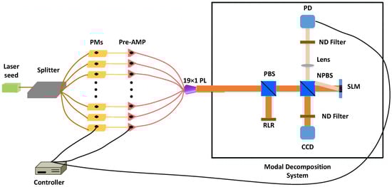
Figure 1.
Schematic diagram of a switchable output mode adaptive control system based on a 19 × 1 photonic lantern. The mode decomposition system is based on the optical correlation filter method [33]. Key components include PMs (phase modulators), Pre-AMP (pre-amplifier), PL (photonic lantern), PBS (polarizing beam splitter), NPBS (non-polarizing beam splitter), RLR (residual light receiver), ND (neutral density filter), SLM (spatial light modulator), CCD (near-field camera), and PD (photodetector).
Although we employed a mode decomposition system based on the optical correlation filter method, we did not perform a complete mode decomposition of the output intensity pattern. Instead, we only collected the power data for the desired modes. Therefore, in principle, the method of simply measuring the transmission matrix of the system and applying a straightforward matrix inversion for control would not work. The speed of the mode decomposition system based on the optical correlation method mainly depends on the frame rate of the far-field camera. In this work, we replaced the far-field camera with a photodetector. For commercial PDs, bandwidths exceeding 10 MHz can be readily achieved, thus significantly increasing the system’s speed. In the experimental system, we designed a controller driven by an FPGA, which can achieve speeds of over 100 MHz. This system allows for frame rates exceeding 10 MHz, enabling it to correct for disturbances occurring at kHz frequencies.
The SPGD algorithm augmented with basin hopping is selected for adaptive control because of the SPGD algorithm’s advantages, including rapid convergence, strong scalability, and high tolerance to power fluctuations. Despite these benefits, the SPGD algorithm can easily become trapped in local optima. The basin hopping algorithm mitigates this issue by facilitating the escape from local optima and enhancing the search for the global optimum. By combining the SPGD algorithm with the basin hopping algorithm, the system can achieve both rapid convergence and robust global optimization. To better comprehend the optimization process outlined in the provided content, a detailed flowchart is illustrated explaining the adaptive control procedure for optimizing voltages applied to a phase modulator and pre-amplifier, as seen in Figure 2. This flowchart can be divided into two primary sections: the SPGD algorithm and the basin hopping algorithm. Initially, the SPGD algorithm is utilized to quickly identify a local optimum. Starting voltages are defined and outputted to the phase modulator and pre-amplifier, followed by evaluating the initial performance function . The chosen method utilizes random disturbance voltages following a binomial distribution for each m-th iteration, which are added to the previous input voltages both positively and negatively, where the upper indices of represent phase modulators and pre-amplifiers, respectively. Subsequently, forward and backward evaluation functions and are obtained, providing critical gradient information for updating the modulation voltage iteratively as , where represents the gain coefficient. This process continues until either the maximum iteration number is attained or the objective function converges. Once a local optimum is identified, the basin hopping algorithm is utilized to continue the search for the global optimum. The acceptance criteria involve comparing the new evaluation function with the current local evaluation function . If , the new configuration is accepted and updates the solution. Otherwise, it is accepted with a probability adhering to the Metropolis criterion. The optimization concludes either after reaching the maximum iteration count or when no further improvement is observed, resulting in the final optimized voltage settings for the system.
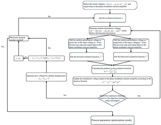
Figure 2.
Schematic flowchart depicting the procedure for executing mode control in an adaptive optics system that uses the SPGD + basin hopping algorithm.
3. Results and Discussion
3.1. Design and Performance Simulation of Photonic Lanterns
The proposed photonic lantern is schematically depicted in Figure 3. Specifically, Figure 3a provides a cross-sectional view of the single-mode end of the PL. In this figure, the numbers indicate the indices of the SMFs, which are arranged in a three-layer circularly symmetric configuration. When designing photonic lanterns, it is crucial to arrange the SMFs as compactly as possible to ensure efficient coupling of light fields, and the geometric arrangement of the SMF cores should match the modal structure supported by the multimode end because theoretical studies have shown that matching these structures can effectively reduce device loss. Following these design principles, the optimal configuration for a 19 × 1 photonic lantern is arranged in a three-layer circularly symmetric configuration: the innermost layer contains 1 SMF, the middle layer contains 6 SMFs, and the outermost layer contains 12 SMFs, ensuring efficient light coupling and minimizing losses by matching the modal structures between the single-mode and multimode ends. The parameters exploited in the design and simulation of this 19 ×1 photonic lantern are shown in Table 1. The core diameters of the single-mode fibers are 8 µm, and these fibers are arranged in a three-layer circular configuration forming a bundle having a diameter of 150 µm, which is surrounded by a low-refractive-index jacket. Based on our preliminary research, we found that the core-to-cladding ratio of the input single-mode fibers is a critical factor influencing mode evolution results in photonic lanterns. The results show that a larger core-to-cladding ratio can lead to purer mode output. To achieve better output beam quality, photonic lanterns with larger output core diameters require larger core-to-cladding ratios of the SMFs. Therefore, in designing this photonic lantern, we selected commercially available single-mode fibers having the largest core-to-cladding ratio (8/80) and corroded their cladding diameter to 30 µm, rather than using the commonly employed 10/125 single-mode fibers.
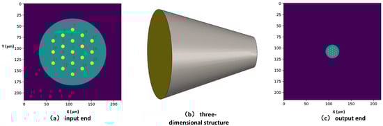
Figure 3.
Schematic diagram of 19 × 1 photonic lantern. The schematic representation of a 19 × 1 photonic lantern is depicted as follows: (a) the input end cross-section of the photonic lantern, (b) its three-dimensional structure, and (c) the output end cross-section of the photonic lantern. The serial numbers of the single-mode fibers are indicated in (a).

Table 1.
Physical parameters exploited in the design and simulation of this 19 × 1 photonic lantern.
The single-mode fiber bundle undergoes linear adiabatic tapering to form a gradually tapered transition zone, having a length of 3 cm, where the tapering ratio is 1:5. The taper ratio and taper length have an effect on the output performance of such a photonic lantern. The taper ratio directly determines the core diameter of the multimode output end of the photonic lantern and thus determines the number of modes that the output end can support. As the taper diameter gradually becomes finer, the single-mode fiber bundle turns into the core of a multimode fiber, while the jacket becomes the cladding of the multimode fiber. An excessively large taper ratio would result in the multimode output end supporting more than 19 modes, which would require more input arms to control the output modes. On the other hand, an overly small taper ratio would lead to the multimode output end supporting fewer than 19 modes. Taking the above into account, a taper ratio of 1:5 is a suitable value. While the taper length affects energy loss during the process of mode coupling, adiabatic transition requires that the change in the transverse dimensions of the single-mode fiber bundle within the tapering region must occur sufficiently slowly. This ensures that the mode coupling is minimized and energy loss is reduced during the transition process. A taper region that is too short fails to satisfy the adiabatic approximation, causing some light to leak out of the photonic lantern and increasing its loss. Conversely, a longer taper region ensures excellent mode coupling and low loss but increases fabrication difficulty. Considering both the insertion loss and the practical constraints of the manufacturing process, a taper length of 3 cm is deemed appropriate. The output end is spliced to a multi-mode fiber with dimensions and numerical aperture (NA = 0.095) matched to ensure optimal performance. Nineteen distinct modes can be supported by the multi-mode fiber, matching the number of input arms at the input end, which are LP01, LP02, LP03, LP11e, LP11o, LP12e, LP12o, LP21e, LP21o, LP22e, LP22o, LP31e, LP31o, LP32e, LP32o, LP41e, LP41o, LP51e, and LP51o, respectively.
As the taper diameter decreases, the confined optical fields within the single-mode fibers progressively converge and merge into supermodes. Figure 4 depicts the transformation process of the photonic lantern, starting from the input end where individual single-mode fibers propagate light independently, to the output end where these fields coalesce into the fundamental mode of a multi-mode fiber. At the initial stage, due to the relatively large spacing between the cores of the single-mode fibers, the optical fields propagate separately within each fiber. As the single-mode fibers taper down, they can no longer confine the optical fields, leading to leakage and gradual merging of the light fields. Although the Gaussian beam is circularly symmetric, the input configuration of the photonic lantern does not exhibit this symmetry. Instead, it shows symmetry, as evident in Figure 5. The amplitude decreases from the center outward, following a Gaussian-like distribution of the fundamental mode. The amplitude and phase differences among the single-mode fiber bundles in the second layer are relatively minor, while those in the third layer are more significant, which can be observed from the transmission matrix in the Supplementary Material File S1.
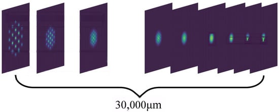
Figure 4.
The evolution to the fundamental mode in the 19 × 1 photonic lantern.
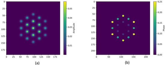
Figure 5.
Amplitude (a) and phase (b) of the light field at the single-mode input end generating into the fundamental mode of multi-mode fiber.
The amplitude at the single-mode input end of the photonic lantern, which can output the other 18 high-order LP modes, is illustrated in Figure 6. One can observe that the light intensity at the single-mode input end shares some similarities with the distribution of the corresponding high-order mode fields. However, there are also notable differences in the distribution patterns. Furthermore, when comparing the same o and e degenerate states, the input end lacks 90° symmetry. This is due to the fact that the o and e degenerate states have symmetry, while the photonic lantern structure has symmetry.
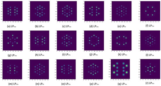
Figure 6.
Amplitude of the single-mode input end for the evolution into the other 18 high-order LP modes in the 19 × 1 photonic lantern.
These observations highlight the complex interplay between the input field distribution and the modal properties of the photonic lantern. Insertion loss (IL) is a critical parameter for characterizing the photonic lantern’s ability to output the desired modes. Before calculating the insertion loss for various output modes of the photonic lantern, it is first necessary to obtain its transmission matrix. Using this matrix, the required optical parameters (amplitudes and phases) at the input arms for generating the corresponding output modes can be deduced. The detailed steps are as follows: first, inject laser light individually into each single-mode (SM) input port. Next, perform mode decomposition at the multimode (MM) output port to measure the normalized mode decomposition coefficients for each SM input. Using these coefficients, construct the transmission matrix M of the photonic lantern, which is
Once the transmission matrix M is determined, apply the corresponding input vectors by injecting laser light with the appropriate intensity and phase differences into the SM input ports. For example, to generate the fundamental mode at the output, the input power for each SM fiber should be proportional to the square of the modulus of the corresponding element in the first row of the transmission matrix M, and the phase difference should match the phase of the corresponding element in the first row. Finally, measure the total output power at the MMF output port to validate the performance. , where is the power of the corresponding output mode, and is the power at each input arm. Since this work focuses on the design and simulation of a 19 × 1 photonic lantern, the calculated insertion losses represent ideal conditions. These losses only account for the leakage of the optical field during the mode evolution process. Other practical losses, such as Fresnel reflection losses introduced during the actual fabrication process, have not been considered in these calculations.
This photonic lantern demonstrates high-efficiency output of LP modes, as evidenced by the insertion efficiencies listed in Table 2. Overall, all the modes exhibit insertion efficiencies exceeding 98%, with a trend indicating that higher-order modes (corresponding to lower effective refractive indices) tend to have slightly lower efficiencies. Specifically, the lowest insertion efficiency observed is 98.43% for the mode, equating to an insertion loss of approximately 0.07 dB. In summary, the photonic lantern achieves excellent performance across various modes, ensuring minimal signal loss even for higher-order modes, despite the noted symmetry differences.
Table 2.
Insertion efficiency of different LP modes.
A phase vortex beam carrying orbital angular momentum can be generated by the linear superposition of the two degenerate states of the mode (where ) with equal amplitudes and a phase difference of . Therefore, the photonic lantern can similarly evolve efficiently and effectively into OAM modes. As illustrated in Figure 7, which uses the mode as an example, the photonic lantern transitions from a single-mode input to a phase vortex beam within the taper region. Similar to the evolution of the fundamental mode, at the initial stage, the beams are tightly confined within the cores of the SMFs due to their large core-to-core distances, propagating independently. As the taper diameter decreases, the beams begin to leak out of the SMFs and gradually merge. By the output end, the beams have fully coalesced, forming a new core from the SMF bundle, with the jacket serving as the new cladding. The beams ultimately evolve into the eigenmode of a new multi-mode fiber.
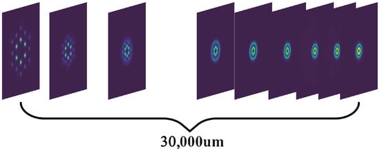
Figure 7.
The evolution of the mode in the 19 × 1 photonic lantern.
Given that OAM modes are hollow beams, the intensity at the center SMF (SMF-0) is nearly zero. Although the OAM beam’s intensity distribution is circularly symmetric, the intensity distribution at the single-mode input end lacks this symmetry. This is due to the fact that OAM modes carry orbital angular momentum, leading to asymmetric inputs among SMFs at the same layer. These properties can be understood through the transmission matrix of the OAM modes, as detailed in Supplementary Materials File S2. Given that this multimode fiber supports 16 LP high-order modes (with ), it is capable of generating a total of 16 OAM modes. Figure 8 shows the 16 OAM modes that can be generated by the photonic lantern. The orientation of the arrows signifies the rotational direction of the beam (clockwise or counterclockwise), whereas the number of arrows represents the absolute value of the topological charge l. As shown in the figure, the photonic lantern can output ultra-pure OAM modes. Given that the 19 × 1 photonic lantern efficiently outputs modes (where ), and OAM modes are coherent superpositions of these modes, the photonic lantern can also efficiently generate OAM modes. The transmission efficiency of these OAM modes falls between the efficiencies of the and modes (where ).
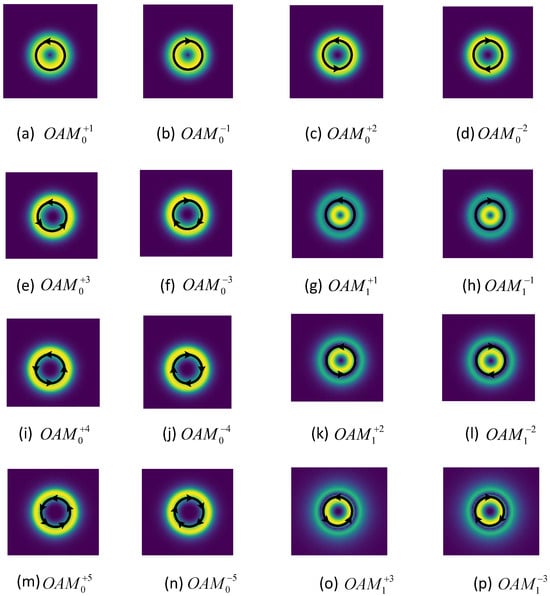
Figure 8.
The 19 OAM modes that can be generated by the PL. The direction of the arrows indicates the rotation direction of the beam (clockwise or counterclockwise), while the number of arrows represents the absolute value of the topological charge l.
A good design is fundamental to achieving high-quality photonic lanterns, but precise fabrication is equally critical for their performance. Although the fabrication and control of the 19 × 1 photonic lantern are not the primary focus of this study, we can briefly introduce some of the most critical aspects of the design process.
Cleanliness: Cleanliness of both the optical fibers and the glass tubes is crucial throughout the entire process. Any dirt or liquid residue can cause intense burning during the fusion and tapering stages, significantly reducing the yield. Even tiny contaminants can become the primary source of loss in the final photonic lantern.
Bundling Techniques: Precise control over the inner diameter of the pre-tapered glass sleeve is essential to ensure that the fiber bundle is tightly and uniformly arranged. Custom molds may be required to achieve specific geometric arrangements, ensuring optimal packing density and alignment.
Fusion Tapering Parameters: The choice of flame size and tapering speed during the fusion process affects the collapse effect, which alters the size of air holes between single-mode fibers or determines whether the glass sleeve and fiber bundle shrink proportionally. Ensuring proportional shrinking is critical for the success of the splicing step. Therefore, selecting appropriate fusion tapering parameters is vital for achieving high-quality results.
3.2. Mode Adaptive Output Control Based on the 19 × 1 Photonic Lantern
Although, as previously mentioned, photonic lanterns can achieve efficient and high-purity mode outputs, this goal is challenging to attain in practical applications. The primary reasons are the following. Firstly, it is difficult to precisely control the amplitude and phase parameters of the input arms of the photonic lantern; secondly, minor environmental disturbances can alter the optical parameters of the input arms, leading to instability in the output modal field. Environmental disturbances, such as air flow and base vibrations causing fiber jitter, can affect the amplitudes and phases of the input arms of the PL. The fiber output is highly sensitive to these disturbances, impacting signal stability. Additionally, instabilities in optical components, such as laser seeds and splitters, also contribute to these perturbations. Our preliminary measurements in the laboratory indicate that phase jitter occurs at frequencies ranging from approximately 1 kHz to 10 kHz, while amplitude jitter occurs at frequencies ranging from about 1 Hz to 10 Hz. To simulate these disturbances, we modeled all jitter as a combination of a 10 kHz random phase jitter and a 10 Hz random amplitude jitter applied to the input arms of the photonic lantern. In simulations, we modeled amplitude perturbations with a variation of up to 20% and phase perturbations with variations up to radians. The controller bandwidth was designed to be 10 MHz to effectively correct these environmental perturbations. Previously, we have implemented adaptive control systems for 3 × 1, 5 × 1, and 6 × 1 photonic lanterns [22,25,26,27,28,29]. On this basis, we will expand the control channels to 19 and introduce a high-speed mode decomposition system into the control system. In the previous work, we used PMs which are lithium niobate phase modulators with a 10 GHz bandwidth and control accuracy of 0.1 mrad, and a Pre-AMP with an output of the 10 W level and control accuracy in mW, whose precision has far exceeded the required control accuracy of .
In this simulation, the transmission matrix of the PL needs to be determined in advance because we rely on it to obtain the mode information at the multimode output of the PL. However, in actual experiments, it is not necessary to know the transmission matrix beforehand. The SPGD algorithm can adaptively search for the optimal solution as long as there is a one-to-one correspondence between the input and output, without requiring explicit knowledge of their specific relationship. During operation, the mode decomposition device is continuously required because perturbations are not static. Real-time adaptive control is necessary based on the results of mode decomposition to maintain optimal performance.
These difficulties are particularly pronounced for the 19 × 1 photonic lantern due to its higher control complexity. Therefore, an adaptive control system is essential to achieve stable, high-purity mode outputs. Here, we employ the SPGD algorithm augmented with basin hopping for adaptive control, the processes of which are detailed in Section 2.2. The phase and amplitude of the input arms are adjusted using the adaptive control algorithm, while polarization is controlled by a polarization controller to align the polarization direction consistently. Although the system appears linear in the optical field, directly inverting the PL transmission matrix combined with output mode measurements is challenging. Firstly, direct inversion of the PL transmission matrix requires high-speed and precise measurement of the amplitude and phase information at the input arms of the photonic lantern. Secondly, accurately obtaining the transmission matrix of a photonic lantern is extremely difficult due to manufacturing defects, which cause the actual transmission matrix to deviate from the designed one. Lastly, in high-power applications, we typically connect a fiber amplifier after the photonic lantern. Mode decomposition for control is performed after the amplifier, where the SPGD adaptive control algorithm can also account for mode competition within the fiber amplifier. Given these challenges, the SPGD combined with the basin hopping algorithm is a more suitable control strategy for managing the modes in photonic lanterns.
The fundamental mode of fiber lasers, owing to its superior beam quality and high energy concentration, has found widespread application in various fields, such as the industrial and medical sectors. Therefore, we first applied this control system to achieve stable, high-purity fundamental mode control through simulation. Figure 9a illustrates the mode content evolution and the final output beam generated by the 19 × 1 photonic lantern during the adaptive control process, specifically targeting the fundamental mode output. Figure 9b shows how the M2 value varies with process time for the fundamental mode. These figures clearly demonstrate that the application of the active control algorithm results in a gradual increase in the fundamental mode content and a progressive decrease in the M2 factor. Ultimately, the output fundamental mode content surpasses 99%, achieving an M2 value better than 1.07, indicating excellent beam quality.
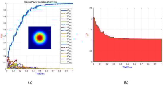
Figure 9.
Control effect of the output fundamental mode. (a) Mode content evolution and the final output beam generated by the 19 × 1 photonic lantern during the adaptive control process, targeting the fundamental mode output. (b) The value as a function of process time during the adaptive control process.
For high-order LP modes, we selected the LP21e mode as an example to study the mode control process and its control effect. Figure 10 illustrates the mode content evolution and the final output beam generated by the 19 × 1 photonic lantern during the adaptive control process, with the objective of achieving LP21e mode output. At the outset, environmental disturbances cause the optical parameters of the photonic lantern’s input arms to deviate from their optimal settings. As a result, the output beam contains a substantial number of unwanted modes, leading to a highly disordered beam profile. This initial state underscores the necessity of adaptive control mechanisms to stabilize and optimize the output. Through the adaptive control algorithm, the system effectively adjusts the phase and amplitude of the input arms, thereby producing the desired high-purity mode stably. The final output achieves a purity of over 95% for the LP21e mode. This result demonstrates the effectiveness of the proposed adaptive control strategy in managing high-order mode transitions. By dynamically adjusting the phase and amplitude of the input arms, the system successfully stabilizes the desired mode, even in the presence of environmental disturbances. The key to effective control lies in the ability to quickly find the global optimum rather than getting trapped in a local optimum. Here, we present simulation results using only the SPGD algorithm, as shown in Figure 11. The results indicate that the controlled output of the LP21e mode content reached only 72%, which is significantly lower compared to the >95% mode content achieved in Figure 10. This discrepancy is due to the SPGD algorithm converging to a local optimum rather than the global solution.
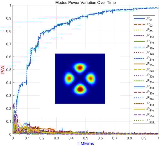
Figure 10.
Mode content evolution and the final output beam generated by the 19 × 1 photonic lantern during the adaptive control process, targeting LP21e mode output.
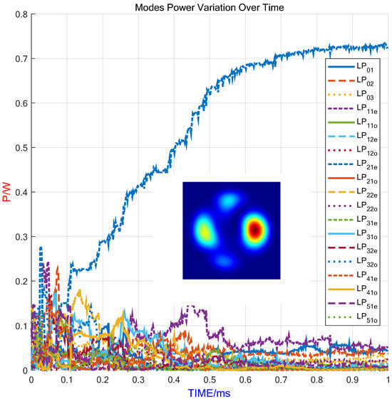
Figure 11.
Mode content evolution and the final output beam generated by the 19 × 1 photonic lantern using only the SPGD algorithm, targeting LP21e mode output.
Figure 12 and Figure 13 illustrate the generation of the additional 18 LP modes and 16 OAM modes by the 19 × 1 photonic lantern within the adaptive control system. As evident from the figures, the LP and OAM modes generated by the adaptive control system show a high degree of similarity to their corresponding standard mode field patterns. This close resemblance indicates that the generated modes possess a high level of purity. Table 3 presents the final output mode purity of the target modes obtained from this simulation. From the table, it is evident that for all controlled modes, the final output mode purity is ≥90%. Despite the inherent randomness in each simulation run, the results consistently show that the output modes maintain a purity exceeding 90%. Additionally, it is observed that the purity of lower-order modes is generally higher compared to that of higher-order modes. This suggests that lower-order modes are more easily controlled and maintained at higher purities. The results highlight the system’s capability to produce stable and high-fidelity modes, even under varying environmental conditions. In summary, the adaptive control system effectively ensures the generation of high-purity LP and OAM modes, validating its practical utility in advanced optical applications.
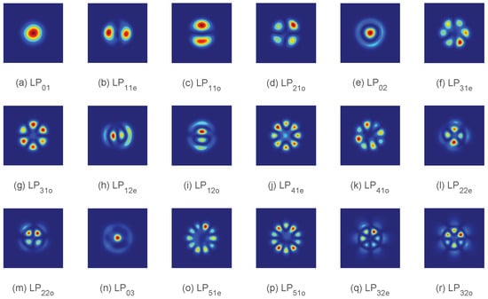
Figure 12.
The other 18 LP modes generated by the 19 × 1 photonic lantern in the adaptive control system.
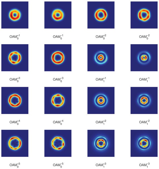
Figure 13.
The 16 OAM modes generated by the 19 × 1 photonic lantern in the adaptive control system.
Table 3.
The mode purity of generation for the 19 LP modes and 16 OAM modes by the 19 × 1 photonic lantern within the adaptive control system.
In our previous simulations using a 19 × 1 photonic lantern with an adaptive control system, we achieved dynamic switching between 19 LP modes and 16 OAM modes, ensuring high-quality output with over 90% mode purity. However, despite these promising simulation results, the actual fabricated photonic lanterns still exhibit differences from their simulated counterparts. During the fused tapering process of PLs, factors such as flame stability, uniformity of flame temperature, and taper speed stability can lead to discrepancies between the actual fabricated PLs and simulated PLs. These inconsistencies primarily manifest in two ways: (1) transmission matrix mismatch; (2) increased insertion loss. The transmission matrix mismatch does not affect control performance, as the SPGD algorithm can adaptively search for the optimal solution as long as there is a one-to-one correspondence between the input and output, without requiring explicit knowledge of their specific relationship, while for increased insertion loss, it exacerbates the thermal effect, which leads to reduced mode coupling efficiency and changes in modal field shape. To mitigate the thermal effect, first, select PLs with low insertion loss, and second, place the PLs in a water-cooled environment to minimize the adverse effects caused by thermal effects. Through these improvements, we aim to achieve a robust and highly efficient experimental setup that closely matches the theoretical predictions, thereby validating the feasibility of our proposed approach.
4. Conclusions
In this study, we have successfully designed and simulated a 19 × 1 photonic lantern capable of efficiently outputting 19 LP modes and 16 OAM modes with minimal insertion loss not exceeding 0.07 dB. Utilizing the beam propagation method, we meticulously analyzed the mode evolution process and insertion loss, deriving the transmission matrix for our photonic lantern design. The simulation results indicate that our device can evolve into various high-order modes with remarkable efficiency, demonstrating the potential to significantly enhance the performance of optical systems in applications such as optical communication, imaging, and particle manipulation. Furthermore, by integrating an adaptive control system incorporating mode decomposition and employing the SPGD plus basin hopping algorithm, we achieved dynamic switching between different modes, ensuring high-quality output with over 90% mode purity.
Our research highlights the significant potential of photonic lanterns in addressing the challenges associated with generating and controlling multiple high-order modes within fiber-based systems. By enabling precise and efficient conversion from single-mode inputs to the desired high-order modes, our proposed 19 × 1 photonic lantern opens new avenues for enhancing the functionality and versatility of optical devices. Specifically, the capability to dynamically adjust and optimize the output modes in real time offers substantial advantages in managing TMI and improving signal quality in high-power applications. Moreover, the successful demonstration of OAM mode generation using our photonic lantern underscores its applicability across a broader spectrum of optical technologies, including those requiring beams with orbital angular momentum.
Despite these advancements, further research is necessary to overcome the existing limitations and improve the overall performance of photonic lanterns. Key areas for future investigation include reducing insertion losses, enhancing mode purity, and increasing robustness against environmental fluctuations. Additionally, exploring new structural designs and fabrication could lead to more compact and efficient photonic lanterns, expanding their range of applications. In summary, this work contributes to the development of advanced multi-mode fiber systems using photonic lantern technology, providing useful insights for their application in special fields.
Supplementary Materials
The following supporting information can be downloaded at https://www.mdpi.com/article/10.3390/photonics12090911/s1; File S1: Transmission matrix of the LP modes; File S2: Transmission matrix of the OAM modes.
Author Contributions
Conceptualization, W.L., Y.Y. and P.L.; methodology, Y.Z., H.Z., B.Y., Q.Z. and D.Z.; writing—review and editing P.L. and W.L. All authors have read and agreed to the published version of the manuscript.
Funding
This research was funded by National Natural Science Foundation of China, grant number 12204540.
Data Availability Statement
The original contributions presented in this study are included in the article/Supplementary Material. Further inquiries can be directed to the corresponding authors.
Conflicts of Interest
The authors declare no conflicts of interest.
References
- Ramachandran, S.; Fini, J.M.; Mermelstein, M.; Nicholson, J.W.; Ghalmi, S.; Yan, M.F. Ultra-large effective area higher order mode fibers: A new strategy for high power laser. Laser Photonics Rev. 2008, 2, 429–448. [Google Scholar] [CrossRef]
- Fini, J.M.; Ramachandran, S. Natural bend-distortion immunity of high-order-mode large-mode-area fibers. Opt. Lett. 2007, 32, 748–750. [Google Scholar] [CrossRef] [PubMed]
- Newkirk, A.V.; Antonio-Lopez, J.E.; Velazquez-Benitez, A.; Albert, J.; Amezcua-Correa, R.; Schülzgen, A. Bending sensor combining multicore fiber with a mode-selective photonic lantern. Opt. Lett. 2015, 40, 5188–5191. [Google Scholar] [CrossRef]
- Chelkowsko, S.; Hild, S.; Freise, A. Prospects of higher-order Laguerre-Gauss modes in future gravitational wave detectors. Phys. Rev. D Part. Fields Gravit. Cosmol. 2009, 79, 122002. [Google Scholar] [CrossRef]
- Noack, A.; Bogan, C.; Willke, B. Higher-order Laguerre-Gauss modes in (non-) planar four-mirror cavities for future gravitational wave detectors. Opt. Lett. 2017, 42, 751–754. [Google Scholar] [CrossRef]
- Chang, W.; Feng, M.; Mao, B.; Wang, P.; Wang, Z.; Liu, Y.-G. All-fiber fourth-order OAM mode generation employing a long period fiber grating written by preset twist. J. Light. Technol. 2022, 40, 4804. [Google Scholar] [CrossRef]
- Mo, S.; Zhu, H.; Liu, J.; Liu, J.; Zhang, J.; Shen, L.; Wang, X.; Wang, D.; Li, Z.; Yu, S. Few-mode optical fiber with a simple double-layer core supporting the O + C + L band weakly coupled mode-division multiplexing transmission. Opt. Express 2023, 31, 2467–2479. [Google Scholar] [CrossRef]
- Velázquez-Benítez, A.M.; Guerra-Santillán, K.Y.; Caudillo-Viurquez, R.; Antonio-López, J.E.; Amezcua-Correa, R.; Hernández-Cordero, J. Optical trapping and micromanipulation with a photonic lantern-mode multiplexer. Opt. Lett. 2018, 43, 1303–1306. [Google Scholar] [CrossRef]
- Liu, J.; Zhang, J.; Liu, J.; Lin, Z.; Li, Z.; Lin, Z.; Zhang, J.; Huang, C.; Mo, S.; Shen, L.; et al. 1-Pbps orbital angular momentum fiber-optic transmission. Light Sci. Appl. 2022, 11, 202. [Google Scholar] [CrossRef]
- Fang, J.; Li, J.; Kong, A.; Xie, Y.; Lin, C.; Xie, Z.; Lei, T.; Yuan, X. Optical orbital angular momentum multiplexing communication via inversely-designed multiphase plane light conversion. Photonics Res. 2022, 10, 2015–2023. [Google Scholar] [CrossRef]
- Lin, K.H.; Kuan, W.H. Ultrabroadhand long-period fiber gratings for wavelength-tunable doughnut beam generation. IEEE Photon. Technol. Lett. 2023, 35, 203–206. [Google Scholar] [CrossRef]
- Ma, C.; Wang, D.; Deng, H.; Yuan, L. Stable orbital angular momentum mode generator based on helical long-period fiber grating. Opt. Fiber Technol. 2022, 73, 103019. [Google Scholar] [CrossRef]
- Zhang, K.; Wu, P.; Dong, J.; Du, D.; Yang, Z.; Xu, C.; Guan, H.; Lu, H.; Qiu, W.; Yu, J.; et al. Broadband mode-selective couplers based on tapered side-polished fibers. Opt. Express 2013, 29, 19690–19702. [Google Scholar] [CrossRef]
- Ngcobo, S.; Litvin, I.; Burger, L.; Forbes, A. A digital laser for on-demand laser modes. Nat. Commun. 2013, 4, 2289. [Google Scholar] [CrossRef]
- Eznaveh, Z.S.; Zacarias, J.C.; Lopez, J.E.; Shi, K.; Milione, G.; Jung, Y.; Thomsen, B.C.; Richardson, D.J.; Fontaine, N.; Leon-Saval, S.G.; et al. Photonic lantern broadhand orbital angular momentum mode multiplexer. Opt. Express 2018, 26, 30042–30051. [Google Scholar] [CrossRef] [PubMed]
- Birks, T.A.; Gris-Sánchez, I.; Yerolatsitis, S.; Leon-Saval, S.G.; Thomson, R.R. The photonic lantern. Adv. Opt. Photonics 2015, 7, 107–167. [Google Scholar] [CrossRef]
- Chen, S.Y.; Liu, Y.G.; Wang, Z.; Guo, H.; Zhang, H.; Mao, B. Mode transmission analysis method for photonic lantern based on FEM and local coupled mode theory. Opt. Experss 2020, 28, 30489–30501. [Google Scholar] [CrossRef] [PubMed]
- Chen, L.; Guo, H.; Shi, Z.; Chang, W.; Chen, B.; Wang, Z.; Liu, Y. Low-loss, high-purity, and ultrabroadband all-fiber LP41 mode converter employing a mode-selective photonic lantern. Chin. Opt. Lett. 2023, 21, 110008. [Google Scholar] [CrossRef]
- Zhao, L.; Li, W.; Chen, Y.; Yu, T.; Zhao, E.; Tang, J. Design and characterization of a self-matching photonic lantern for all few-mode fiber laser systems. Opt. Experss 2024, 32, 16799–16808. [Google Scholar] [CrossRef]
- Lopez-Galmiche, G.; Eznaveh, Z.S.; Antonio-Lopez, J.E.; Velazquez-Benitez, A.M.; Rodriguez-Asomoza, J.; Herrera-Piad, L.A.; Sanchez-Mondragon, J.J.; Gonent, C.; Sillard, P.; Li, G.; et al. Gain-controlled erbium-doped amplifier using mode selective photonic lantern. In Next-Generation Optical Communication: Components, Sub-Systems, and Systems V, Proceedings of the SPIE OPTO, San Francisco, CA, USA, 13–18 February 2016; SPIE: Bellingham, WA, USA, 2016; Volume 9774, p. 97740P. [Google Scholar] [CrossRef]
- Lopez-Galmiche, G.; Eznaveh, Z.S.; Antonio-Lopez, J.E.; Velazquez Benitez, A.M.; Rodriguez Asomoza, J.; Sanchez Mondragon, J.J.; Gonnet, C.; Sillard, P.; Li, G.; Schülzgen, A.; et al. Few-mode erbium-doped fiber amplifier with photonic lantern for pump spatial mode control. Opt. Lett. 2016, 41, 2588–2591. [Google Scholar] [CrossRef]
- Lu, Y.; Chen, Z.; Liu, W.; Jiang, M.; Yang, J.; Zhou, Q.; Zhang, J.; Chai, J.; Jiang, Z. Stable single transverse mode excitation in 50 µm core fiber using a photonic-lantern-based adaptive control system. Optics Express 2022, 30, 22435–22441. [Google Scholar] [CrossRef]
- Montoya, J.; Aleshire, C.; Hwang, C.; Fontaine, N.K.; Velázquez-Benítez, A.; Martz, D.H.; Fan, T.Y.; Ripin, D. Photonic lantern adaptive spatial mode control in LMA fiber amplifiers. Opt. Experss 2016, 24, 3405–3413. [Google Scholar] [CrossRef]
- Montoya, J.; Hwang, C.; Martz, D.; Aleshire, C.; Fan, T.Y.; Ripin, D.J. Photonic lantern kw-class fiber amplifier. Opt. Experss 2017, 25, 27543–27550. [Google Scholar] [CrossRef] [PubMed]
- Lu, Y.; Jiang, Z.; Chen, Z.; Jiang, M.; Yang, J.; Zhou, Q.; Zhang, J.; Zhang, D.; Chai, J.; Yang, H.; et al. High-power orbital angular momentum beam generation using adaptive control system based on mode selective photonic lantern. J. Light. Technol. 2023, 41, 5607–5613. [Google Scholar] [CrossRef]
- Zhou, Q.; Lu, Y.; Li, C.; Chai, J.; Zhang, D.; Liu, P.; Zhang, J.; Jiang, Z.; Liu, W. Transmission matrix-inspired optimization for mode control in a 6×1 photonic lantern-based fiber laser. Photonics 2023, 10, 390. [Google Scholar] [CrossRef]
- Lu, Y.; Liu, W.; Chen, Z.; Jiang, M.; Zhou, Q.; Zhang, J.; Li, C.; Chai, J.; Jiang, Z. Spatial mode control based on photonic lanterns. Opt. Express 2021, 29, 41788–41797. [Google Scholar] [CrossRef]
- Ze, Y.; Liu, P.; Zhang, H.; Hu, Y.; Ding, L.; Yan, B.; Zhang, J.; Zhou, Q.; Liu, W. Realizing a kilowatt-level fiber amplifier with a 42 µm core diameter fiber for improved multi-mode performance towards single mode operation output through adaptive spatial mode control utilizing a 3 × 1 photonic lantern. Opt. Express 2024, 32, 35794–35805. [Google Scholar] [CrossRef]
- Ze, Y.X.; Liu, P.F.; Zhang, H.W.; Hu, Y.; Ding, L.; Yan, B.; Zhang, J.; Zhou, Q.; Liu, W. The simulation of mode control for a photonic lantern adaptive amplifier. Micromachines 2024, 15, 1342. [Google Scholar] [CrossRef]
- Bhattacharya, D.; Sharma, A. Finite difference split step method for non-paraxial semivectorial beam propagation in 3D. Opt. Quant. Electron. 2008, 40, 933–942. [Google Scholar] [CrossRef]
- Shibayama, J.; Matsubara, K.; Sekiguchi, M.; Yamauchi, J.; Nakano, H. Efficient nonuniform schemes for paraxial and wide-angle finite-difference beam propagation methods. J. Light. Technol. 1999, 17, 677–683. [Google Scholar] [CrossRef]
- Lin, J.W. Lightbeam: Simulate Light Through Weakly-Guiding Waveguides. Astrophysics Source Code Library. 2020. Available online: https://ui.adsabs.harvard.edu/abs/2021ascl.soft02006L/abstract (accessed on 10 September 2025).
- Chai, J.Y.; Liu, W.G.; Wang, X.L.; Zhou, Q.; Xie, K.; Wen, Y.; Zhang, J.; Liu, P.; Zhang, H.; Zhang, D.; et al. High-speed modal analysis of dynamic modal coupling in fiber oscillator. Front. Phys. 2023, 11, 1146208. [Google Scholar] [CrossRef]


Disclaimer/Publisher’s Note: The statements, opinions and data contained in all publications are solely those of the individual author(s) and contributor(s) and not of MDPI and/or the editor(s). MDPI and/or the editor(s) disclaim responsibility for any injury to people or property resulting from any ideas, methods, instructions or products referred to in the content. |
© 2025 by the authors. Licensee MDPI, Basel, Switzerland. This article is an open access article distributed under the terms and conditions of the Creative Commons Attribution (CC BY) license (https://creativecommons.org/licenses/by/4.0/).