Abstract
This paper proposes an intelligent power adaptation framework for Free-Space Optics (FSO) communication systems operating under different weather conditions exploiting a deep learning (DL) analysis of received eye diagram images. The system incorporates two Convolutional Neural Network (CNN) architectures, LeNet and Wide Residual Network (Wide ResNet) algorithms to perform regression tasks that predict received signal quality metrics such as the Quality Factor (Q-factor) and Bit Error Rate (BER) from the received eye diagram. These models are evaluated using Mean Squared Error (MSE) and the coefficient of determination ( score) to assess prediction accuracy. Additionally, a custom CNN-based classifier is trained to determine whether the BER reading from the eye diagram exceeds a critical threshold of ; this classifier achieves an overall accuracy of 99%, correctly detecting 194/195 “acceptable” and 4/5 “unacceptable” instances. Based on the predicted signal quality, the framework activates a dual-amplifier configuration comprising a pre-channel amplifier with a maximum gain of 25 dB and a post-channel amplifier with a maximum gain of 10 dB. The total gain of the amplifiers is adjusted to support the operation of the FSO system under all-weather conditions. The FSO system uses a 15 dBm laser source at 1550 nm. The DL models are tested on both internal and external datasets to validate their generalization capability. The results show that the regression models achieve strong predictive performance, and the classifier reliably detects degraded signal conditions, enabling the real-time gain control of the amplifiers to achieve the quality of transmission. The proposed solution supports robust FSO communication under challenging atmospheric conditions including dry snow, making it suitable for deployment in regions like Northern Europe, Canada, and Northern Japan.
1. Introduction
Over the past several decades, mobile communication systems have undergone a rapid evolution, with each generation emerging roughly every ten years since the introduction of first-generation (1G) networks in the 1980s. The allocated carrier frequency spectrum of 1G to fourth-generation (4G) technologies has primarily ranged from 700 MHz to 2.6 GHz [1]. However, the limited bandwidth within this range, coupled with the exponential increase in mobile device penetration and global data traffic, has resulted in persistent challenges related to spectrum congestion and capacity limitations. These issues have been further exacerbated by the advent of data-intensive applications enabled by emerging technologies such as fifth- and sixth-generation (5G and 6G) networks, the Internet of Things (IoT), smart urban infrastructure, and cloud-based platforms.
The growing demand for high-throughput, low-latency, and reliable communication services has placed a significant strain on existing Radio Frequency (RF) resources, which are increasingly constrained by spectral scarcity and interference. In response to these challenges, FSO communication has attracted considerable interest as a promising complementary solution.
FSO systems offer several key advantages, including fiber-comparable data rates, rapid and cost-effective deployment, unlicensed access to a wide optical frequency band, and enhanced physical layer security [2,3]. FSO communication has demonstrated versatility across a wide range of applications, including inter-building links, healthcare services, defense systems, and various other domains [4]. Despite its promising capabilities, FSO technology remains highly sensitive to environmental factors. Specifically, its performance can be significantly affected by atmospheric disturbances and adverse weather conditions such as scintillation, fog, haze, rainfall, and snow, as well as misalignment-induced pointing errors between the optical transmitter and receiver [5]. These impairments contribute to signal attenuation and result in transmission power losses that can severely degrade the reliability and overall efficiency of the FSO communication link. FSO systems use narrow beams within the Near-Infrared (NIR) range to establish Line-of-Sight (LoS) communication. The 1550 nm wavelength is commonly preferred for its low atmospheric attenuation and superior receiver sensitivity [5,6]. While FSO systems inherently provide high data rates and low latency owing to their direct LoS transmission, the increasing complexity of optical network infrastructures presents challenges in accurately assessing signal quality [7]. These challenges stem from dynamic network configurations and varying environmental conditions that affect link performance. Recent advances in optical signal measurement and analysis have introduced effective tools for comprehensive performance monitoring, facilitating the more reliable management of optical links across diverse operational scenarios [8]. The eye diagram serves as a fundamental tool for evaluating signal quality within optical communication systems. It encapsulates essential information about the optical signal’s behavior alongside other system-related parameters. Notably, visual data such as eye diagrams offer meaningful insights into the condition and performance of the signal. Despite being static in nature, these eye diagram visualizations effectively illustrate the system’s response under defined operating conditions. They have been widely utilized to assess signal integrity and to characterize various impairments commonly encountered in Intensity Modulation–Direct Detection (IM-DD)-based optical systems [9].
Traditional methods for analyzing eye diagrams typically depend on expert interpretation, which can introduce human error and increase operational overhead. To mitigate these limitations, machine learning (ML) algorithms have been increasingly adopted in optical communication systems for automated signal quality assessment [10]. The use of ML algorithms in optical communication systems offers the benefit of delivering rapid and precise performance metrics, which can be integrated into feedback control mechanisms to dynamically adjust system parameters such as filter settings, electronic dispersion compensation and power adjustments. ML algorithms can infer the system’s operating condition, enabling autonomous decisions such as rerouting data across alternative network paths or initiating retransmission without requiring human intervention. Additionally, traditional ML algorithms for eye diagram analysis have undergone a major shift with the emergence of deep learning (DL) techniques. Unlike conventional ML algorithms, which often lack the capability to support efficient end-to-end learning, deep learning models offer significantly enhanced learning capacity. Deep Neural Networks (DNNs) characterized by multiple nonlinear layers and a large number of interconnected neurons utilizing activation functions form the backbone allow this advancement. Various deep learning architectures such as Convolutional Neural Networks (CNNs), Recurrent Neural Networks (RNNs), and Deep Reinforcement Learning (DRL) have demonstrated remarkable success across numerous domains including image processing, natural language understanding, and autonomous systems [11].
Future optical networks are expected to be highly adaptive and support various modulation formats to accommodate increasing data demands. However, their heterogeneous nature introduces diverse transmission impairments, making real-time Optical Performance Monitoring (OPM) metrics like the Bit Error Rate (BER), Quality Factor (Q-factor), and transmission distance an essential requirement at intermediate nodes for reliable signal quality assessment [12].
1.1. Related Work
There are several studies that have used a CNN algorithm in optical communications. In [13], a CNN-based decoding method was proposed for differential FSO systems using bipolar complementary pulse width modulation (BCPWM), which improves signal amplitude and reduces common-mode interference. The model operates without channel state information by directly analyzing the received signals. The results showed that the CNN outperforms BNRZ, ML, and Volterra detectors, achieving lower SNR requirements for a target BER of . The study focused solely on symbol-level signal demodulation using CNNs and required raw received signal waveforms as input. This approach does not address practical scenarios where direct signal access is limited or where only eye diagrams are available for performance monitoring. Additionally, the work lacks an investigation related to estimating key physical-layer performance metrics such as the BER and Q-factor, which are crucial for real-time optical system assessment and control. These gaps highlight the need for more adaptable CNN-based models that can extract meaningful performance insights from visual signal representations like eye diagrams without relying on prior channel knowledge.
In [14], a custom CNN model was designed and experimentally validated to classify On–Off Keying (OOK) bit sequences under varying Signal-to-Noise Ratios (SNRs), simulating thermal noise and atmospheric turbulence conditions. The study employs two CNNs: the first detects whether a given signal segment contains bit information, while the second classifies detected bits as logical ‘1′ or ‘0′. This two-stage approach helped reduce computational complexity during demodulation. The study demonstrated the effectiveness of CNNs in supporting high-throughput optical communication in noisy environments, offering reliable bit classification without imposing significant constraints on the size, weight, and power of the FSO setup. However, a key limitation of this approach is its reliance on controlled experimental conditions, which may not fully capture real-world turbulence dynamics. Additionally, the need for training separate networks adds system complexity and may introduce latency in real-time applications, especially under rapidly varying channel conditions.
The study in [15] used an end-to-end deep learning-based FSO communication system employing OOK modulation, demonstrating its ability to significantly reduce the BER without relying on channel state information (CSI). While effective, such systems often face challenges when dealing with dynamic or unpredictable channel variations that can degrade when the inference conditions deviate from the training scenarios. In contrast, the approach adopted in this study focuses on using CNNs, LeNet, and Wide ResNet to directly evaluate the BER and Q-factor from eye diagram images, which are widely recognized as visual indicators of signal integrity. This approach not only circumvents the need for explicit CSI but also leverages standard physical-layer diagnostic tools in optical networks. Furthermore, using eye diagrams as input allows for more generalized feature extraction, enabling robust performance monitoring across varying conditions without retraining for each specific channel model.
The work in [16] introduced a Deep Transfer Learning (TL) framework for a comprehensive analysis and diagnosis of eye diagrams in Optical Fiber Communication (OFC) systems. It employed a CNN algorithm to estimate fiber link lengths and extract essential eye diagram parameters such as the Q-factor, eye height, and eye width. By reusing learned features from a source task (e.g., estimating link length) for multiple target tasks (e.g., parameter estimation and impairment classification), the method achieved high accuracy and significantly reduced training times. While the results were good, the scope of the study was primarily limited to impairments caused by device imperfections and signal degradation in guided media. In contrast, the proposed study addresses eye diagram-based signal quality estimation in FSO communication systems, where the signal is susceptible to fundamentally different challenges such as atmospheric attenuation, atmospheric turbulence, beam misalignment, and weather-induced attenuation. These impairments require specialized learning models that can accommodate the stochastic and dynamic nature of FSO channels, representing a distinct research challenge not covered in OFC systems.
Additionally, the paper in [17] introduced a deep learning-driven approach for Q-factor prediction in OFC systems, employing CNN architectures such as LeNet, Wide ResNet, and Inception-v4. These models were trained on eye diagrams corresponding to OOK and level four Pulse-Amplitude Modulation (PAM4 formats). Similarly, the study did not address the unpredictable-prone environment of FSO links. In contrast, our study targets eye diagram analysis in FSO systems, where deep learning models must contend with atmospheric effects and more volatile channel conditions, introducing a fundamentally different set of challenges.
In [18], the authors tackled the complex issue of optimal power distribution for wavelength division multiplexing (WDM)-based radio over FSO (RoFSO) systems by introducing two adaptive algorithms guided by channel state information (CSI). Initially, they proposed a model-driven Stochastic Dual Gradient (SDG) approach that offers exact solutions but requires accurate system modeling and reliable CSI estimation. To address these dependencies, a second, model-independent method was developed, namely, the Primal–Dual Deep Learning (PDDL) algorithm. This approach employs deep neural networks to learn the optimal power allocation strategy by simultaneously updating primal and dual variables, without needing explicit knowledge of the system or channel model. A policy gradient technique is used to compute the learning updates. The simulation results demonstrated that both proposed techniques significantly outperform traditional equal power allocation schemes. The model-free PDDL method, in particular, shows strong potential for broader deployment in FSO systems, where modeling complexity and turbulence estimation remain major challenges.
In [19], an embedded power allocation framework was proposed for optical wireless communication systems operating over various fading environments, including foggy conditions, Rayleigh and Rician fading, and the Gamma–Gamma turbulence model. This system facilitates real-time power optimization under noisy and fluctuating channel conditions, helping to enhance transmission speed and minimize signal interference. Notably, the solution demonstrated high accuracy levels reaching approximately 99% in Rician fading channels, 97% in standard and Rayleigh scenarios, and 96% in fog-affected environments. Additionally, it achieved maximum data rates of 2.8 Gbps for binary phase shift keying (BPSK), 5.6 Gbps for quadrature phase shift keying (QPSK), 11.2 Gbps for 16 level quadrature amplitude modulation (16 QAM), and 16.81 Gbps for 64 QAM.
In [20], the problem of optical power allocation was investigated under both power budget and eye safety constraints for adaptive WDM-based FSO transmission systems. The study aimed to mitigate the impact of weather-induced turbulence on signal quality and system performance. For conventional systems, a basic water-filling algorithm was proposed to distribute power across multiple wavelengths. However, for WDM RoFSO systems, a dedicated power allocation algorithm was developed, demonstrating superior capacity and robustness. The results showed that this method could maintain high data rates even over long distances or under challenging weather conditions.
Several studies have explored the application of deep learning models, particularly CNNs, for extracting critical features from eye diagrams to estimate key performance parameters such as the Q-factor and bit error rate in optical communication systems. While these models have shown promise, their effectiveness in terms of computational efficiency, robustness, and extraction accuracy remains an open area of research. These issues become even more significant in FSO communication systems, which are highly susceptible to harsh environmental conditions like heavy fog and dry snow. In such dynamic and challenging scenarios, ensuring reliable and adaptive performance monitoring is vital to maintaining link stability and data integrity.
1.2. Contribution
This work introduces an intelligent signal quality estimation and power adaptation framework for FSO communication systems using machine learning models applied to eye diagram analysis. The primary objective is to enhance signal integrity and link reliability under adverse weather conditions, particularly in harsh snow-prone environments. The key contributions of this work are as follows:
- ∘
- Intelligent signal quality prediction from eye diagrams: We develop and train lightweight CNN architectures, including LeNet and Wide ResNet, to accurately predict the Q-factor or the BER directly from eye diagram images. This regression-based prediction enables the fine-grained assessment of optical signal quality under varying channel impairments.
- ∘
- Classification-based reliability decision using CNNs: In parallel, we design a binary classifier CNN that determines whether the BER exceeds a critical threshold of , providing a rapid decision-making mechanism for triggering signal retransmission with adaptive power control.
- ∘
- Dual-model power adaptation strategy: Based on the outputs of the prediction or classification model, a dual-amplifier configuration is selectively activated. When the predicted BER exceeds the threshold, the system engages a pre-channel booster amplifier (maximum gain 25 dB) and a post-channel preamplifier (maximum gain 10 dB) to maintain robust communication over a 0.6 km FSO link in harsh environments.
- ∘
- Validation under harsh weather conditions: The proposed system is evaluated under simulated dry snow conditions to emulate the signal degradation typically encountered in cold regions such as Northern Europe, Canada, and Northern Japan. The experimental results demonstrate the effectiveness of the proposed models in maintaining acceptable signal quality.
- ∘
- Comprehensive performance evaluation: The LeNet and Wide ResNet regression models are evaluated using training and validation loss curves along with the mean square error (MSE) and score to ensure convergence and generalization. The CNN classifier is assessed using confusion matrices, precision, recall, and the F1-score, providing a thorough evaluation of classification performance.
- ∘
- Generalizability across datasets: All developed models are further tested using eye diagram samples from an external dataset, confirming their generalization capability and robustness to dataset variability.
The rest of the paper is organized as follows. Section 2 presents the design of the CNN classifier, LeNet-based regression model, and Wide ResNet-based regression model. Section 3 describes the proposed intelligent power adaptation framework employing DL models within the FSO communication system. Section 4 provides the simulation results along with a detailed analysis and discussion. Finally, Section 5 concludes the paper with a summary of the key findings.
2. CNN Algorithms
A variety of convolutional neural network (CNN) architectures have been implemented and are extensively utilized in deep learning, particularly for image classification and computer vision applications. In this study, we consider a regular CNN for classification, LeNet for regression, and Wide ResNet for regression.
2.1. CNN Model
CNNs represent a specialized class of Artificial Neural Networks (ANN) optimized for extracting meaningful features from data arranged in grid formats, such as images and videos. Their capability to effectively identify spatial hierarchies makes them highly applicable in visual data analysis, especially within computer vision domains. A typical CNN architecture is composed of several layers, including an input layer, convolutional layers, pooling layers, etc. All layers are shown in Figure 1.
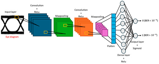
Figure 1.
CNN architecture used for classification.
Each layer plays a distinct role in processing and transforming the input data to extract relevant features for the learning task. In this study, we used a CNN for classification among different BER readings extracted from eye diagrams above or below the set value.
2.2. LeNet Model
LeNet is a pioneering CNN architecture developed by Yann LeCun and colleagues at AT&T Bell Labs in the late 1980s. It was initially developed for recognizing handwritten digits. LeNet represents a structured method for feature extraction, incorporating two convolution layers followed by average pooling and fully connected layers, concluding with a SoftMax output [10].
In this study, we utilize the LeNet architecture to predict the values of the BER and Q-factor. Figure 2 illustrates a schematic diagram of the LeNet model designed for regression tasks.
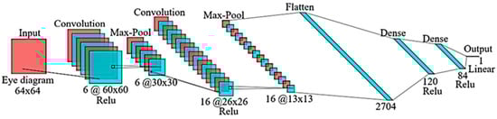
Figure 2.
CNN architecture used for regression.
The model consists of nine layers: an input layer, two convolutional layers, two max-pooling layers, a flatten layer, two dense layers, and an output layer. Initially, the eye diagram is pre-processed and resized to 64 × 64 pixels before being passed to the input layer. The first convolutional layer applies 6 filters of size 5 × 5, while the second convolutional layer uses 16 filters, also of size 5 × 5. The Relu activation function is applied in both convolutional layers. Each convolutional layer is followed by a max-pooling layer with a pool size of 2 × 2, which reduces the spatial dimensions. After the second max-pooling operation, the output is flattened into a one-dimensional vector and passed through two fully connected dense layers. The first dense layer contains 120 neurons, and the second contains 84 neurons. Both layers employing Relu activation. Finally, the output layer consists of a single neuron with a linear activation function, which outputs either the BER or the Q-factor, depending on the specific prediction target.
2.3. Wide ResNet Model
The Wide ResNet model addresses the vanishing gradient problem inherent in deep neural architecture. It introduces a broadened layer structure integrated with residual connections, enhancing gradient flow during training [16]. Figure 3 depicts the architecture of the implemented Wide ResNet architecture that is used for regression in this study.
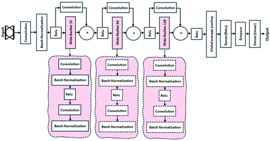
Figure 3.
Wide ResNet architecture used for regression.
The model is designed for regression tasks and consists of multiple key components: an input layer, an initial convolutional block, three wide residual blocks, a global average pooling layer, a dense layer, a dropout layer, and an output layer. The input images are pre-processed and resized to dimensions of 64 × 64 × 1, then passed through a convolutional layer with 16 filters of size 3 × 3, followed by batch normalization and a Relu activation function. Next, the feature maps are sequentially processed through three wide residual blocks with increasing filter sizes of 32, 64, and 128, respectively. Each residual block contains two convolutional layers with 3 × 3 filters, batch normalization, and Relu activations along with a shortcut connection that adjusts the dimensions when necessary. After the residual learning process, a global average pooling operation reduces each feature map to a single value, minimizing overfitting and computational complexity. The output is then passed through a dense layer with 128 Relu-activated units, followed by a dropout layer with a 50% dropout rate to prevent overfitting. Finally, the output layer contains a single neuron with a linear activation function and L1–L2 regularization, producing a continuous-valued output such as the predicted Q-factor.
3. Design of Proposed Intelligent FSO System
Figure 4 presents the structural layout of the IM-DD FSO transmission system, developed using OptiSystem 22.1 in conjunction with Python version 3.11.4. The proposed setup is employed to evaluate the performance of the proposed eye diagram analysis technique based on deep learning.
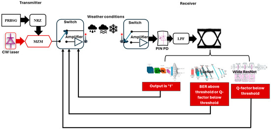
Figure 4.
Layout of proposed intelligent FSO system.
We investigated a 10 Gbps FSO communication system that adopts an On–Off Keying (OOK) modulation scheme. OOK is widely recognized for its applicability in data center interconnect environments due to its simplicity and reduced implementation cost. Compared to more complex modulation formats such as Quadrature Amplitude Modulation (QAM), OOK provides a practical balance between performance and system complexity, making it well suited for high-speed and energy-efficient optical transmission in cost-sensitive applications.
3.1. Transmitter Module
At the transmitter module, a 10 Gbps electrical signal is encoded on a bit stream produced by a Pseudo-Random Bit Sequence Generator (PRBSG) and modulated by an optical carrier generated from continuous wave (CW) laser operating at 1550 nm via a Mach-Zehnder Modulator (MZM), which facilitates high-speed modulation while preserving signal integrity and enabling reliable optical data transmission. Real-time feedback from the received eye diagram, a switching mechanism in the project, is employed to dynamically choose between transmission with or without optical amplification. A booster optical amplifier with a maximum gain of 25 dB is activated if any of the following conditions are met: the classified BER value is larger than , the BER predicted from the eye diagram using LeNet is larger than , or the Q-factor predicted from the eye diagram using either LeNet (for first dataset) or Wide ResNet (for the second dataset) is below the specified threshold. The amplification setup adopts a dual-stage configuration, comprising a pre-channel optical amplifier with a maximum gain of 25 dB and a post-channel amplifier offering up to 10 dB gain. This adaptive approach enhances transmission reliability by dynamically adjusting the gain in the system to accommodate the fluctuation of atmospheric conditions. Additionally, after the signal is transmitted using the selected amplifier configuration, the receiver monitors the actual BER of the received signal in real time. If this measured BER exceeds the predefined threshold, the system infers that the initial prediction may have been based on a suboptimal or corrupted eye diagram input. In such cases, the system can either request retransmission with an adjusted amplifier configuration or prompt the re-capture of the eye diagram for reanalysis. This feedback pathway ensures that the system adapts dynamically to unforeseen signal degradation and maintains the desired quality of service.
The operational logic of the switching mechanism is summarized in Algorithm 1.
| Algorithm 1. Adaptive Optical Amplifier Selection Based on Eye Diagram Analysis | |
| Input) | |
| Output: Amplifier configuration decision | |
| 1: | Initialize: |
| 2: | Define BER and Q-factor thresholds as: |
| and | |
| 3: | Acquire eye diagram: |
| Capture the received eye diagram from the receiver. | |
| 4: | Valid input: |
| Check if eye diagram is valid | |
| If invalid: | |
| Request re-acquisition or apply error-handling procedure | |
| Return to step 3 | |
| 5: | Predict performance metrics: |
| a. For BER: | |
| Classification of BER CNN (eye diagram) Predicted BER LeNet (eye diagram dataset1) | |
| b. For Q-factor | |
| Predicted BER LeNet (eye diagram dataset1) Predicted BER Wide ResNet (eye diagram dataset2) | |
| 6: | Evaluate conditions: |
| 7: | If any of the following conditions are satisfied: |
| ) | |
| Predicted BER > | |
| 8: | Then |
| Select dual-stage amplification | |
| -Pre-channel amplifier: Max. gain = 25 dB | |
| -Post-channel amplifier: Max. gain = 10 dB | |
| 9: | Else: |
| Transmit without amplification | |
| 10: | Configure transmission: |
| Apply the selected amplifier configuration | |
| 11: | Transmit signal |
| Launch the modulated optical signal through the FSO channel | |
| 12: | Collect feedback: |
| Measure actual BER and Q-factor after transmission | |
| 13: | Adjust amplification based on feedback |
| If actual BER > or actual Q-factor < : | |
| Increase amplifier gain or initiate retransmission | |
| Else: | |
| Transmit without amplification | |
| 14: | Return: |
| Amplifier settings used during the current transmission session | |
3.2. FSO Channel
The modulated optical signal is subsequently transmitted through the FSO channel. The proposed framework is adaptable to various atmospheric conditions, including haze, fog, rain, snow, and cloud cover. In this particular investigation, the focus is placed on dry snow and cloud scenarios, aligning with deployment in regions frequently affected by snowfall. The impact of snow-induced attenuation on FSO performance is analyzed by distinguishing between two types of snowfall: dry snow and wet snow. The received optical power of an LoS FSO link is expressed as [21]
where is the received optical power, denotes the transmitted power, and and represent the transmitter and receiver optical efficiencies, respectively. The transmitter and receiver aperture diameters are donated by and , respectively. The beam divergence angle is represented by and denotes the propagation range in the FSO channel. Finally, the atmospheric weather attenuation is denoted by and its value depends on the weather condition. Table 1 shows the calculation of for foggy, rainy, and snowy weather conditions.

Table 1.
Attenuation of various weather conditions.
3.3. Receiver Module
At the receiver, the optical signal is processed according to the process described in Algorithm 1. In scenarios where the dual-amplifier arrangement is selected, the signal is initially amplified by a secondary optical amplifier with a gain of 10 dB prior to signal detection. The signal is directly routed to a positive–intrinsic–negative (PIN) photodetector (PD), where optical-to-electrical conversion is performed. The electrical signal obtained from the PD is passed through an Electrical Low-Pass Filter (ELPF) to suppress high-frequency components and mitigate out-of-band noise. Following the detection, a BER analyzer processes the filtered signal to evaluate the system performance by analyzing the corresponding eye diagram using three different deep learning (DL) models: CNN, LeNet, and Wide ResNet. The output of these models is subsequently used to control the switching mechanism as described in Algorithm 1 to determine whether the received signal should be forwarded to the end users or retransmitted with signal power amplification.
Algorithm 2 presents the used CNN-based model designed for the binary classification of the BER of the received signal using eye diagram images. The model takes a pre-processed black-and-white-scale eye diagram as input parameter, then it outputs a binary label indicating whether the BER exceeds a predefined threshold, leveraging a lightweight CNN architecture optimized for accurate and efficient BER discrimination.
| Algorithm 2. CNN for binary BER classification | |
| Input (grayscale) | |
| Output, where if BER , else | |
| 1: | Procedure ) |
| 2: | //Preprocessing |
| 3: | Normalize pixel values of to range |
| 4: | to shape (256, 192, 1) for CNN compatibility |
| 5: | //CNN Architecture Definition |
| 6: | with the following layers |
| 7: | Input Layer: shape (256, 192, 1) |
| 8: | Conv2D Layer 1: 32 filters, kernel size (3 × 3), activation = Relu |
| 9: | MaxPooling2D Layer 1: pool size (2 × 2) |
| 10: | Conv2D Layer 2: 64 filters, kernel size (3 × 3), activation = Relu |
| 11: | MaxPooling2D Layer 2: pool size (2 × 2) |
| 12: | Flatten Layer |
| 13: | Dense Layer: 128 units, activation = Relu |
| 14: | Output Layer: Dense(1), activation = Sigmoid |
| 15: | //Model Training |
| 16: | using: |
| 17: | Loss function: Binary Cross-Entropy |
| 18: | Optimizer: Adam |
| 19: | (based on ) |
| 20: | //Inference |
| 21: | //Predict label from input image |
| 22: | Return: |
| 23: | End Procedure |
Algorithm 3 outlines an LeNet-based CNN framework for predicting continuous-valued signal quality metrics, such as the BER or Q-factor, from eye diagram images. The architecture is trained using MSE loss and leverages a compact convolutional structure to perform efficient and accurate regression.
| Algorithm 3. LeNet-Based Model for BER or Q-factor Prediction | |
| Input(black & white scale) | |
| Output, representing either BER or Q-factor | |
| 1: | Procedure ) |
| 2: | //Preprocessing |
| 3: | Resize input image to shape (64×64) |
| 4: | Normalize pixel values of to the range |
| 5: | (64, 64, 1) for LeNet input |
| 6: | //LeNet Architecture Definition |
| 7: | as follows: |
| 8: | Input Layer: shape (64, 64, 1) |
| 9: | Conv2D Layer 1: 6 filters, kernel size (5 × 5), activation = Relu |
| 10: | MaxPooling2D Layer 1: pool size (2 × 2) |
| 11: | Conv2D Layer 2: 16 filters, kernel size (5 × 5), activation = Relu |
| 12: | MaxPooling2D Layer 2: pool size (2 × 2) |
| 13: | Flatten Layer |
| 14: | Dense Layer 1: 120 units, activation = Relu |
| 15: | Dense Layer 2: 84 units, activation = Relu |
| 16: | Output Layer: Dense(1), linear activation (for regression output) |
| 17: | //Model Training |
| 18: | using: |
| 19: | Loss function: MSE |
| 20: | Optimizer: Adam |
| 21: | Target values: Continuous BER or Q-factor measurements |
| 22: | //Prediction |
| 23: | //Predict BER or Q-factor |
| 24: | Return: |
| 25: | End Procedure |
Algorithm 4 details a Wide ResNet regression model developed for Q-factor prediction from eye diagram images. The model consists of an initial convolutional layer followed by multiple wide residual blocks with increasing filter dimensions, global average pooling, and a fully connected regression head. The network is trained using MSE loss and it is validated with early stopping to optimize generalization performance.
| Algorithm 4. Wide ResNet for Q-prediction | |
| Input(grayscale) | |
| Output | |
| 1: | Procedure) |
| 2: | //Preprocessing |
| 3: | Resize input image to shape (64 × 64) |
| 4: | Normalize pixel values of to the range |
| 5: | (64, 64, 1) for LeNet input |
| 6: | //Define Wide Residual Block |
| 7: | Function WideResBlock(x, filters) |
| 8: | |
| 9: | Conv2D: filters, 3 × 3, stride = 1 |
| 10: | Relu |
| 11: | Conv2D: filters, 3 × 3, stride = 1 |
| 12: | BatchNorm |
| 13: | filters: |
| 14: | Conv2D: filters, 1 × 1, stride = 1 (for shortcut) |
| 15: | Element-wise Add: residual + shortcut |
| 16: | Relu |
| 17: | Return output |
| 18: | End Function |
| 19: | //Build Wide ResNet Architecture |
| 20: | as follows: |
| 21: | |
| 22: | Relu |
| 23: | WideResBlock with 32 filters |
| 24: | WideResBlock with 64 filters |
| 25: | WideResBlock with 128 filters |
| 26: | GlobalAveragePooling2D |
| 27: | Dense: 128 units, activation = Relu |
| 28: | Dropout: rate = 0.5 |
| 29: | Output Layer: Dense(1), linear activation (for regression output) |
| 30: | //Model Training |
| 31: | Split dataset into training and validation sets |
| 32: | with: |
| 33: | Loss function: MSE |
| 34: | Optimizer: Adam |
| 35: | Target values: Q-factor measurement |
| 36: | Train model with early stopping and validation loss monitoring |
| 37: | //Prediction |
| 38: | |
| 39: | Return: |
| 40: | End Procedure |
In this work, two datasets are constructed for training and evaluation purposes. The first dataset comprises 1000 black and white eye diagram images. The dataset is applied then to binary BER classification using a CNN model and BER/Q-factor regression using the LeNet architecture. The second dataset contains 5000 eye diagram frames and it is utilized exclusively for training the Wide ResNet model for Q-factor prediction. The larger dataset size for the Wide ResNet model is required due to its deeper and wider architecture, which generally necessitates a greater volume of training data to ensure robust generalization and to mitigate overfitting.
4. Simulation Results and Discussion
This section presents the evaluation outcomes of the proposed ML-driven power control framework of the proposed FSO communication system. The assessment is conducted under practical system settings, including a wavelength of 1550 nm, transmitter and receiver aperture diameters of 4 cm and 36 cm, respectively, optical efficiencies at both ends (), and a beam divergence angle of 2 mrad. In the case of heavy fog, heavy rain, wet snow, and dry snow, the values of are 85 dB/km (0.2 km visibility), 19.28 dB/km, 13.73 dB/km, and 96.8 dB/km, respectively [23,25].
The main objective of the proposed system is to ensure that the received signal at an FSO link of 0.6 km maintains a BER and Q-factor above their respective threshold values under all-weather conditions. If the received signal falls below these thresholds due to factors such as atmospheric attenuation or FSO channel losses, the system triggers signal retransmission using optical amplification to restore signal quality.
The eye diagram images used in both dataset 1 and dataset 2 are generated across various FSO link ranges and under diverse weather conditions, including heavy fog, heavy rain, wet snow, and dry snow. A CW laser source with an output power of 15 dBm is employed to simulate baseline signal degradation under these adverse atmospheric scenarios. Furthermore, each dataset of the eye diagram images is partitioned into 80% for training and 20% for testing to enable performance evaluation.
All simulations including the training and evaluation of the CNN, LeNet, and Wide ResNet models are conducted with a Windows 11 Home (64-bit) computer. The system was equipped with a 12th Generation Intel® Core™ i9-12900H processor (20 threads, base frequency ~2.5 GHz) and 32 GB of RAM.
The results are divided into four parts as follows.
4.1. Performance of FSO System Without Any Deep Learning Algorithms
Figure 5 illustrates the system performance over varying FSO link ranges under different atmospheric conditions, with subfigures (a) and (b) showing the Q-factor and BER, respectively. The analysis considers a minimum transmission distance of 0.6 km, with performance thresholds defined as a Q-factor of 4.07 and a BER of . It is clear that, in the absence of power adaptation, the received signal quality is insufficient under severe weather conditions such as heavy fog and dry snow. Specifically, at a free space distance of 0.6 km, the system exhibits a BER of 1 and a Q-factor of 0, underscoring its inability to maintain reliable communication under such adverse scenarios. Given that dry snow imposes the most severe degradation among the evaluated weather conditions, the following analyses are restricted to this scenario.
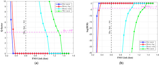
Figure 5.
System performance over varying FSO link ranges under different atmospheric conditions. (a) Q-factor and (b) BER.
Figure 6 shows the influence of optical amplifier gain on BER performance under dry snow conditions for an FSO link length of 0.6 km. Due to the substantial attenuation of 96.8 dB/km introduced by dry snow, achieving reliable signal detection necessitates considerable optical amplification. One can observe from Figure 6 that when the total gain remains below 33.3 dB, the system fails to meet the BER target, exhibiting BER = 1. In contrast, increasing the gain leads to a marked enhancement in BER performance, with an acceptable threshold attained at a gain level of 35 dB.
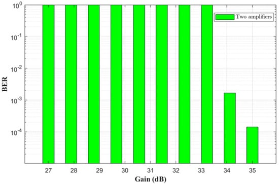
Figure 6.
BER versus overall gain of optical amplifiers.
This observation illustrates how amplifier gain is applied incrementally based on the severity of signal degradation, as inferred from the predicted BER or Q-factor. For example, using the full 25 dB from the pre-channel amplifier with only 1 dB from the post-channel amplifier does not suffice to meet the BER threshold. As additional gain is introduced from the second amplifier, the BER improves progressively. Full gain from both amplifiers (25 dB + 10 dB) is only applied when necessary to achieve acceptable signal quality. This approach avoids unnecessary power usage and ensures efficient and adaptive amplification in response to real-time channel conditions.
4.2. Performance Evaluation of CNN-Based BER Classifier
In this subsection, the results of using the CNN for BER classification will be discussed. Here, we used the first dataset. The model assigns a binary label to each input image, where a label of ‘1′ indicates that the corresponding BER is below the predefined threshold, and a label of ‘0′ denotes that it exceeds the threshold.
Figure 7 shows an accuracy plot for the proposed CNN classifier. One can notice that the model demonstrates robust generalization, as the accuracy curve rapidly converges within the early epochs and remains consistently high throughout the training phase.
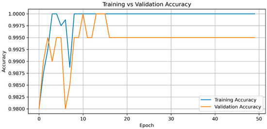
Figure 7.
Accuracy curve for BER CNN classifier model.
In the domain of computer vision, model evaluation is commonly conducted through a set of standardized performance indicators, including accuracy, precision, recall, and the F1-score. The corresponding mathematical expressions for these parameters are as following [26]:
where T, P, F, and N, denote true, positive, false, and negative, respectively.
Among these metrics, the accuracy remains a principal criterion, offering a comprehensive measure of the model’s predictive effectiveness and playing a central role in the overall assessment framework.
The confusion matrix presented in Figure 8 illustrates the classification performance of the proposed model in distinguishing eye diagram images based on a BER threshold of 10−4. The model successfully identified all 196 samples from the majority class (BER ≤ 10−4) with no false positives, demonstrating high specificity. For the minority class (BER > 10−4), the model correctly classified three out of four instances while misclassifying one instance as belonging to the majority class. These results reflect the model’s strong discriminatory capability, particularly for the dominant class, and its reasonable generalization to under-represent samples. The overall accuracy achieved is approximately 99.5%, indicating a high level of reliability for BER-based eye diagram classification.
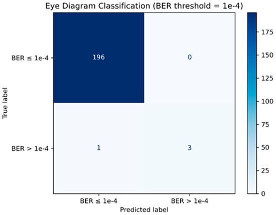
Figure 8.
Confusion matrix.
The trained BER CNN classifier model demonstrated strong classification performance in distinguishing between eye diagrams corresponding to low and high BER levels. Specifically, it correctly classified 194 out of 195 instances with a BER below the threshold and 4 out of 5 instances with the BER above the threshold, resulting in an overall accuracy of 99%. For the dominant class (BER ), the model achieved high precision, recall, and F1-score values near 0.99, indicating excellent reliability in identifying low-BER conditions. While the minority class (BER ) comprised a limited number of samples, the model still maintained a precision of 1.00 and an F1-score of 0.86, reflecting good generalization capability under class imbalance.
We took a sample eye diagram from another dataset that has a BER reading of and applied it to the model to be sure that the proposed BER CNN classifier model works properly. The model classifies it correctly as “1”, meaning the BER is above the threshold. Figure 9 illustrates the model’s classification confidence for a sample eye diagram using a horizontal bar chart. The chart displays the predicted probabilities for the two output classes, BER and BER , based on the model’s sigmoid output. In this case, the classifier assigns a high confidence score of 0.9962 to the BER class, indicating a strong likelihood that the input eye diagram corresponds to a high BER scenario. This type of visualization aids in interpreting the model’s output by illustrating not only the predicted class but also the associated confidence level. For applications such as FSO systems, where reliability is critical, having access to the model’s confidence can be as important as the classification outcome itself, particularly when decisions must be made under uncertain conditions.
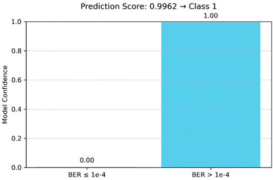
Figure 9.
The confidence visualization of the BER CNN classifier for a sample eye diagram image.
4.3. Performance Evaluation of LeNet-Based Model for BER and Q-Factor Prediction
In this section, the performance of the LeNet architecture is evaluated for predicting the Q-factor or BER from eye diagram inputs. The model is trained using first dataset of 1000 eye diagram images for 100 epochs. To rigorously assess its predictive capability and generalization performance, the Mean Squared Error (MSE) is employed as the primary evaluation metric. MSE quantifies the average squared difference between predicted and true Q-factor/BER values, providing a robust measure of the model’s overall prediction accuracy under diverse optical transmission conditions.
Figure 10 illustrates the MSE trends for the training and validation sets of the Q-factor (Figure 10a) and the BER (Figure 10b) over 100 epochs. The steep initial decline in MSE indicates the rapid learning of the underlying mapping between eye diagram features and the target quality metrics. Around epoch 40, both training and validation losses stabilize, suggesting convergence. The small gap between training and validation curves, coupled with a final validation MSE of 0.0757 (Q-factor) and 0.00049 (BER), reflects strong generalization. Moreover, the model achieves an score of 0.9688 for Q-factor prediction and 0.40 for BER prediction, underscoring its effectiveness and low risk of overfitting in practical FSO systems.
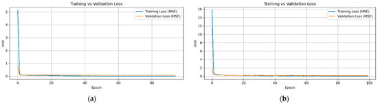
Figure 10.
MSE loss versus epoch for (a) Q-factor and (b) BER.
Figure 11 presents a comparison between the predicted and actual values for both the Q-factor and the BER. In Figure 11a, the predicted Q-factor values align closely with the diagonal reference line, indicating accurate regression performance. Similarly, Figure 11b shows strong agreement between the predicted and true BER values. These results confirm that the LeNet-based model can effectively approximate both performance metrics from eye diagram inputs.
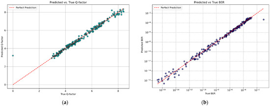
Figure 11.
Predicted versus true values using the LeNet model. (a) The Q-factor and (b) BER.
Table 2 illustrates a comparison between the predicted and actual Q-factor and BER values for eye diagram samples extracted from a different dataset acquired under amplification at a maximum transmission distance of 0.6 km under dry snow. This evaluation is intended to assess the generalization performance of the LeNet model under previously unseen conditions. The predicted Q-factor of 4.234272 demonstrates a minimal percentage error of approximately 0.101% relative to the true value of 4.230000, indicating highly precise regression performance. Similarly, for the BER, the predicted value of deviates from the true value of , yielding a percentage error of approximately 12.53%. These results confirm that the LeNet-based model maintains strong predictive accuracy for both performance metrics, even when applied to input conditions not encountered during training.
Table 2.
Comparison between true and predicted Q-factor and BER using LeNet-based regression model.
Finally, the system utilizes the predicted BER or Q-factor to make an informed decision regarding data retransmission with amplification. If the predicted BER exceeds a predefined threshold or the Q-factor falls below an acceptable level, this implies that the received signal quality is inadequate. Such degradation may arise from insufficient transmitter power, misalignment, or environmental impairments. In this case, optical amplification is employed to enhance signal reliability. Conversely, if the predicted BER is within acceptable limits and the Q-factor is sufficiently high, the data are considered successfully received and are forwarded to the end users without requiring retransmission.
4.4. Performance Evaluation of Wide ResNet-Based Model for Q-Factor Prediction
To evaluate the performance of the Wide ResNet architecture in regressing the Q-factor from eye diagram images, dataset 2 comprising 5000 frames is employed. This dataset is selected because Wide ResNet models typically require larger training sets than shallower architectures such as LeNet, due to their increased capacity and deeper hierarchical structure. The model is trained for up to 100 epochs with early stopping enabled, and convergence is achieved at epoch 49. The larger model capacity of Wide ResNet allows it to better extract abstract spatiotemporal features from complex eye diagrams, making it well suited for Q-factor prediction under varying transmission conditions. However, when applying the Wide ResNet architecture to predict BER values, the model did not generalize effectively. One possible reason for this limited performance is the small dynamic range and sparsity of BER values (ranges from to ), which can make it challenging for deep architectures to learn stable regression mappings without the use of specialized loss functions or value scaling strategies. Therefore, we did not consider the Wide ResNet algorithm for BER analysis and it was restricted to the Q-factor. Interestingly, a simpler LeNet model trained on a smaller dataset of only 1000 eye diagram frames demonstrated better generalization in BER prediction. This suggests that lightweight architecture may be more effective in scenarios where data distributions are narrow or heavily skewed.
Figure 12 demonstrates the training and validation MSE trajectories observed during the optimization of the Wide ResNet model on dataset 2. The early stages of training exhibit transient instability in validation error, which is characteristic of deeper models undergoing weight adaptation. This variability diminishes over time, and both curves gradually converge to low MSE values, indicating effective parameter learning and stable generalization. The minimal gap between training and validation losses in the later epochs reflects the benefit of architectural regularization strategies such as dropout and weight penalties and supports the model’s suitability for inferring Q-factor from high-dimensional visual input. The eventual convergence at epoch 49 suggests that, given enough samples, deeper convolutional architectures can achieve consistent performance in regression tasks involving complex signal representations. Moreover, the model attains an score of 0.9787 and a final MSE of 0.0555 for Q-factor prediction, demonstrating its high predictive accuracy and minimal overfitting risk in practical FSO communication systems.
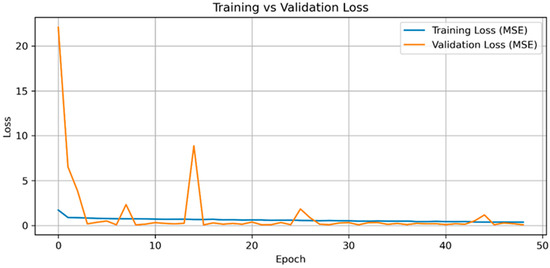
Figure 12.
Training and validation MSE curves for Wide ResNet-based Q-factor regression model.
Figure 13 displays the scatter plot of predicted versus actual Q-factor values on the validation set using the Wide ResNet model. The red dashed line represents the perfect prediction. The points are tightly clustered around this reference line across the full Q-factor range, indicating a strong linear correlation between predicted and ground-truth values.
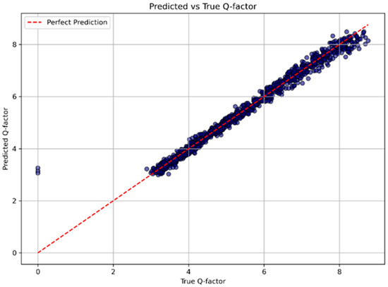
Figure 13.
Predicted versus true Q-factor values using the Wide ResNet model.
Additionally, to evaluate the generalization capability of the Wide ResNet model under previously unseen transmission conditions, a representative eye diagram image was selected from a separate dataset originally used for testing the LeNet model. As illustrated in Figure 14, the predicted and actual Q-factor values for this unseen sample exhibit a close match, with a relative error of approximately 0.95%.
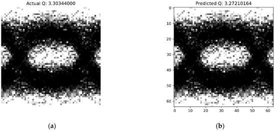
Figure 14.
Predicted versus true values of the Q-factor using the Wide ResNet model. (a) Actual and (b) predicted.
To evaluate the computational complexity and efficiency of the proposed Wide ResNet architecture, we measured the number of trainable parameters, floating-point operations (FLOPs), and average inference time per image, which are given in Table 3.
Table 3.
Wide ResNet model complexity and inference time.
Table 4 shows the summarized results obtained from the three CNN models that are used in this study. Classification accuracy and confusion breakdown are shown for the custom BER classifier. Regression models (LeNet and Wide ResNet) are evaluated using the MSE and score for Q-factor and BER prediction tasks.
Table 4.
Performance summary of various DL models.
4.5. Computation Complexity
Each model is trained and tested using black-and-white-scale image inputs with varying resolutions. Inference time was measured on a Windows 11 Home (64-bit) machine equipped with a 12th Gen Intel® Core™ i9-12900H processor and 32 GB RAM, using a CPU-only setup in a Jupyter Notebook version 7.3.2 environment. Table 5 summarizes the key complexity metrics.
Table 5.
Comparison between computation complexity for various DL models.
Although our proposed custom CNN BER classifier model presents a higher parameter count (5.42 million), larger memory footprint (20.70 MB), and longer inference time (0.1958 s) in comparison with benchmark models such as LeNet and Wide ResNet as observed in Table 5, it is important to note that these values were obtained under a CPU-only evaluation setup. In practical deployment scenarios, significant reductions in inference latency can be achieved through GPU acceleration or model optimization strategies such as quantization and pruning. Furthermore, the complexity of the proposed CNN is justified by the nature of its task: classifying whether the BER lies above or below a mission-critical threshold under noisy FSO conditions. This classification task necessitates finer feature extraction and the use of higher-resolution inputs (128 × 96), unlike the regression models that operate on coarser inputs (64 × 64) and predict a continuous BER value. Hence, the proposed model offers a necessary balance between accuracy and computational cost for reliable BER threshold detection in challenging optical environments.
Figure 15 illustrates the comparison of total parameters, memory footprint, and inference latency for the studied models. The LeNet architecture achieved a good balance between performance and efficiency, with relatively small parameter sizes and the lowest inference times. The Wide ResNet model demonstrated similar computational efficiency while maintaining model compactness due to its residual structure. The custom CNN, designed for classification, involved significantly more parameters and computation due to higher input resolution and deeper dense layers, making it more suitable for high-performance systems.
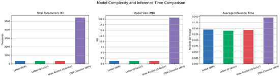
Figure 15.
Comparison between model complexity.
5. Conclusions
This work introduced a set of CNN models namely, LeNet, Wide ResNet, and a lightweight CNN classifier, for the intelligent assessment of signal quality for FSO systems. These models are used to determine whether the received signal meets predefined quality thresholds by predicting the BER or Q-factor, or by directly classifying the BER (from received eye diagrams), thereby enabling adaptive retransmission with power amplification strategies.
For the regression tasks, LeNet and Wide ResNet are used to predict BER and Q-factor values from eye diagram images. Their performance is evaluated using MSE and the score. LeNet, with 337k trainable parameters, achieved inference times of 0.1450 s and 0.1402 s per image for BER and Q-factor prediction, respectively. Wide ResNet, with 320k parameters and a complexity of 2.48 GFLOPs, achieved comparable accuracy with a slightly faster inference time of 82.63 ms/image. In the classification task, a CNN model is trained to categorize signal quality into “acceptable” or “unacceptable” based on a BER threshold. Model performance is evaluated using accuracy, confirming reliable decision-making capabilities under different channel conditions, and it achieves an accuracy of 99%.
To validate model generalizability, we tested all models on unseen eye diagram samples from a different dataset. The models successfully maintained strong performance across these external samples, demonstrating their robustness and practical applicability. Overall, the proposed approach provides a learning-based solution for real-time signal quality estimation. These models can be integrated into adaptive transmission frameworks to enhance the reliability of FSO systems.
Although the dataset used in this work was collected under weather-induced attenuation conditions, the proposed CNN-based models are applicable to any eye diagrams that reflect signal impairments whether due to atmospheric turbulence, attenuation, or pointing errors. Since eye diagrams encapsulate cumulative signal degradation, future work will explore the application of the proposed system to datasets generated under Gamma–Gamma and Log-Normal fading models, as well as channels with pointing error effects. While this study focuses on the BER and Q-factor as primary performance indicators, future work will extend the proposed framework to address adaptive throughput management to compensate for wavefront distortion, where real-time signal quality predictions can guide the selection of data rates or modulation schemes in FSO systems. This would enable dynamic performance optimization under varying atmospheric conditions
Author Contributions
Conceptualization, S.A.A.E.-M. and A.A.; methodology, S.A.A.E.-M. and A.A.; software, S.A.A.E.-M. and A.A.; validation, A.A.; formal analysis, S.A.A.E.-M. and A.A.; investigation, S.A.A.E.-M. and A.A.; resources, S.A.A.E.-M. and A.A.; writing—original draft preparation, S.A.A.E.-M.; writing—review and editing, A.A.; visualization, S.A.A.E.-M. and A.A.; funding acquisition, A.A. All authors have read and agreed to the published version of the manuscript.
Funding
This work received no funding.
Institution Review Board Statement
Not applicable.
Informed Consent Statement
Not applicable.
Data Availability Statement
The data are available upon request from the corresponding author.
Acknowledgments
This work is conducted under the High Throughput and Secure Networks Challenge Program at the National Research Council of Canada.
Conflicts of Interest
The authors declare no conflict of interest.
References
- Gilli, L.; Cossu, G.; Vincenti, N.; Bresciani, F.; Pifferi, E.; Schena, V.; Ciaramella, E. Intra-Satellite Optical Wireless Communications in Relevant Environments. In Proceedings of the 2023 23rd International Conference on Transparent Optical Networks (ICTON), Bucharest, Romania, 2–6 July 2023; pp. 1–4. [Google Scholar]
- Choudhary, A.; Agrawal, N.K. Inter-Satellite Optical Wireless Communication (IsOWC) Systems Challenges and Applications: A Comprehensive Review. J. Opt. Commun. 2022, 45, 925–935. [Google Scholar] [CrossRef]
- Khalighi, M.A.; Uysal, M.; Marseille, C.; Engineering, E. Survey on Free Space Optical Communication: A Communication Theory Perspective. IEEE Commun. Surv. Tutor. 2014, 16, 2231–2258. [Google Scholar] [CrossRef]
- Esmail, M.A.; Fathallah, H.; Alouini, M.-S. Outdoor FSO Communications Under Fog: Attenuation Modeling and Performance Evaluation. IEEE Photonics J. 2016, 8, 1–22. [Google Scholar] [CrossRef]
- Ahmed, H.Y.; Zeghid, M.; Khan, A.N.; Abd El-Mottaleb, S.A. Fuzzy Logic-Based Performance Enhancement of FSO Systems Under Adverse Weather Conditions. Photonics 2025, 12, 495. [Google Scholar] [CrossRef]
- Tanimura, T.; Hoshida, T.; Kato, T.; Watanabe, S.; Morikawa, H. Convolutional Neural Network-Based Optical Performance Monitoring for Optical Transport Networks. J. Opt. Commun. Netw. 2019, 11, A52–A59. [Google Scholar] [CrossRef]
- Zhang, W.; Zhu, D.; He, Z.; Zhang, N.; Zhang, X.; Zhang, H.; Li, Y. Identifying Modulation Formats through 2D Stokes Planes with Deep Neural Networks. Opt. Express 2018, 26, 23507. [Google Scholar] [CrossRef] [PubMed]
- Fan, X.; Xie, Y.; Ren, F.; Zhang, Y.; Huang, X.; Chen, W.; Zhangsun, T.; Wang, J. Joint Optical Performance Monitoring and Modulation Format/Bit-Rate Identification by CNN-Based Multi-Task Learning. IEEE Photonics J. 2018, 10, 1–12. [Google Scholar] [CrossRef]
- Xie, Y.; Wang, Y.; Kandeepan, S.; Wang, K. Machine Learning Applications for Short Reach Optical Communication. Photonics 2022, 9, 30. [Google Scholar] [CrossRef]
- Taye, M.M. Theoretical Understanding of Convolutional Neural Network: Concepts, Architectures, Applications, Future Directions. Computation 2023, 11, 52. [Google Scholar] [CrossRef]
- Pan, Z.; Yu, C.; Willner, A.E. Optical Performance Monitoring for the next Generation Optical Communication Networks. Opt. Fiber Technol. 2010, 16, 20–45. [Google Scholar] [CrossRef]
- Zheng, J.; Li, X.; Qiang, S.; Wang, Y. Decoding Scheme Based on CNN for Differential Free Space Optical Communication System. Opt. Commun. 2024, 559, 130449. [Google Scholar] [CrossRef]
- Bart, M.P.; Savino, N.J.; Regmi, P.; Cohen, L.; Safavi, H.; Shaw, H.C.; Lohani, S.; Searles, T.A.; Kirby, B.T.; Lee, H.; et al. Deep Learning for Enhanced Free-Space Optical Communications. Mach. Learn. Sci. Technol. 2023, 4, 045046. [Google Scholar] [CrossRef]
- Lohani, S.; Savino, N.J.; Glasser, R.T. Free-Space Optical ON-OFF Keying Communications with Deep Learning. In Proceedings of the Frontiers in Optics/Laser Science, Washington, DC, USA, 14–17 September 2020; p. FTh5E.4. [Google Scholar]
- Wang, D.; Xu, Y.; Li, J.; Zhang, M.; Li, J.; Qin, J.; Ju, C.; Zhang, Z.; Chen, X. Comprehensive Eye Diagram Analysis: A Transfer Learning Approach. IEEE Photonics J. 2019, 11, 1–19. [Google Scholar] [CrossRef]
- Cui, W.; Lu, Q.; Qureshi, A.M.; Li, W.; Wu, K. An Adaptive LeNet-5 Model for Anomaly Detection. Inf. Secur. J. A Glob. Perspect. 2021, 30, 19–29. [Google Scholar] [CrossRef]
- Sabri, A.A.; Hameed, S.M.; Hadi, W.A.H. Last Mile Access-Based FSO and VLC Systems. Appl. Opt. 2023, 62, 8402–8410. [Google Scholar] [CrossRef] [PubMed]
- Gao, Z.; Eisen, M.; Ribeiro, A. Optimal WDM Power Allocation via Deep Learning for Radio on Free Space Optics Systems. In Proceedings of the 2019 IEEE Global Communications Conference (GLOBECOM), Waikoloa, HI, USA, 9–13 December 2019; pp. 1–6. [Google Scholar]
- Akbari, M.; Olyaee, S.; Baghersalimi, G. Design and Implementation of Real-Time Optimal Power Allocation System with Neural Network in OFDM-Based Channel of Optical Wireless Communications. Electronics 2025, 14, 1580. [Google Scholar] [CrossRef]
- Zhou, H.; Mao, S.; Agrawal, P. Optical Power Allocation for Adaptive Transmissions in Wavelength-Division Multiplexing Free Space Optical Networks. Digit. Commun. Netw. 2015, 1, 171–180. [Google Scholar] [CrossRef]
- Kim, I.I.; McArthur, B.; Korevaar, E.J. Comparison of Laser Beam Propagation at 785 Nm and 1550 Nm in Fog and Haze for Optical Wireless Communications. In Optical Wireless Communications III; Korevaar, E.J., Ed.; SPIE: Ile-de-France, France, 2001; Volume 4214, pp. 26–37. [Google Scholar]
- Abd El-Mottaleb, S.A.; Singh, M.; Chehri, A.; Atieh, A.; Ahmed, H.Y.; Zeghid, M. Enabling High Capacity Flexible Optical Backhaul Data Transmission Using PDM-OAM Multiplexing. In Proceedings of the 2024 IEEE Global Communications Conference (GLOBECOM), Cape Town, South Africa, 8–12 December 2024; pp. 403–408. [Google Scholar]
- Muhammad, S.S.; Kohldorfer, P.; Leitgeb, E. Channel Modeling for Terrestrial Free Space Optical Links. In Proceedings of the 2005 7th International Conference Transparent Optical Networks, Barcelona, Spain, 7 July 2005; Volume 1, pp. 407–410. [Google Scholar]
- Nadeem, F.; Leitgeb, E.; Awan, M.S.; Kandus, G. Comparing the Snow Effects on Hybrid Network Using Optical Wireless and GHz Links. In Proceedings of the 2009 International Workshop on Satellite and Space Communications, Siena, Italy, 9–11 September 2009; pp. 171–175. [Google Scholar]
- Armghan, A.; Alsharari, M.; Aliqab, K.; Singh, M.; Abd El-Mottaleb, S.A. Performance Analysis of Hybrid PDM-SAC-OCDMA-Enabled FSO Transmission Using ZCC Codes. Appl. Sci. 2023, 13, 2860. [Google Scholar] [CrossRef]
- Mishra, N.K.; Singh, P.; Gupta, A.; Joshi, S.D. PP-CNN: Probabilistic Pooling CNN for Enhanced Image Classification. Neural Comput. Appl. 2024, 37, 4345–4361. [Google Scholar] [CrossRef]


Disclaimer/Publisher’s Note: The statements, opinions and data contained in all publications are solely those of the individual author(s) and contributor(s) and not of MDPI and/or the editor(s). MDPI and/or the editor(s) disclaim responsibility for any injury to people or property resulting from any ideas, methods, instructions or products referred to in the content. |
© 2025 by the authors. Licensee MDPI, Basel, Switzerland. This article is an open access article distributed under the terms and conditions of the Creative Commons Attribution (CC BY) license (https://creativecommons.org/licenses/by/4.0/).