Streamlining ICI Transformed as a Nonnegative System

Abstract

More than seventy-five years ago, R. Hanbury Brown and R. Q. Twiss performed the first experiments in quantum optics. At the outset, their results showed great promise for the field of astronomical science, featuring inexpensive hardware, immunity to atmospheric turbulence, and enormous interferometry baselines. This was put to good use for the determination of stellar diameters up to the present time. However, for two-dimensional imaging with faint objects, the integration times are prohibitive. Recently, in a sequence of papers, the present author developed a stochastic search algorithm to remove this roadblock, reducing millions of hours to minutes or seconds. Also, the author’s paper entitled “The Rise of the Brown-Twiss Effect” summarized the search algorithm and emphasized the mathematical proofs of the algorithm. The current algorithm is a sequence of six lines of code. The goal of the present article is to streamline the algorithm in the form of a discrete-time dynamic system and to reduce the size of the state space. The previous algorithm used initial conditions that were randomly assorted pixel intensities. The intensities were mutually statistically independent and uniformly distributed over the range $\left[0,\delta \right)$, where $\delta$ is a (very small) positive constant. The present formulation employs a transformation requiring the uniformly distributed phase of the fast Fourier transform of the cross correlations of the data as initial conditions. We shall see that this strategy results in the simplest discrete-time dynamic system capable for exploring the alternate features and benefits of compartmental nonnegative dynamic systems.

1. Introduction

Recent work by the present Author has succeeded in achieving a vast reduction in integration times that have plagued the Hanbury Brown–Twiss effect for so long. These results are shown in References [1,2,3], culminating (in Reference [3]) with a sequence of asymptotic theorems required for the stochastic search algorithm. The way is now open to reap the advantages of simple, inexpensive flux-collecting hardware, immunity to seeing conditions, and unlimited baselines and image resolution. Furthermore, since the Brown–Twiss effect has been extended to two-dimensional imaging, it is appropriate that we term the algorithm the Intensity Correlation Imaging (ICI) algorithm.

Within the “The Rise of the Brown-Twiss Effect” surveyed in this Special Issue, the reduction in integration times has been accomplished by means of the Noise-Reducing Phase Retrieval (NRPR) algorithm, which is embedded within a stochastic search algorithm. In the thorough analysis of [3], initial conditions, such as small random perturbations in the pixel intensities and other complexities within the algorithm performed very well. However, in this paper, we update and simplify the algorithm by constructing a discrete-time dynamic system. Moreover, not only does the algorithm perform as well as the original, but we also introduce the benefits of a nonnegative dynamic systems.

We pause to note the simplicity of the ICI hardware and measurements. The imaging process begins with the calculation of the reduced integration time, ${\left(\Delta T\right)}_{NRPR}$, relative to the Brown–Twiss calculation, ${\left(\Delta T\right)}_{Brown-Twiss}$:

$${\left(\Delta T\right)}_{NRPR}\cong {\left({\displaystyle \frac{4}{N_{C}SN{R}_{d}P\left(A\right)}}\right)}^2{\left(\Delta T\right)}_{Brown-Twiss}$$

(1)

where ${\left(\Delta T\right)}_{Brown-Twiss}$ may include redundant baselines and multispectral components as treated in “the Rise of the Brown-Twiss Effect” and in Reference [3]. The quantity $P\left(A\right)$ is the partial coherence effect, which concerns the size of the aperture area, A; this is relative to the area that is small enough that $P\left(A\right)\cong 1$. Furthermore, we emphasize that $N_C$, the number of constrained black pixels in our observatory grid of apertures, should be approximately the same number of apertures as in the $N\times N$ grid, minus the number of pixels, ${\tilde{B}}^2$, such that $\tilde{B}$ is roughly the size of the illuminated object. Thus, we set $N_C\cong N^2-{\tilde{B}}^2$. This selection is in line with the best box size strategy that starts with the smallest box sizes and increases with size until the zero-noise image is determined.

Next, having computed ${\left(\Delta T\right)}_{NRPR}$, the observatory apertures are exercised. Each aperture is a mere flux collector having an opening that places the light of the celestial object onto a photodetector, coupled with a high-pass filter. The output of the aperture consists of a time series of intensity fluctuations that are transmitted to a computational facility. Then, all pairs of the intensity fluctuations (including redundant baselines and multispectral components) are cross-correlated using the averaging time ${\left(\Delta T\right)}_{NRPR}$.

Having secured the batch of cross-correlation data for a particular image, the Stellar Intensity Interferometry (SII) community can operate our stochastic search algorithm to determine the zero-noise image. Please note that the stochastic search uses only one data batch so that the integration time is not increased. The computation time for the stochastic search for a megapixel image can typically run for seconds to a few minutes.

Fundamentally, ICI mathematics is an algorithm that, when combined with the proper inexpensive hardware (including by all means the SII community), enormously reduces the integration times and opens the way to the long-standing benefits of ICI for astronomy. Now, I would encourage my readers to become familiar with both the earlier and the newer algorithm. I have found that the best way to validate an algorithm is to try it. My manuscripts establish an algorithm that produces the reality of a noise-free image. Dear readers, you are welcome to peruse the prior algorithm I have listed the in the next Section—also a MatLab version in “The Rise of the Brown-Twiss Effect”—as well as the new algorithm presented here. The goal of the present article is to streamline the algorithm in the form of a discrete-time dynamic system, reduce the size of the state space, and render the algorithm suitable for a compartmental dynamic nonnegative system that can join with a spiking neural network Artificial Intelligence.

We progress as follows. Section 2 begins with the NRPR algorithm, which contains the correct integration times and sets up the foreground/background dichotomy. Section 3 transforms the NRPR steps into a discrete-time dynamic system where the variables consist of the coherence magnitude and the phase. Section 4 reveals that the dynamic system has two separate phases: (1) the demarcation of the postulated “box” such that the exterior of the box fades away, and (2) the final convergence of the nonnegative image intensity within the box. The second convergence constitutes the nonnegative dynamic system. Thus, the six steps of the NRPR algorithm are reduced to two steps, and the two variables are strictly nonnegative.

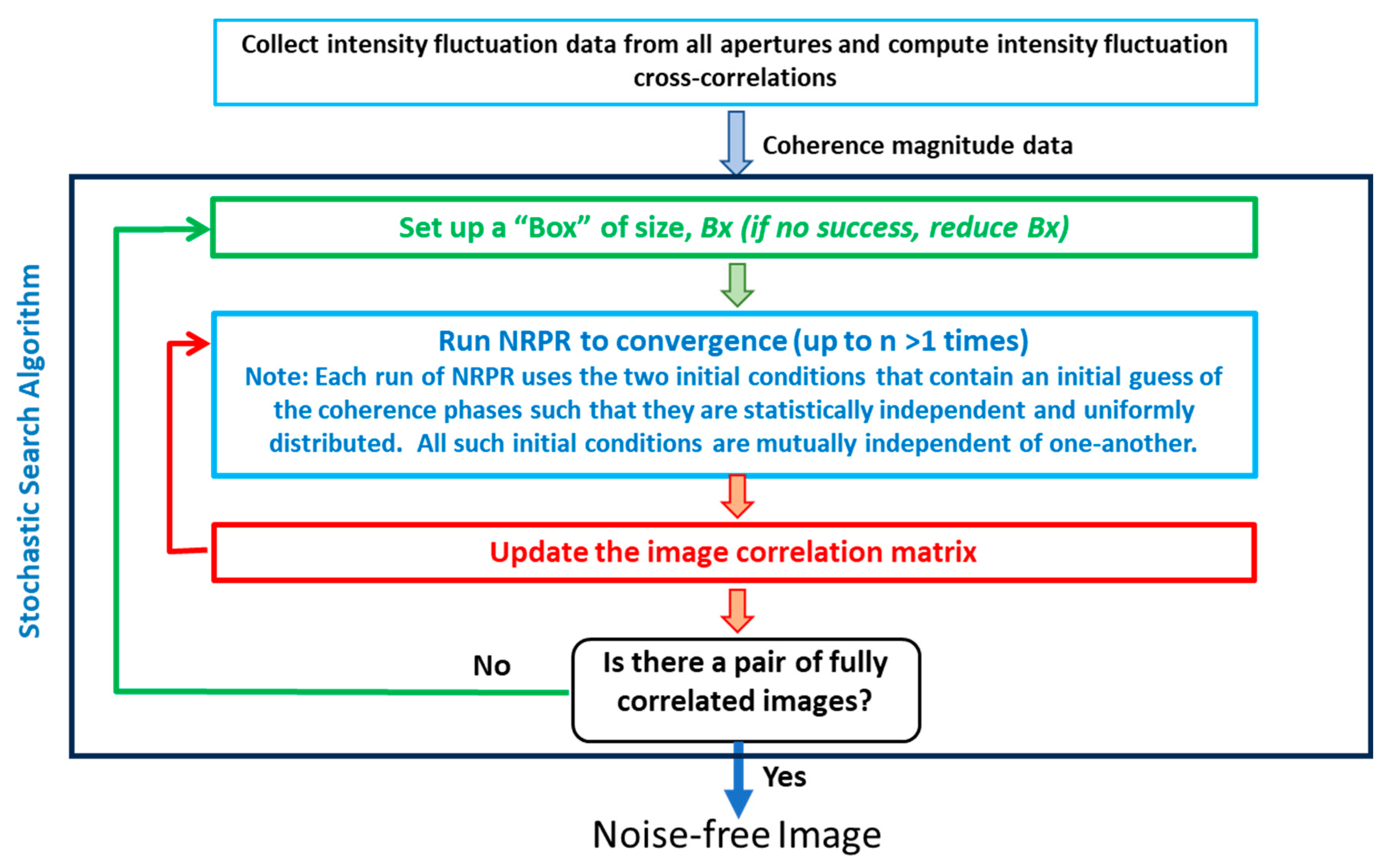
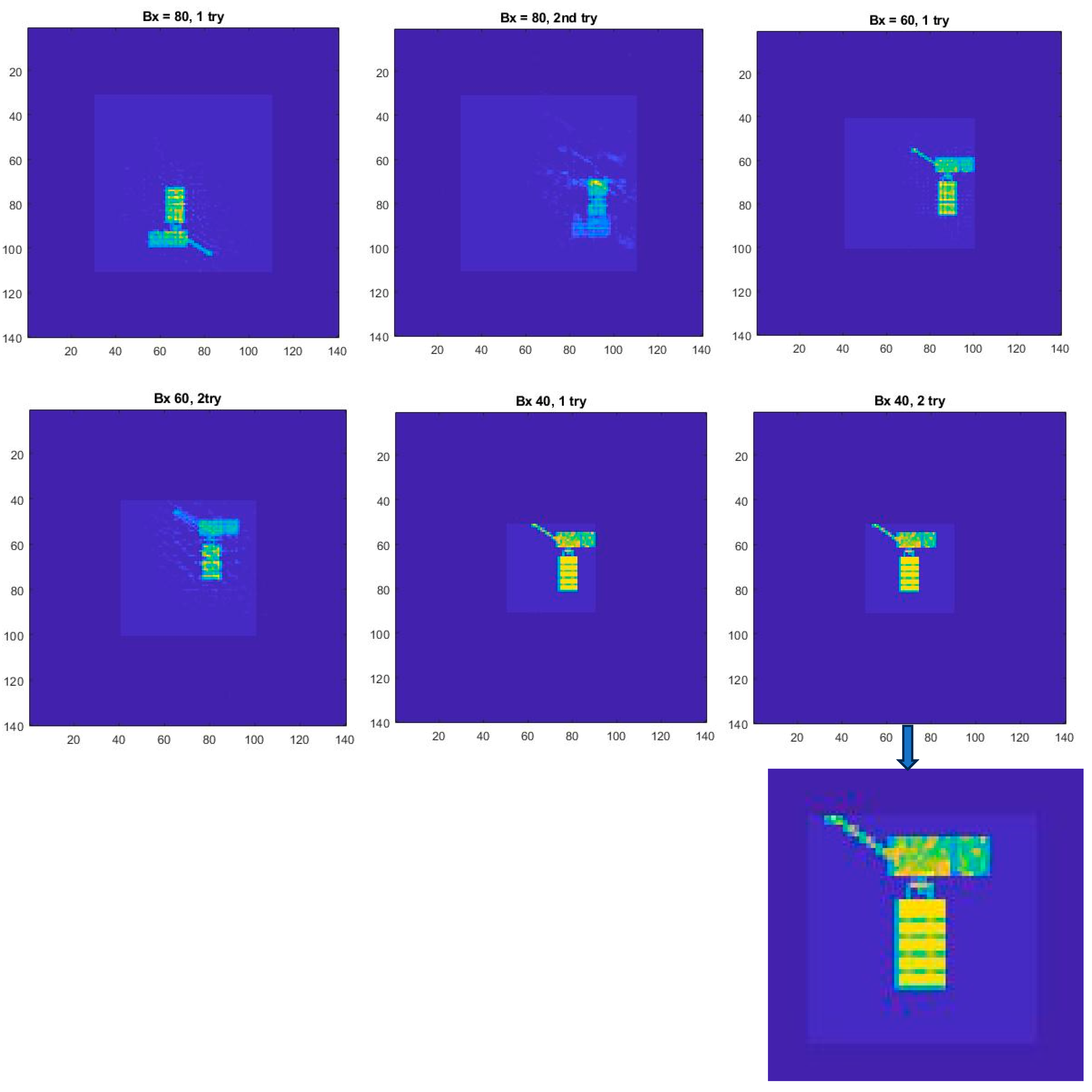
Given the nonnegative dynamic system, Section 5 merges the dynamic system within the stochastic search algorithm to gradually reduce the “box” sizes. In this formulation, we consider the stochastic search algorithm employing random coherence phases within the two initial conditions rather than random pixel intensities. The embedded NRPR runs use statistically independent and uniformly distributed coherence phases spanning $\left[-\pi ,\pi \right)$. The search sets up a square “Bx” and runs NRPR $n>1$ times until there are two images that are fully correlated. In this case, the two outcomes are the noise-free image (baring 180 degrees of rotation or translations). If there are no such correlations within n computations, then the algorithm reduces the box size and tries again. Alternately, a quicker convergence is to start with a box size that is smaller than the illuminated object and then increase the box sizes until the noise-free image is found.

Having explained how integration times are enormously reduced via a nonnegative dynamic system, Section 6 discusses the advantages of the ICI algorithm over other imaging technologies. We start with large-amplitude interferometry systems. These systems are still useful but are extremely complex in comparison with ICI. New, large facilities face an enormous cost barrier in comparison with ICI observatories, which are composed of inexpensive flux collectors and rapid integration times. Next, we consider adaptive optics. Adaptive optics remove the wavefront distortions introduced by the Earth’s atmosphere by means of an optical component that is introduced in the light beam, and which can introduce a controllable counter wavefront distortion that both spatially and temporally follows that of the atmosphere. We cite the following quotation:

“The application of adaptive optics to astronomical telescopes therefore requires the development of expensive, complex opto-mechanical devices and their control systems.”

Why is adaptive optics nearly extinct? ICI flux collectors are insensitive to atmospheric turbulence. Moreover, the flux collectors are exceedingly inexpensive.

Finally, a review of the Stellar Intensity Interferometry (termed SII) community is more promising. The apertures transmit intensity fluctuations to a computational facility where each pair of signals is cross-correlated in accordance with the Brown–Twiss formulation. In any case, SII is a steppingstone toward the incorporation of the ICI–stochastic search algorithm. In particular, basic SII can reduce integration times by means of redundant baseline measurements and multispectral channels. Such is also the case for ICI with the stochastic search algorithm. Furthermore, baseline redundancy and multispectral channels are entirely consistent with nonnegative dynamic systems.

In Section 7, we address a practical application, namely a ground-based imaging observatory design for commercial geostationary satellite inspection, focusing on apparent magnitudes of 10 to 14. In the process, we will compare the performance of both SII and ICI, in which the integration times of SII are ${10}^{10}$-fold larger than ICI integration times that range from 6 s to a few hours. Nor is the ICI satellite observatory incapable of high-resolution imaging of celestial objects. For example, there are numerous galaxies whose brightness is better than apparent magnitude 14. Comparing the James Webb Space Telescope and the ICI satellite observatory, the angular resolution is significantly better, and the JWST cost is enormously greater. This confirms the validity of the low-cost, streamlined, nonnegative ICI dynamic system.

2. Description of the NRPR Algorithm

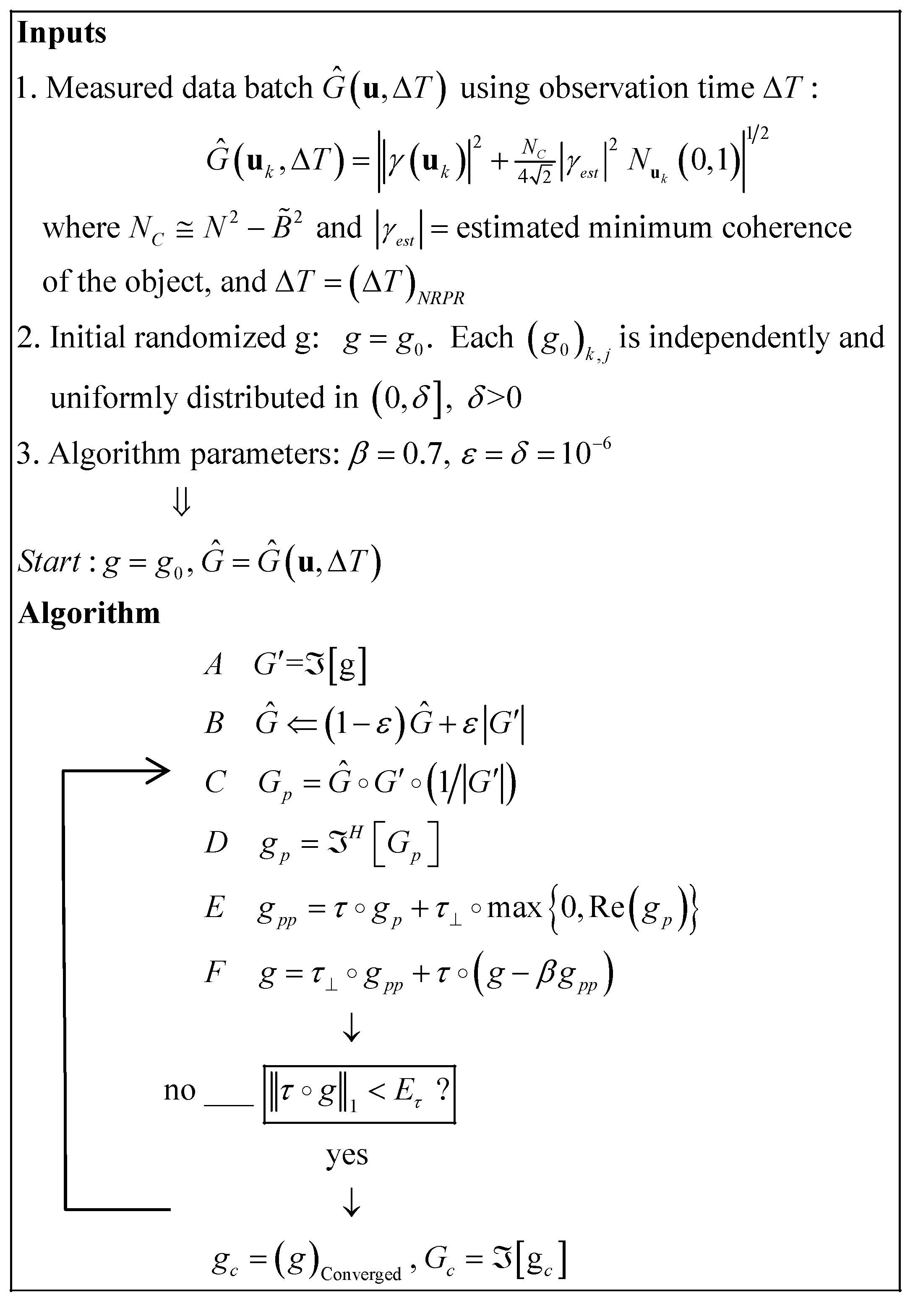
It is supposed that there is an array of flux-collecting apertures that are arranged so as to form a square, evenly spaced grid on the “u-v plane” (which, in interferometry, denotes the Fourier domain projected on the plane perpendicular to the target line of sight). The grid has a one-to-one correspondence to a matrix of $N\times N$ pixels forming the construction of an image of a luminous object amidst a black sky. The defining characteristics of the NRPR algorithm are as follows:

$$\begin{array}{l}g\in C^{N\times N}=\mathrm{Current} \mathrm{value} \mathrm{of} \mathrm{the} \mathrm{estimated} \mathrm{image} \left(\mathrm{pixellated}\right)\\ \overline{\mathrm{g}}\in R^{N\times N}=\mathrm{The} \mathrm{true} \mathrm{image}, \mathrm{without} \mathrm{noise}\\ \tau \in R^{N\times N}=\mathrm{Unity} \mathrm{for} \mathrm{pixels} \mathrm{constrained} \mathrm{to} \mathrm{have} \mathrm{zero} \mathrm{intensity}\\ \mathrm{and} \mathrm{zeros} \mathrm{for} \mathrm{pixels} \mathrm{that} \mathrm{are} \mathrm{unconstrained}\\ {\tau }_{\perp }\in R^{N\times N}={\mathrm{I}}_{N\times N}-\tau , \mathrm{the} \mathrm{opposite} \mathrm{of} \tau \\ \Im \left[\dots \right]=\mathrm{Two-dimensional} \mathrm{Fast} \mathrm{Fourier} \mathrm{Transform} \left(\mathrm{unitary}\right)\\ \overline{G}\in \Im \left[\overline{\mathrm{g}}\right]\in C^{N\times N}=\mathrm{The} \mathrm{measured} \mathrm{coherence} \mathrm{magnitudes} \mathrm{obtained}\\ \hspace{1em}\hspace{1em}\hspace{1em}\hspace{1em}\hspace{1em}\hspace{1em}\hspace{1em} \mathrm{by} \mathrm{cross-correlating} \mathrm{the} \mathrm{intensity} \mathrm{signals} \mathrm{from} \mathrm{all}\\ \hspace{1em}\hspace{1em}\hspace{1em}\hspace{1em}\hspace{1em}\hspace{1em}\hspace{1em} \mathrm{pairs} \mathrm{of} \mathrm{the} \mathrm{flux} \mathrm{collecting} \mathrm{apertures}\\ {\left(\Im \left[ \overline{\mathrm{g}}\right]\right)}_{kj}=\mathrm{FFT} \mathrm{in} \mathrm{the} \text{u-v} \mathrm{plane}, {\left(\Im \left[\overline{\mathrm{g}}\right]\right)}_{kj}={\left(\Im \left[\overline{\mathrm{g}}\right]\right)}_{kj}^{\ast }\\ \mathrm{Re}[\dots ]={\displaystyle \frac{1}{2}}\left([\dots ]+{[\dots ]}^{\ast }\right), \mathrm{the} \mathrm{real} \mathrm{valued} \mathrm{portion} \mathrm{of} [\dots ]\\ {\mathrm{Re}}_{+}[\dots ]=\max \left\{0,{\displaystyle \frac{1}{2}}\left([\dots ]+{[\dots ]}^{\ast }\right)\right\}, \mathrm{the} \mathrm{real} \mathrm{positive} \mathrm{of} [\dots ]\\ \left(A\right)\circ \left(B\right)= \mathrm{Hadamard} \mathrm{product} \mathrm{of} A \mathrm{and} B\end{array}$$

(2)

The matrix $\tau$ defines the set of constraints. ${\tau }_{kj}=1$ declares the pixels $\left(k,j\right)$ to be constrained to be zero, whereas ${\tau }_{kj}=0$ if $g_{k j}$ is unconstrained. The matrix ${\left({\tau }_{\perp }\right)}_{kj}$ is the opposite, with unity for unconstrained pixels and zero for constrained pixels. The region wherein ${\tau }_{kj}=1$ we have termed “the background”, and the remaining region “the foreground”. In this scenario, the initial inputs and the subsequent algorithm are defined as in Figure 1.

Figure 1 shows the various steps of the NRPR algorithm. There are several initial specifications. The first is the measured coherence magnitude, $\widehat{G}\left(u_k,\Delta T\right)={\left|{\left|\gamma \left(u_k\right)\right|}^2+\frac{N_C}{4\sqrt{2}}{\left|{\gamma }_{est}\right|}^2{N}_{u_k}\left(0,1\right)\right|}^{1/2}$, which obeys a positivity constraint. This is composed of the noise-free normalized coherence magnitude, $\left|\gamma \left(u_k\right)\right|$, where $u_k$ is the relative position vector of a pair of the flux-collecting apertures, $N_{u_k}\left(0,1\right)$ is a complex-valued Gaussian noise of zero mean and unit variance, and $N_C$ is the number of constrained pixels, i.e., $N_C={\displaystyle \sum _{k=1}^N{\displaystyle \sum _{j=1}^N{\tau }_{kj}}}\cong N^2$, as prescribed in the Introduction. In addition, the integration time, $\Delta T$, used for the NRPR integration time, is also related to Equation (1) and the appearance of the partial coherence effect. This will be considered in due course in a later Section. The formulation of this noise model was accomplished in [1], resulting in an asymptotic expression for the precision estimate of the necessary integration time. The third initial specification is $g=g_0$, where $g_0$ is independently and uniformly distributed in $\left(0,\delta \right]$, and $\delta$ is real and positive. It is these random specifications of the initial values of the pixel intensities that we wish to supplant with a dynamic system having additional simplifications. In passing, the closing of the image computation is measured in one norm of the magnitude of the pixel intensity. The image precision is measured by $E_{\tau }\le {10}^{-3}$.

It must be emphasized that only a single data batch of measured coherence magnitude measurements will be used in the process by which the zero-noise image is determined. Thus, the adaptive algorithms described here do not increase the necessary integration time. However, the adaptive algorithms require repeated NRPR computations, and each such repetition uses a new seed for the randomized initial guess for the image.

The various steps A to F of the algorithm are discussed in References [1,2,3]. We must note, however, that the parameter $\epsilon$ must equal ${10}^{-6}$ in order for step B to converge. Secondly, the parameter $\delta$ must also equal ${10}^{-6}$ in order to make step D converge. Now, there are two pathways to converge. There is the path depicted in Figure 1, in which $g_0$ is independently and uniformly distributed in $\left(0,\delta \right],\hspace{0.33em}\delta >0$. But there is a second path where the argument of the Fourier transform in Step A is independently and uniformly distributed. These two paths can be denoted as follows:

$$\delta \triangleq rand\left(N,N\right),\hspace{1em}\arg \left(G^{\prime }\right)\triangleq i\pi \left[2 rand(N,N)-1\right]$$

(3)

where $rand\left(N,N\right)$ is a set of independent and uniformly random variables in $\left(0,1\right]$. In order to create a nonnegative dynamic system, $\delta$ must equal $\epsilon$; they must both equal to ${10}^{-6}$. In the next Section, we must transform $\delta$ into the $\arg \left(G^{\prime }\right)$ path. Clearly, the phase factor, $e^{i\pi \left[2rand\left(N,N\right)-1\right]}$, in $\tau \circ g\left(0\right) \mathrm{and} {\tau }_{\perp }\circ g\left(0\right)$ is a statistical ensemble that encompasses all possible coherence phases. Thus, there is a very significant non-zero probability that in any one trial, NRPR converges to the correct coherence phase and magnitude, and therefore to the noise-free image.

Having obtained this transformation, the basic computations of NRPR are directed to the hypothesis that a square “box” of size $B_x$, and positioned in the center of the field of view, contains the noise-free image. Then, NRPR is embedded within the stochastic search wherein the hypothesis is tested, and the noise-free image is discovered.

3. The NRPR Algorithm as a Discrete-Time Dynamic System

As the next step in our analysis, we recast the equations of Figure 1 into a discrete-time dynamic system so that all the principal quantities are indicated by the sequence of integers $k=0,1,\dots \infty$. We start with the initial conditions and the first iteration, and recite the sequence of further iterations, keeping the algorithm in its proper order, as follows:

$$\begin{array}{c}\mathrm{g}\left(0\right)=\delta rand\left(N,N\right),\hspace{0.33em}\hspace{0.33em}\delta =\epsilon ={10}^{-6}\\ \widehat{G}(1)=\left(1-\epsilon \right)\widehat{G}\left(0\right)+\epsilon \left|\Im \left[\mathrm{g}\left(0\right)\right]\right|\\ k=0,1,2,\dots \infty \\ \Downarrow \\ G\left(k+1\right)=\Im \left[\mathrm{g}\left(k\right)\right]\\ \widehat{G}\left(k+1\right)=\left(1-\epsilon \right)\widehat{G}\left(k\right)+\epsilon \left|G\left(k+1\right)\right|\\ \tau \circ g\left(k+1\right)=\tau \circ \left\{g\left(k\right)-\beta \mathrm{Re}\left[{\Im }^H\left(\widehat{G}\left(k+1\right)\circ e^{i\arg \left(G\left(k+1\right)\right)}\right)\right]\right\}\\ {\tau }_{\perp }\circ g\left(k+1\right)={\tau }_{\perp }\circ {\mathrm{Re}}_{+}\left[{\Im }^H\left(\widehat{G}\left(k+1\right)\circ e^{i\arg \left(G\left(k+1\right)\right)}\right)\right]\end{array}$$

(4)

Now consider the equations pertaining to $k=0$ and $1$ and we note that the following equations are distinct from (4):

$$\begin{array}{c}G\left(1\right)=\Im \left[\delta rand\left(N,N\right)\right]=\delta e^{i\pi \left(2rand\left(N,N\right)-1\right)}\\ \widehat{G}\left(1\right)=\left(1-\epsilon \right)\widehat{G}\left(0\right)+\epsilon \delta \left|e^{i\arg \left(G(1)\right)}\right|\\ \tau \circ g\left(1\right)=\tau \circ \left\{\delta rand\left(N,N\right)-\beta \mathrm{Re}\left[{\Im }^H\left\{\left(1-\epsilon \right)\widehat{G}\left(0\right)\circ \left|e^{i\arg \left(G(1)\right)}\right|+\epsilon \delta \circ e^{i\arg \left(G(1)\right)}\right\}\right]\right\}\\ {\tau }_{\perp }\circ g\left(1\right)={\tau }_{\perp }\circ {\mathrm{Re}}_{+}\left[{\Im }^H\left\{\left(1-\epsilon \right)\widehat{G}\left(0\right)\circ \left|e^{i\arg \left(G(1)\right)}\right|+\epsilon \delta \circ e^{i\arg \left(G(1)\right)}\right\}\right]\end{array}$$

(5)

Notice that in (5), the quantities $e^{i\arg \left(G(1)\right)}$ are actually the factor $e^{i\pi \left(2 rand(N,N)-1\right)}$ in $G\left(1\right)$. We can replace $G\left(1\right)$ with $G\left(1\right)/\delta =\exp \left(i\pi \left(2 rand\left(N,N\right)-1\right)\right)$. Next, at the outset of the small $k$ integers, the second term in ${\widehat{G}}_{kj}(0)\triangleq {\left|{\left|{\gamma }_{kj}\right|}^2+\frac{N_C}{4\sqrt{2}}{\left|{\gamma }_{est}\right|}^2{N}_{kj}\left(0,1\right)\right|}^{1/2}$ dominates the expression with a huge contribution from $N_C$, regardless of the factor ${\left|{\gamma }_{est}\right|}^2$. Within the Fourier transform in (5), the term $\left(1-\epsilon \right)\widehat{G}\left(0\right)$ is of the order of at least hundreds, while the factor $\epsilon \delta \circ e^{i\arg \left(G(1)\right)}$ is of the order of ${10}^{-12}$.

Next, in the asymptotic analysis of Reference [3], the magnitude of $\tau \circ g\left(k\right)$ drops precipitately by an order of magnitude within $k\cong 25\triangleq k_T$. Pursuing the analysis in Reference [3] further, we focus on the average magnitude of the image intensity of the background, namely $〈g_b\left(k\right)〉\triangleq \frac{1}{N^2-B_x^2}{\displaystyle \sum _{m=1}^{N^2-B_x^2}{\left|g_b\left(k\right)\right|}_m}$. The Kronecker algebra in Reference [3] results in the following outcomes: (1) at $k\cong 25\triangleq k_T$, the magnitude of the average of $\left|\tau \circ \left\{\delta rand\left(N,N\right)\right\}\right|$ is zero; (2) for $k_T,\dots ,\infty$ the magnitude of the average of $\mathsf{\Theta }\triangleq \beta \left|\tau \circ {\Im }^H\left\{\left(1-\epsilon \right)\widehat{G}\left(k_T,\dots ,\infty \right)\circ \left|e^{i\arg \left(G(k_T+1,\dots ,\infty )\right)}\right|\right\}\right|$ is completely controlled by $\epsilon$. The combination of (1) and (2) implies that (2) cannot contain $\delta$, meaning that there are no high-order terms in $\mathsf{\Theta }$. However, the average of $\left|\tau \circ \left\{\delta rand\left(N,N\right)\right\}\right|$ from $k=0 \mathrm{to} k_T$ must contain $\epsilon \delta$, since the average of $\left|\tau \circ \left\{\delta rand\left(N,N\right)\right\}\right|$ varies smoothly from its initial condition to zero (see Figure 2 and Figure 3). Therefore, it follows that the only increment to the magnitudes of the terms $\left|\epsilon \delta \circ e^{i\arg \left(G(k_T)\right)}\right|$ must approximately accumulate to $\frac{1}{2}{k}_T\left|\epsilon \delta \circ e^{i\arg \left(G(k_T)\right)}\right|\cong 12\times {10}^{-12}$. As the image precision is ${10}^{-3}$, it is thus clear that this accumulation is extremely negligible and that all the terms $\left|\epsilon \delta \circ e^{i\arg \left(G(1)\right)}\right|$ can be discarded at the outset to produce Equation (6); moreover, the deletion of $\epsilon \delta$ is well-founded. Again, Equation (6) are transformations of (5).

$$\begin{array}{c}\arg \left(G\left(1\right)\right)=\pi \left(2 rand\left(N,N\right)-1\right)\\ \widehat{G}\left(1\right)=\left(1-\epsilon \right)\widehat{G}\left(0\right)\\ \tau \circ g\left(1\right)=\tau \circ \left\{\delta rand\left(N,N\right)-\beta \mathrm{Re}\left[{\Im }^H\left\{\left(1-\epsilon \right)\widehat{G}\left(0\right)\circ \left|e^{i\arg \left(G(1)\right)}\right|\right\}\right]\right\}\\ {\tau }_{\perp }\circ g\left(1\right)={\tau }_{\perp }\circ {\mathrm{Re}}_{+}\left[{\Im }^H\left\{\left(1-\epsilon \right)\widehat{G}\left(0\right)\circ \left|e^{i\arg \left(G(1)\right)}\right|\right\}\right]\end{array}$$

(6)

We can see that there is a bifurcation into two dynamic systems: one involving $\delta$, and the rest consisting of $\epsilon$. Now, let us examine k = 1 formulated as the initial conditions. First, we may eliminate $\epsilon$ in $\widehat{G}\left(1\right)=\left(1-\epsilon \right)\widehat{G}\left(0\right)$, because $\epsilon$ is a very small shift and $\widehat{G}\left(0\right)$ can be easily adjusted by a slight change in $N_C$. Thus, we can formulate the initial conditions for k = 2, as follows:

$$\begin{array}{c}{\widehat{G}}_{kj}(1)={\widehat{G}}_{kj}(0)\\ \tau \circ g\left(1\right)=\tau \circ \left\{\delta rand\left(N,N\right)-\beta \mathrm{Re}\left[{\Im }^H\left\{\widehat{G}\left(1\right)\circ \left|e^{i\pi \left[2 rand\left(N,N\right)-1\right]}\right|\right\}\right]\right\}\\ {\tau }_{\perp }\circ g\left(1\right)={\tau }_{\perp }\circ {\mathrm{Re}}_{+}\left[{\Im }^H\left\{\widehat{G}\left(1\right)\circ \left|e^{i\pi \left[2 rand\left(N,N\right)-1\right]}\right|\right\}\right]\end{array}$$

(7)

However, turning back to (4), we can complete the entire sequence starting from k = 1:

$$\begin{array}{c}{\widehat{G}}_{kj}\left(1\right)={\widehat{G}}_{kj}\left(0\right)\\ \tau \circ g\left(1\right)=\tau \circ \mathrm{Re}\left[\delta rand\left(N,N\right)-\beta {\Im }^H\left\{ \widehat{G}\left(0\right)\circ e^{i\pi \left[2rand\left(N,N\right)-1\right]}\right\}\right]\\ {\tau }_{\perp }\circ g\left(1\right)={\tau }_{\perp }\circ {\mathrm{Re}}_{+}\left[{\Im }^H\left(\widehat{G}\left(0\right)\circ e^{i\pi \left[2rand\left(N,N\right)-1\right]}\right)\right]\\ \Downarrow \mathrm{k}=1,2,\dots ,\infty \\ \widehat{G}\left(k+1\right)=\left(1-\epsilon \right)\widehat{G}\left(k\right)+\epsilon \left|\Im \left[\mathrm{g}\left(k\right)\right]\right|\\ \tau \circ g\left(k+1\right)=\tau \circ \left\{g\left(k\right)-\beta \mathrm{Re}\left[{\Im }^H\left(\widehat{G}\left(k+1\right)\circ e^{i\arg \left(\Im \left[\mathrm{g}\left(k\right)\right]\right)}\right)\right]\right\}\\ {\tau }_{\perp }\circ g\left(k+1\right)={\tau }_{\perp }\circ {\mathrm{Re}}_{+}\left[{\Im }^H\left(\widehat{G}\left(k+1\right)\circ e^{i\arg \left(\Im \left[\mathrm{g}\left(k\right)\right]\right)}\right)\right]\end{array}$$

(8)

These equations are transformations of (4)–(7). This dynamic system replaces six steps per iteration with three steps. Note that the quantity $e^{i\pi \left[2rand\left(N,N\right)-1\right]}$ is the phase factor of the Fourier transform of the random initial pixel intensities. The new initial conditions in Equation (8) are correct within $k_T\epsilon \delta$ (${10}^{-12}$). In particular, one must note that (8) also leads to the convergence of $\tau \circ g\left(k\right)$ to zero, as demonstrated in Reference [3]. Therefore, in the limit, ${\tau }_{\perp }\circ g\left(k\right)$ is the ultimate nonnegative dynamic system, which is discussed in the next section.

4. Two Dynamics: The Reduction of $\mathit{\tau }$ and the Affirmation of ${\mathit{\tau }}_{\mathbf{\perp }}$

The first step in setting up the stochastic search algorithm is to hypothesize a square perimeter with size $B_x$. The exterior of the box is where we find the constrained pixels, called the “background”, whereas the interior of the box is the “foreground”, wherein all pixels are determined to have ${\tau }_{\perp }=1$. Starting from the initial conditions in (8), the dynamic system must be able to converge to zero background pixels. Once that is completed, the dynamic system can converge to strict nonnegative-intensity pixels. Each run of NRPR can produce similar results using the same initial conditions, until a pair of images are found that are completely correlated, indicating the true, noise-free image.

To determine the convergence of the background pixels, we use the Kronecker vector notation on (8). $g\left(k\right)$ is represented by the following column vector:

$$g\left(k\right)=\left(\begin{array}{c}{g}_b\left(k\right)\\ g_f\left(k\right)\end{array}\right),\hspace{1em}{g}_b\left(k\right)\in {ℝ}^{N^2- B_x^2},\hspace{1em}{g}_b\left(k\right)\in {ℝ}^{B_x^2}$$

(9)

In other words, $g_b\left(k\right)$ is a vector composed of the matrix elements of the background pixels, and $g_f\left(k\right)$ is the vector composed of the matrix elements of the foreground pixels. Corresponding to this, we have the following:

$$G\left(k\right)\triangleq \Im \left[\mathrm{g}\left(k\right)\right]=\left[\begin{array}{cc}{F}_b& F_{bf}\\ F_{bf}^H& F_f\end{array}\right]\left(\begin{array}{c}{g}_b\left(k\right)\\ g_f\left(k\right)\end{array}\right),\hspace{1em}\widehat{G}\left(k\right)=\left(\begin{array}{c}{\widehat{G}}_b\left(k\right)\\ {\widehat{G}}_f\left(k\right)\end{array}\right)$$

(10)

$\left[\begin{array}{cc}{F}_b& F_{bf}\\ F_{bf}^H& F_f\end{array}\right]$ is the unitary matrix corresponding to the Fourier transform operator in the Kronecker notation. Finally, $\tau$ is represented by the following:

$$\tau =\left[\begin{array}{cc}{I}_{N^2-B_x^2}& 0\\ 0& 0\end{array}\right]$$

(11)

In Reference [3], an asymptotic approximation of the background was computed, introducing the averages of $g_b\left(k\right)\in {ℝ}^{N^2-B_x^2},\hspace{1em}{g}_b\left(k\right)\in {ℝ}^{B_x^2}$ as defined below:

$$〈g_b\left(k\right)〉\triangleq \frac{1}{N^2-B_x^2}{\displaystyle \sum _{m=1}^{N^2-B_x^2}{\left|g_b\left(k\right)\right|}_m}\hspace{0.33em}\hspace{0.33em}〈g_f\left(k\right)〉\triangleq \frac{1}{B_x^2}{\displaystyle \sum _{m=1}^{B_x^2}{\left|g_f\left(k\right)\right|}_m}$$

(12)

For the first order, the maximum estimate for the limit on $〈g_b\left(k\right)〉$ can be found as follows:

$$G_f\left(k\right)\cong \left(1+\alpha \epsilon k\right)\left|{\widehat{G}}_f\left(k\right)\right|,\hspace{1em}\alpha \cong 10$$

(13)

The resulting asymptotic approximation is as follows:

$$\begin{array}{c}〈g_b\left(k+1\right)〉=\left(1-\frac{1}{4}\beta \right)〈g_b\left(k\right)〉+\frac{1}{2}\beta \frac{A}{N^2\left(1+\alpha \epsilon k\right)}〈g_b\left(0\right)〉\\ 〈g_b\left(k=0\right)〉\cong 0.05,\hspace{0.33em}A={\left(30\right)}^2,\hspace{0.33em}N=140,\hspace{0.33em}\alpha =10\end{array}$$

(14)

The computations for the first 40 iterations are shown in Figure 2 and Figure 3 gives the complete 7000 iterations.

A comparison of the predicted and computed results in Figure 2 and Figure 3 establishes that the averaged background intensity is reduced by one order of magnitude at the outset, and then levels off beyond iterate $k=k_T\cong 25$ to form a floor that does not vary appreciably beyond $k=k_T$. However, Figure 3 shows that after $k=k_T\cong 25$, the reduction in $〈g_b\left(k\right)〉$ is completely driven by $\epsilon$. These features match the computed results rather well, especially for the immediate drop-off for $k<k_T$, where it is established that $〈g_b\left(k\right)〉$ is very weakly dependent on $B_x$. Figure 3 shows the complete averaged background from k = 1 to k = 7000.

The conclusion of this derivation is that after $k=k_T$, $g_b\left(k\right)$ is so suppressed relative to $g_f\left(k\right)$, its influence on the foreground may be neglected. Thus, we set $g_b\left(k\right)\cong 0, \mathrm{and} \left[\begin{array}{l}{G}_b\left(k\right)\\ G_f\left(k\right)\end{array}\right]\cong \left[\begin{array}{cc}0& 0\\ 0& F_f\end{array}\right]\left(\begin{array}{c}{g}_b\left(k\right)\\ g_f\left(k\right)\end{array}\right)$, so that in Kronecker notation, (8) becomes the following:

$$\begin{array}{c}\arg \left(F_f{g}_f\left(k_0\right)\right)\cong \pi \left[2rand\left(B_x,B_x\right)-1\right]\\ k=k_0,\hspace{0.33em}{k}_0+1,\hspace{0.33em}{k}_0+1,\dots ,\infty \\ \downarrow \\ {\widehat{G}}_f\left(k+1\right)={\widehat{G}}_f\left(k\right)+\epsilon \left(\left|F_f{g}_f\left(k\right)\right|-{\widehat{G}}_f\left(k\right)\right)\\ g_f\left(k+1\right)={\mathrm{Re}}_{+}\left\{F_f^H\left[{\widehat{G}}_f\left(k+1\right)\circ e^{i\arg \left(F_f{g}_f\left(k\right)\right)}\right]\right\}\\ \end{array}$$

(15)

Thus, as $k\to \infty$, $g_b\left(k\right)\to 0$ and both $g_f\left(k\right)$ and ${\widehat{G}}_f\left(k\right)$ constitute a nonnegative dynamic system.

5. The Stochastic Search Algorithm for Sequential Box Sizes

In this Section, we consider the stochastic search algorithm employing random coherence phases within the two initial conditions rather than random pixel intensities. Figure 4 shows that the embedded NRPR runs (in blue) use statistically independent and uniformly distributed coherence phases spanning $\left[-\pi ,\pi \right)$. The search sets up a square “Bx” and runs NRR $n>1$ times until there are two images that are fully correlated. In this case, the two outcomes are the noise-free image (baring 180 degrees of rotation or translations). If there are no such correlations within n computations, then the algorithm reduces the box size and tries again. If, by chance, a converged image has pixel intensities that reside outside of the box, this indicates that the box is too small to contain the illuminated object, and the box size must be enlarged. Overall, this is the process by which the stochastic search validates the hypotheses of the box size.

In Figure 5, we demonstrate that the dynamic system (15) behaves essentially the same as in References [1,2,3], when the smallest box size fully contains the illuminated object. Alternately, one can start with a box size that is smaller than the illuminated object and then increase the box sizes until the noise-free image is found. With this strategy, the number of NRPR computations is distinctly reduced. In fact, if the number of runs is large for the decreasing box size, then for the same image, the number of runs for the increasing box sizes is halved. The latter strategy, as mentioned in Reference [3], is clearly superior. Figure 6 illustrates the superior path.

6. Advantages over Other Two-Dimensional Imaging Methods

Now that integration times are enormously reduced, we can appreciate the benefits of ICI over previous imaging technologies. We may start with optical interferometer telescopes and refer the reader to the technical background in Reference [4]. ICI does not require the propagation of collected light beams to combiner units as in existing amplitude interferometers. The ICI hardware consists of simple, self-contained flux collectors that are immune to seeing conditions and need not collect phase information. Thus, routing optics and beam combiners are eliminated, thereby saving a great deal of expense. ICI does not require nanometer-level control of nor nanometer knowledge of the relative positions of the optical components. While margins for optical components in amplitude interferometry are a small fraction of a wavelength, ICI margins are in the centimeter range. Finally, the signal-to-noise ratio (SNR) does not suffer from beam splitting and the throughput losses that plague amplitude interferometry. These remarks indicate a great deal of performance advantages with a corresponding reduction in expense.

Next, we consider adaptive optics. Reference [5] provides an excellent overview. Adaptive optics remove the wavefront distortions introduced by the Earth’s atmosphere by means of an optical component which is introduced in the light beam, and which can introduce a controllable counter wavefront distortion which both spatially and temporally follows that of the atmosphere. This optical component is generally a mirror whose surface can be distorted. To control the mirror, the wavefront distortions have to be known. These are measured by means of a wavefront sensor using either the object under study or a laser-generated object. In the case where the wavefront is measured with the required accuracy and spatial and temporal resolution, and in which the adaptive mirror control is perfect, the atmospheric effects are removed, and the telescope will give a diffraction-limited image. Reference [5] states that “The application of adaptive optics to astronomical telescopes therefore requires the development of expensive, complex opto-mechanical devices and their control systems.” Why is adaptive optics nearly extinct? We answer that ICI flux collectors are insensitive to atmospheric turbulence. Moreover, the flux collectors are exceedingly inexpensive.

Finally, a review of Stellar Intensity Interferometry (termed SII) [6] extolls the virtues of the basic Brown–Twiss technology. The apertures transmit intensity fluctuations to a computational facility where each pair of signals is cross-correlated in accordance with the Brown–Twiss formulation. It is acknowledged that the weak signals must be boosted via an array of large apertures (i.e., the VERITAS array), but it is not certain that the partial coherence factor has been included. In any case, SII is a steppingstone toward the incorporation of the ICI–Stochastic Search algorithm. The SII community has made significant progress over the last few decades. In particular, the basic SII can reduce integration times by means of redundant baseline measurements [7,8]. These measurements are composed of radial baselines appropriate to stellar diameter computations, but it is easy to adopt the two-dimensional, baseline redundancy featured in Section 7. Also, of course, multiple spectral channels are introduced in Reference [9]. Such is also the case for ICI with the stochastic search algorithm. Progress has also been made in the area of photonic integrated circuits that have been adapted to visible light, [10,11,12] and fitted with Avalanche Photodiodes [13] to produce enormous bandwidths [14]. In view of this progress, it makes good sense to couple the SII community with the ICI–stochastic search algorithm. Furthermore, baseline redundancy and multispectral channels are entirely consistent with nonnegative dynamic systems. In the following Section, we address a practical application, namely an imaging observatory design for commercial geostationary satellite inspection. In the process, we will compare the performance of both SII and IC and their combination.

7. Observatory Design for Commercial Geostationary Satellite Inspection

This section addresses the characteristics of a ground-based observatory suited to the high-resolution imaging of commercial geostationary satellites, as treated in [10]. The first consideration is the range of apparent magnitudes. Many of the smaller scale satellites range in magnitude from 10 to 14. These are also typical of GOES 16-sized bodies. Therefore, we select a satellite that is 6 by 6 m, exhibiting the apparent magnitudes, $m_{sat}$, in the range of 10 to 14. We wish to achieve a fairly challenging degree of image resolution. Accordingly, we choose a resolution, $\Delta x$, of 10 cm in size. This is an angular resolution of 2.8 $\mu rad$.

For simplicity, it is assumed that the tilt of the u-v plane from zenith is modest, so that the positioning of the observatory apertures is approximately on the horizontal ground plane. The geometry of the observatory is defined by the location vectors, termed here as the baseline vectors, linking all the pairs of aperture locations in the horizontal plane. Each baseline vector is associated with the time averaged, intensity fluctuation cross-correlation (i.e., the coherence magnitude data) collected by the aperture pairs.

In the SII community, the integration time reduction due to baseline redundancy has been well-treated within a one-dimensional setting [7,8]. In imaging, it is our task to extend the analysis to the much more complex u-v plane. The reward, however, is that the integration times are enormously reduced in the two-dimensional setting—both in the SII and the ICI settings.

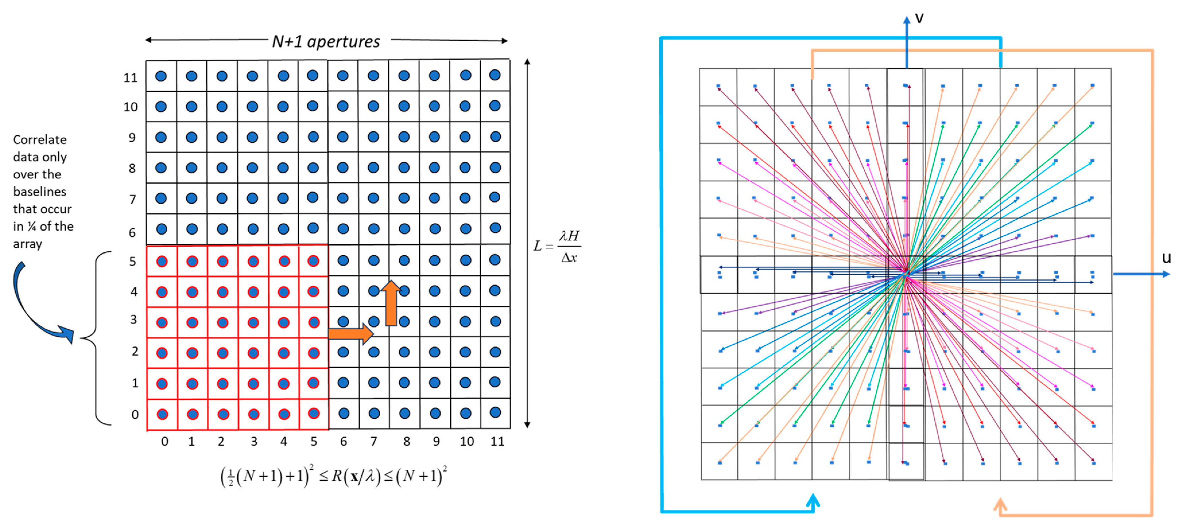
To estimate the further reduction in integration time, it is assumed that the aperture positions occupy a square grid. If there were no baseline redundances, the image plane and the u-v plane would be one-fourth the size of the aperture grid. However, we can make the aperture grid four times larger than the u-v plane. This implies a square grid for both the aperture grid and the u-v plane, as well as the desired image field of view. In the latter case, the size of the image is denoted by $N$ pixels on the side, where $N$ is an odd integer. The following discussion demonstrates how a square grid of aperture positions that are $N+1$ on one side can produce a significant reduction in integration time by means of redundant baseline vectors.

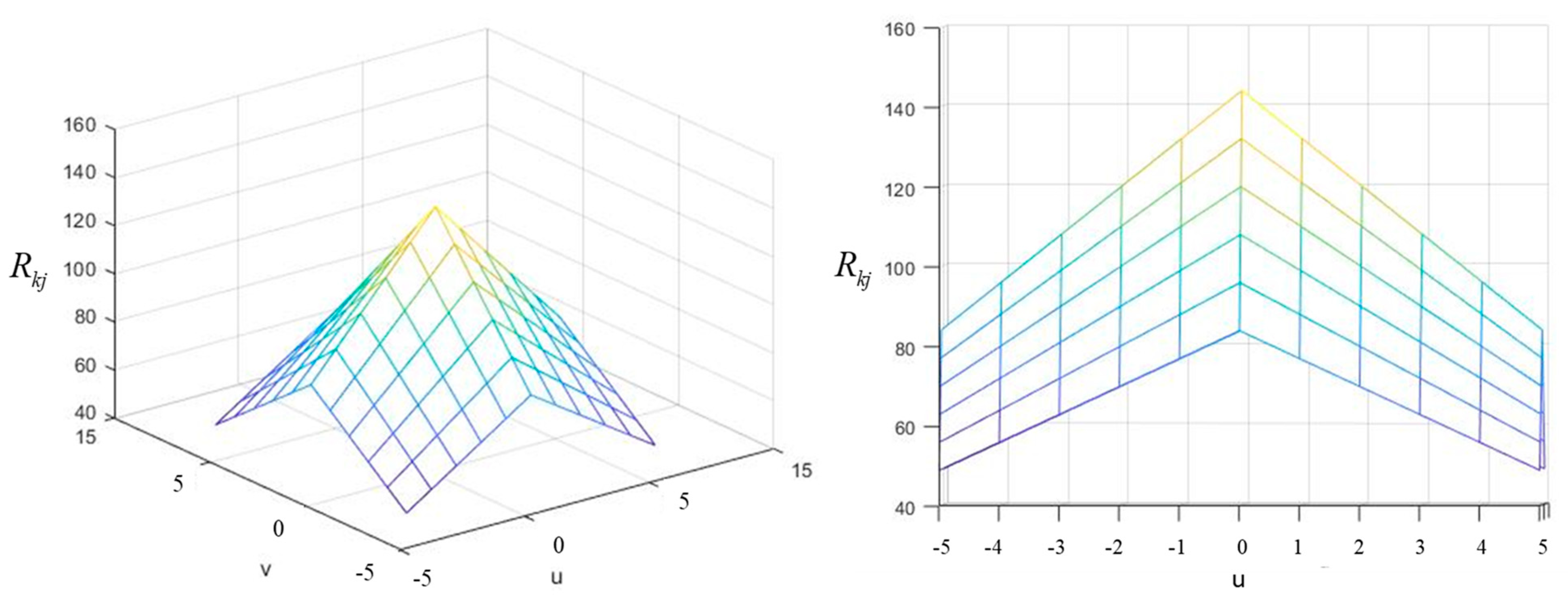
To begin, we use Figure 7 to explain the process, where $N=11$. The figure shows ${\left(N+1\right)}^2={12}^2$ apertures in a square array. We take one-fourth of this array, shown by the red outlines, and compute the intensity fluctuation cross-correlations for all the baseline vectors in the $\left(N+1\right)/2 \mathrm{by} \left(N+1\right)/2$ region. Then, we reposition this array within the $\left(N+1\right) \mathrm{by} \left(N+1\right)$ array without repeating any position and without repeating a cross-correlation for a 180-degree rotation of a baseline vector. As is described in Appendix A of [10], which explains the computational aspects of the design, all of these calculations are readily parallelizable, and therefore can be produced within the same integration time. Given these cross-correlation data, we can construct an $\left(N+1\right)/2 \mathrm{by} \left(N+1\right)/2$ array, where for each of the fundamental baselines the sample averages of the redundant coherence magnitude measurements are assigned.

The resulting redundancy matrix for our $N=11$ example is shown in Figure 8. In general, for each u-v vector, $u$, the redundancy, denoted by $R\left(u\right)$, is determined as follows:

$$U\in {ℝ}^{N+1}: \hspace{0.33em}U=\left[1,\dots ,1\right] M\triangleq \left[\begin{array}{ccc}0& 0& 0\\ 0& U^{T}U& 0\\ 0& 0& 0\end{array}\right]$$

(16)

$$R\left(u\right)={\left[\begin{array}{c}0\\ I_N\\ 0\end{array}\right]}^T\left\{M\circ \left\{F^H\left[{\left|F\left[M\right]\right|}^2\right]\right\}\right\}\left[\begin{array}{c}0\\ I_N\\ 0\end{array}\right]$$

(17)

We note the following:

$${\left(\frac{1}{2}\left(N+1\right)+1\right)}^2\le R\left(u\right)\le {\left(N+1\right)}^2$$

(18)

According to [10], the integration time is as follows:

$$\begin{array}{c}\Delta T\left(u\right)={\displaystyle \frac{1}{R\left(u\right)}}{\left[{\displaystyle \frac{4}{N_C{S}_0{\left|\gamma \left(u\right)\right|}^2}}\right]}^2={\left\{\Delta T\left(u\right)\right\}}_{NRPR}\\ S_0=\eta \overline{\beta }\sqrt{\Delta {\nu }_d}P\left(A\right)\end{array}$$

(19)

where

$$\begin{array}{l}\overline{\beta }=\mathrm{Number} \mathrm{density} \mathrm{per} \mathrm{mode}\hspace{0.33em}\cong AI{T}_c \\ A=\mathrm{Aperture} \mathrm{area}\\ I=\mathrm{Number} \mathrm{of} \mathrm{photon} \mathrm{arrivals}/s-m^2\\ T_c=\mathrm{Correlation} \mathrm{time} \mathrm{of} \mathrm{the} \mathrm{light}\\ \Delta {\nu }_d=\mathrm{Bandwidth} \mathrm{of} \mathrm{the} \mathrm{detector}\\ \eta =\mathrm{Photon} \mathrm{detection} \mathrm{efficiency}\\ P\left(A\right)=\mathrm{Partial} \mathrm{coherence} \mathrm{effect}\\ N_C=\mathrm{Number} \mathrm{of} \mathrm{constrained} \mathrm{pixels}\end{array}$$

(20)

An additional method that results in decreased integration time is to equipe each photodetector with multiple non-overlapping frequency channels (so that all channels are statistically independent), denoted here by $M_c$. One then averages the detector output channels. Workers in SII [9], have studied multispectral theory with good, albeit modest, results. For two-dimensional imaging with ICI, reference [10] introduces a multispectral approach pertaining to Geostationary Satellite Inspection. This adopts a more recent approach which exploits rapid advances in photonic integrated circuits (PIC). Programmable PICs have been adapted to visible light [11,12] and combined with Avalanche Photodiode (APD) electronics [13] to produce photodetectors with enormous bandwidths [14] (published June 2023). In consequence, for each photodetector, we adopt an APD with a PIC that separates broadband light into numerous (~1000 channels), non-overlapping and equal-bandwidth spectral channels. Since the Fock states of each channel commute, the channels are mutually statistically independent. The correlation data are then computed for each pair of apertures and for each corresponding spectral channel, and the results are averaged.

Reference [10] discusses the state of the art in multispectral detectors that admits reasonably priced and modest numbers of frequency channels. Within the present state of the art, if $\Delta {\nu }_d=1\hspace{0.33em}GHz$, one can sustain 600 channels. With future advances in PICs, we estimate that many more channels can be supplied, but this requires further development and price reduction. Therefore, we concentrate on the 600 channel devices.

Thus, Reference [10] gives us the following:

$$\begin{array}{c}\Delta T\left(u\right)\cong {\displaystyle \frac{1}{M_c}}{\left[{\displaystyle \frac{1}{\left[\frac{1}{2}\left(N+1\right)+1\right]}}{\displaystyle \frac{4}{S_0{\left|\gamma \left(u\right)\right|}_{\min }^2}}\right]}^2={\left\{\Delta T\left(u\right)\right\}}_{NRPR}\\ S_0=\eta \overline{\beta }\sqrt{\Delta {\nu }_d}P\left(A\right)\end{array}$$

(21)

Now we take account of the parameters needed for the integration time computations. First, ref. [10] stipulates that $N\cong \left(3/\Delta x\left(m\right)\right)\times 6 m\cong 2000$. This leads to the following:

$$\begin{array}{c}L\triangleq \mathrm{Length} \mathrm{of} \mathrm{the} \mathrm{side} \mathrm{of} \mathrm{the} \mathrm{aperture} \mathrm{grid}=179 m\\ d\triangleq \mathrm{Diameter} \mathrm{of} \mathrm{the} \mathrm{square} \mathrm{flux} \mathrm{collector}=L/\left(N+1\right)=9 cm\end{array}$$

(22)

The reason why the equation $S_0=\eta \overline{\beta }\sqrt{\Delta {\nu }_d}P\left(A\right)$ was placed near all the $\Delta T\left(u\right)$ expressions is that the partial coherence effect, $P\left(A\right)$, is precisely satisfied by $d=9 \mathrm{cm}$, thanks to the Brown–Twiss integration [15]. The flux collectors are the size of flashlights. Next, the additional parameters are as follows:

$$\begin{array}{c}H\triangleq \mathrm{Altitude}=35,786 km\\ \eta \triangleq \mathrm{Detector} \mathrm{efficiency}=0.5\\ \Delta {\nu }_d\triangleq \mathrm{Detector} \mathrm{bandwidth}=1 GHz\hspace{0.33em}\\ \hspace{0.33em}{\left|\gamma \right|}_{\min }\triangleq \mathrm{Minimum} \mathrm{normalized} \mathrm{coherence} \mathrm{magnitude}={10}^{-3}\\ N_C\triangleq \mathrm{Number} \mathrm{of} \mathrm{constrained} \mathrm{pixels}=\frac{8}{9}{N}^2\\ \overline{\beta }\triangleq \mathrm{number} \mathrm{density} \mathrm{per} \mathrm{mode}=\mathrm{A} \mathrm{function} \mathrm{of} m_{sat}\end{array}$$

(23)

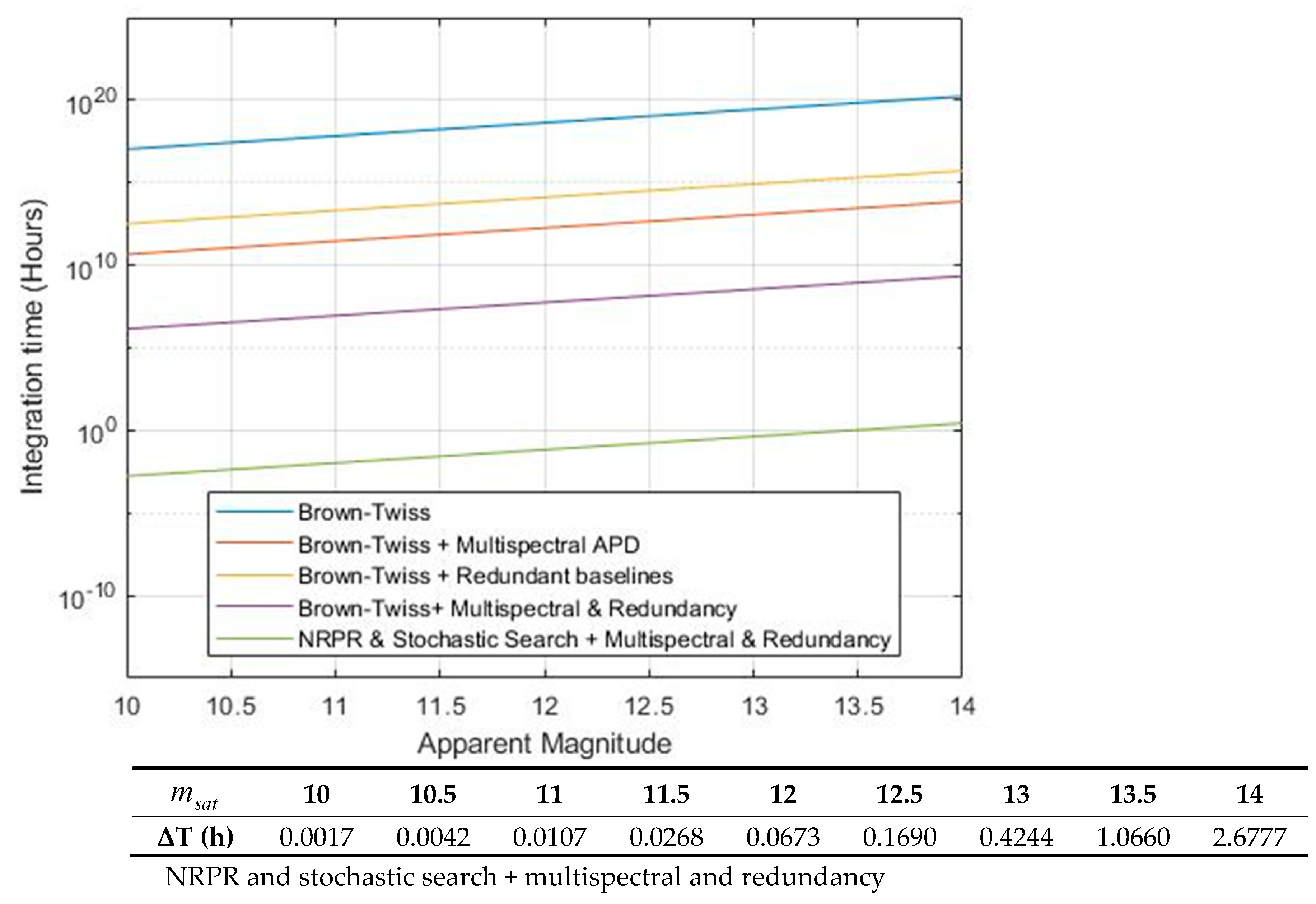
With these parameters, we can plot the integration times versus the apparent magnitudes for various combinations of Brown–Twiss integration times with redundant baselines, multispectral channels, and a combination of NRPR and stochastic search with multispectral and baseline redundancy.

The blue line in Figure 9 shows the conventional Brown–Twiss integration times. Then, the red and yellow lines are the conventual Brown–Twiss with separate multispectral APDs and redundant baselines. Each of these are more or less comparable. Then, the violet line features Brown–Twiss conventions with both multispectral and redundant baselines simultaneously. This represents the full-force SII integration times. Note that this line still does not, by any means, bring the integration times down to the level of an hourly integration time limit. On the contrary, the SII integration times are roughly ${10}^{10}$ times larger than the green line that represents the NRPR and stochastic search combined with the multispectral and redundant baselines. Thus, to achieve low integration times, the NRPR and Stochastic algorithm is absolutely necessary.

Furthermore, the ICI Satellite observatory can also outperform the James Webb Space Telescope (JWST) in imaging galaxies that are brighter than the apparent magnitude 14, as shown in the following

Table 1. The number of galaxies that are brighter than apparent magnitude 14: $\sim 2\times {10}^6$.

Performance Parameter	JWST	ICI Satellite Observatory
OTE diameter (meters)	6.1 by 6.6	179 by 179
Unobscured aperture (SQ meters)	25	32,041
Telescope field of view (arc min)	18 by 9	18/3600 km
Wavelength of diffraction limited performance	2	0.5
Resolution	0.315	0.008
Cost (USD)	~10,000 million	~16 million

. The observatory is enormously larger than JWST, and due to its size and its wavelengths in the visible spectrum, the image resolution is 0.025 that of the space telescope. Then, there is the relative cost between USD 10 billion and USD 16 million. JWST is extremely complex, while the ICI ground-based observatory has the same immunity to atmospheric seeing conditions and is composed of an array of self-contained flux collectors (the size of which is that of a small flashlight), each of which is equipped with inexpensive multispectral channels. The flux collectors transmit intensity fluctuations to an onsite, highly parallelized computational facility where all the pairs of the intensity fluctuation signals are crosscorrelated to produce all the coherence magnitude measurements.

8. Conclusions

References [1,2,3] created an algorithm that emphatically reduced the integration times of the Brown–Twiss effect as applied to two-dimensional imaging (termed ICI). However, there were a number of complexities in the algorithm that merited simplification. This paper has succeeded in streamlining the ICI algorithm by transforming the six steps of the original algorithm into a discrete-time, nonnegative dynamic system having two-dimensional state space. It is demonstrated that this dynamic system fully replicates the original to within $O\left(\epsilon \delta \right)$. Furthermore, the simplified product, being a nonnegative system [16], is well-suited to partner with Artificial Intelligence automations such as nonnegative spiking neural networks. Such automation can be expected in the near future.

Further, having reduced the ICI nonnegative dynamic system to very small integration times, we compared ICI performance to other existing imaging technologies, including large-amplitude interferometry systems, adaptive optics, and Stellar Intensity Interferometry (termed SII). The latter was the most promising because the SII community, making use of the conventional Brown–Twiss estimates of integration time, has reduced integration times by computing redundant baselines and multispectral channels. This is also the case for ICI using the stochastic search algorithm. Furthermore, baseline redundancy and multispectral channels are entirely consistent with nonnegative dynamic systems.

To compare the results of SII, we chose a practical example: a ground-based, Geostationary commercial satellite inspection observatory with 10 cm resolution and a range of apparent magnitudes from 10 to 14. It turns out that while the satellite inspection observatory had integration times from 6 s to a few hours for the ICI–stochastic search algorithm using redundant baselines and multispectral channels, the SII computations were ~${10}^{10}$ larger than ICI. Thus, to achieve low integration times, the NRPR and Stochastic algorithm is absolutely necessary.

Furthermore, the ICI Satellite observatory can also outperform the James Webb Space Telescope in imaging galaxies that are brighter than the apparent magnitude 14, as shown in Table 1. The observatory is enormously larger than JWST, and due to its size and its wavelengths in the visible spectrum, the image resolution is finer. Then, there is the relative cost between USD 10 billion and USD 16 million. In later publications, there will be a need for a space-based ICI celestial observatory.

This work is an algorithm that greatly reduces the integration times so that the remaining excellent properties of Intensity Correlation Imaging can be attained. This means that the SII community need only learn to run the algorithm to achieve enormous advantages beyond conventional technologies. SII has developed many inexpensive flux-collecting aperture designs and has understood redundant baselines, multispectral channels, and computational facilities. A consortium including the SII community and the continued development of ICI algorithms will surely expand to enhance the practical impact of this work. I must emphasize the importance of the SII capabilities in this article and the enormous time and financial savings that shall accrue via the amalgamation of SII with ICI. This consolidation provides a quick roadmap for future validation.