Strategies for Suppression and Compensation of Signal Loss in Ptychography

Abstract

X-ray ptychography is an ultrahigh resolution imaging technique widely used in synchrotron radiation facilities. Its imaging performance relies on the quality of the acquired signals. However, the X-ray detectors used often suffer from signal loss due to sensor gaps, beamstops, defective pixels, overexposure, or other factors, resulting in degraded image quality. To suppress and compensate for the effects of signal loss, we proposed the known probe approach to partially recover the lost signals and introduced the high probe divergence strategy by investigating the effects of probe divergence on reconstruction quality under signal loss conditions. Both simulation and experiment results show that high probe divergence can effectively suppress the impact of signal loss on reconstruction quality while using a known probe as the initial probe for reconstruction can largely recover missing signals in Fourier space, resulting in a much better image than using a guessed initial probe. These strategies allow for high-quality imaging in the presence of signal loss without secondary data acquisition, significantly improving experimental efficiency and reducing radiation damage compared to previous strategies.

1. Introduction

X-ray ptychography, which combines scanning transmission X-ray microscopy and coherent diffraction imaging (CDI), has emerged as an attractive technique for cutting-edge applications in biology, materials, nanoscience, magnetics, and integrated circuits (ICs) [1,2,3,4,5,6,7,8,9,10,11,12]. By performing overlapping scans across the sample with a coherent illumination and collecting diffraction patterns with a pixelated detector, ptychography can simultaneously reconstruct the probe and sample images through iterative phase retrieval algorithms. As a high-resolution imaging technique, it has been widely used at synchrotron radiation beamlines around the world with photon energies ranging from soft to hard X-rays [13,14,15]. Its theoretical resolution is limited only by the diffraction angle and wavelength and is not affected by optical elements. However, the quality of the acquired data has a significant impact on the reconstruction results.

The quality of the acquired ptychography signals is related to factors such as coherent flux, signal-to-noise ratio (SNR), beam stability, and missing data [16,17]. Detector-side noise sources in the detector side include photon shot noise, dark current noise, and readout noise [18]. Scattering caused by the interaction of the beam with air (in hard X-ray beamlines) or the surface materials of the detectors can also contribute to the noise [16]. Some of the detectors widely used in X-ray imaging, such as the Pilatus and the Eiger2 [19,20,21], have gaps between their modular sensors, resulting in data missing or signal loss in the collected diffraction patterns. In addition, in some synchrotron beamlines that use Kirkpatrick–Baez (KB) mirrors or pinholes to constrain the beam, a central beamstop is commonly used to block the direct beam to protect the detector and allow long exposures. However, this setup results in the loss of low-frequency signals [21,22]. Moreover, saturated areas and defective pixels in the sensors also cause diffraction signal loss. During reconstruction, the signal loss regions are typically excluded from the amplitude replacement operation [23].

To overcome the degradation of reconstruction quality caused by signal loss in the beamstop region, researchers used a multi-exposure technique [22,24,25] to compensate for the lost signals. In this approach, low-frequency signals (near the central beam) and high-frequency signals (with a shifted beamstop and prolonged exposure) are acquired sequentially and stitched together to produce high-dynamic-range diffraction patterns for high-resolution reconstruction. In the study of [22], a probe function was first reconstructed by measuring a reference sample and then used as the initial probe to reconstruct a weakly scattering sample. This technique was used only to speed up the convergence rate, not to compensate for the lost signals. In some cases, a dual-scan strategy is used [26,27], where the detector is shifted, and the sample is scanned twice to obtain two datasets for reconstruction. Additionally, optimization techniques have been proposed to apply weighted functions to signal-lost pixels when calculating reconstruction errors [28].

However, these methods are not generally applicable to all signal loss scenarios. The multi-exposure method is limited to the beamstop-induced signal loss cases, while the dual-scan strategy is primarily effective for sensor gap or defective pixel cases. In addition, previous studies primarily focused on low divergence-focused probe cases (e.g., using KB or spherical mirrors for focusing), which are similar to the pinhole spot case. The signal loss in Fresnel zone plate (FZP)-focused cases have not been investigated systematically. In FZP cases, there is also the signal loss problem due to exposure oversaturation in pixelated detectors, especially when using the long exposure method to detect high-frequency signals [29]. Moreover, multiple data acquisitions at each position introduce additional radiation damage to the samples. Considering that ptychography itself is a multiple-exposure technique, its application in large-area imaging and 3D imaging [30,31,32,33] requires the acquisition of large datasets. In these cases, the above methods further increase the experimental time and complexity, and the larger datasets pose a challenge for reconstruction.

Some researchers have investigated the relationship between the illumination numerical aperture (NA) and the reconstruction quality under center loss conditions [34]. It was found that the reconstruction quality decreases abruptly when the center beamstop size is increased beyond the illumination NA. However, their study mainly focused on the case of central low-frequency signal loss and did not consider the strip-shaped signal loss case, which covers both low-frequency and high-frequency regions. In ptychography experiments, signal loss often occurs in both high and low-frequency domains due to the strip-shaped beamstop, stitching gap on detectors, or oversaturation in CCD detectors. Therefore, it is necessary to investigate such cases of strip-shaped signal loss.

To address the signal loss issue, this study systematically investigates the effects of strip-shaped signal loss on ptychography imaging. Two effective strategies, the known probe and high probe divergence, were proposed and validated to compensate for or suppress diffraction signal loss in X-ray ptychography. These strategies significantly improve the reconstruction quality of ptychography in the presence of diffraction signal loss due to detector limitations. In addition, these methods have proved equally effective for signal loss caused by a central beamstop.

2. Methods

To verify that using a known probe and increasing the probe divergence are two effective strategies to partially compensate for the reconstruction quality degradation due to signal loss, we systematically investigated the effects of probe divergence, initial probe selection, scan overlap ratio, and the proportion of lost signals on the reconstruction quality of ptychography. The experimental setup for ptychography in this work is shown in Figure 1, where a Fresnel zone plate (FZP) is used to focus X-rays. Here, reconstructions of signal loss data were performed using a multi-probe mode ePIE [35] combined with a background separation algorithm [36], which effectively reduced the impact of incoherent light and background noise on the reconstruction results. As far as the imaged samples are concerned, all simulations and experiments are considered in two cases, i.e., strongly scattering samples and weakly scattering samples. These are the two extreme cases of sample interaction with X-rays and are used as a basis for comparing the before and after effects of using the proposed strategy, but not between the two types of samples.

In practical experiments, the shape of the signal loss region varies. A central beamstop is typically rectangular or circular, and a strip-shaped metal beamstop is also commonly used. The detector gaps often appear as strip-shaped or cross-shaped regions, while defective pixels and saturated regions in a charge-coupled detector (CCD) are also usually strip-shaped. In order to study the general effect of signal loss, a representative strip-shaped signal loss region in the center was selected and investigated in this work, as shown in Figure 2a. Such a detector gap covers both the low and high spatial frequency regimes. To further verify that our strategies also apply to scenarios with a central beamstop, we also investigated the case with a signal loss region consisting of a strip-shaped region and a circular beamstop, as shown in Figure 2b.

According to the oversampling theorem, a unique phase solution can be resolved from the Fourier intensity distribution when the oversampling ratio is greater than 2. Therefore, when signal loss occurs in the acquired data, it is useful to increase the overlap ratio between the scan positions to satisfy the oversampling requirement. In addition, increasing the overlap ratio contributes to the reconstruction convergence, making the overlap ratio a critical factor in ptychography. We also verified that increasing the overlap ratio can effectively suppress signal loss effects, as shown in Figure S1 in the Supplementary Materials.

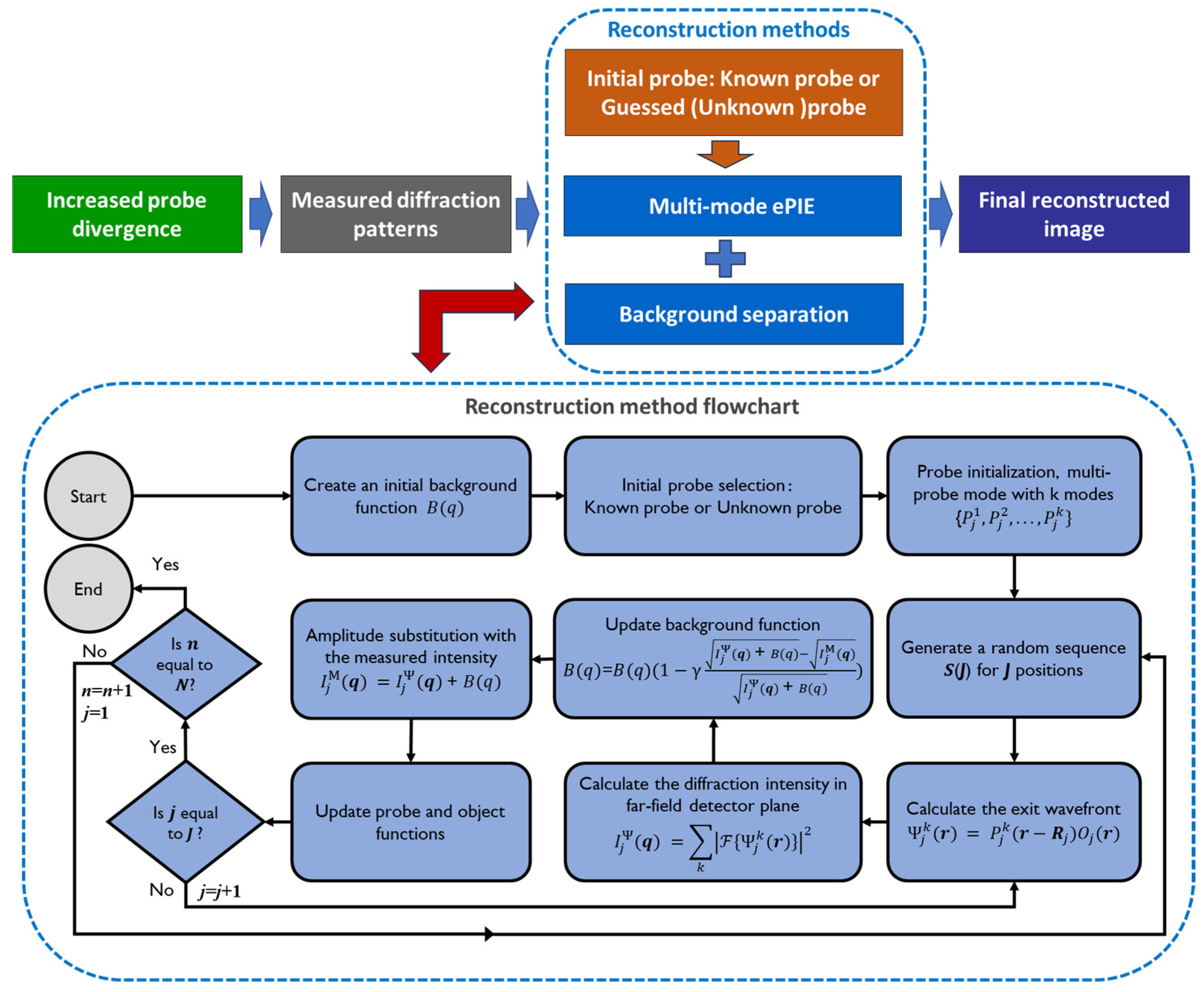
2.1. Partial Recovery of Lost Signals—Using a Known or Near-Accurate Probe

Since both the probe and sample functions are initially unknown, the ptychography algorithm must iteratively update both functions to approach their true values. When signal loss occurs, the missing information in Fourier space will affect both the probe and the object updates, which in turn affects the recovery of lost diffraction signals. This can lead to poor reconstruction quality or even reconstruction failure. For weakly scattering samples, the diffracted signals are usually confined to a small region (the holographic region in the FZP setup) on the detector, making the effect of signal loss more pronounced [19]. For cases with a central beamstop, studies have suggested that an initial reconstruction of the sample profile using data without the beamstop is necessary before reconstructing the long-exposure dataset acquired with the beamstop [24].

Our previous study showed that the correctness of the initial probe function has a significant impact on ptychography reconstruction quality, especially for the illumination generated by an FZP, which has a highly curved wavefront [37]. Therefore, the construction of an appropriate initial probe is essential for a successful reconstruction. For typical experimental setups, a modeled probe derived from the focusing optical element is often used as the initial probe. For example, in an FZP-based experiment, a modeled Fresnel wavefront [37] is used as the initial probe. However, in cases of signal loss, if the initial probe is not close to the true probe, the reconstruction process is more likely to deviate from the true solution direction, leading to significant degradation in reconstruction quality. To address this issue and recover lost signals, we propose the known probe strategy. By performing a quick test with a standard or other easily reconstructed sample (such as a Siemens star, a USAF 1951 resolution board, or other benchmark samples), a reliable probe function can be obtained. By using this function as the initial probe guess, the reconstruction quality of common samples can be improved even in cases of signal loss.

Usually, probe reconstruction is easier than object reconstruction in ptychography. Under signal loss conditions, the pre-experiment for probe measurement may produce a low-quality ptychographic reconstruction. In this case, we can increase the overlap ratio and reduce the scan position number in the pre-experiment on a strong-scattering sample to quickly obtain an accurate probe. If the signal loss is due to the central beamstop, we can obtain a lossless or low-loss dataset by moving out the beamstop or changing to a small beamstop, but the signal-to-noise ratio at high spatial frequencies will be greatly reduced. In this case, we can also improve the probe reconstruction quality by increasing the overlap ratio in the pre-experiment. Therefore, to obtain an accurate probe, a high-overlap small-area ptychographic scan of a strong-scattering sample is necessary prior to the formal imaging experiments.

In the simulations of the known probe approach with an FZP-based setup, the known probe (the ground truth) was used to generate the diffraction patterns and was also used as the initial guess for reconstructions in the known probe case. Conversely, a spherical wave initial probe [37] was used as the initial probe in the unknown probe case. In other words, for the known probe case, both the simulated and initial probes were constructed from the FZP diffraction model [38]; for the unknown probe case, the simulated probe was an FZP model probe, while the initial probe was a spherical wave probe. The initial probes used in these simulations are shown in Figure 3.

In the experimental verifications for the known probe strategy, a probe reconstructed from low-loss or high-overlap data was used as the initial probe for signal loss data reconstruction. For the unknown probe case, an FZP model probe was used as the initial probe.

The known-probe strategy was validated by both simulation and experiment under strip-shaped signal loss conditions, and the conclusion was further generalized to the beamstop-induced signal loss case. For all reconstructions, the reconstruction quality was evaluated by the normalized error in the diffraction patterns, defined as follows:

$$E_{\psi }={\displaystyle \frac{{\sum }_j{{\sum }_k|\sqrt{I_j\left(\mathit{k}\right)}-\left|{\psi }_n(\mathit{k},{\mathit{R}}_{\mathit{j})}\right||}^2}{{\sum }_j{\sum }_k{I}_j\left(\mathit{k}\right)}}$$

(1)

where ${\psi }_n(\mathit{k},{\mathit{R}}_{\mathit{j}})$ represents the exit wave propagated from the reconstructed sample to the frequency domain, and I_j denotes the measured diffraction pattern at the j-th position.

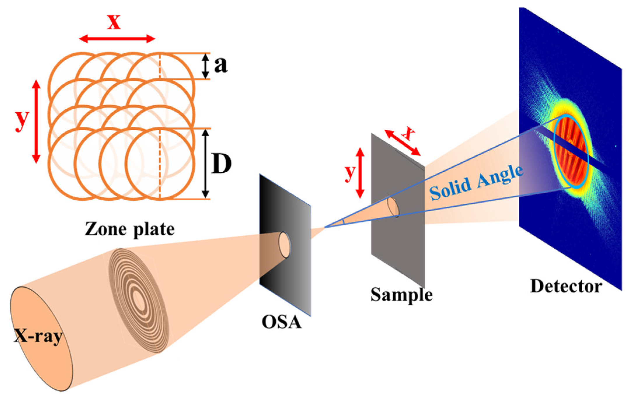
2.2. Suppression of Signal Loss Effects—Probe Divergence

Typically, probe (illumination) divergence, which measures the degree to which a beam spreads outward from its optical axis, can be reliably characterized by the numerical aperture (NA) of the probe. In an FZP-based setup, a large portion or even the majority of the diffraction signals captured by the camera are from the NA of the incident probe, especially for weakly scattering samples. The imaging resolution is often limited by the insufficient scattering capability of the sample. It has been shown that under the presence of high background noise, high-NA probe significantly improves the imaging quality of ptychography [39]. Moreover, increasing the divergence of X-ray beams is usually not easy, and it is also difficult to reduce their divergence without losing flux. In our work, an FZP provides an effective, high-divergence probe, and its divergence can be modified by using FZPs with different outermost zone widths or by using X-rays of different energies.

When the signal loss occurs only in a central beamstop region or an overexposed circular region, the signal loss region can be expressed in terms of an angular span proportional to sinθ (i.e., NA), where θ is half of the divergence angle. However, when the signal loss is no longer confined to a circular region, it cannot simply be described by a two-dimensional angular span. Instead, the solid angle (SA) provides a three-dimensional metric of the angular span of an arbitrary area and is more appropriate for describing arbitrary regions of signal loss as well as the divergence of the probe. In the FZP setup, the SA of the probe, or the divergence of the probe, is defined as the following:

$${\mathrm{S}\mathrm{A}}_{probe}={\int }_A{\displaystyle \frac{\mathrm{d}A}{r^2}}$$

(2)

where dA is the area element, and the integration area (A) is the bright field region on the detector; r is the distance from the focal point to the area element. The SA of the probe is then related to its NA as follows:

$${\mathrm{S}\mathrm{A}}_{probe}\propto {\mathrm{N}\mathrm{A}}^2$$

(3)

The effectiveness of the divergence strategy for suppressing signal loss effects is validated by simulations and experimental data reconstructions. In the simulations, we investigated the reconstruction quality at 7 keV for both strongly and weakly scattering samples under varying probe divergence, sensor gap widths, and scan overlap ratios. When both probe divergence and gap width vary simultaneously, their influence on the ptychography becomes complex. On the one hand, changing the detector gap width also changes the proportion of the signal loss region. On the other hand, the area of diffracted signals on the detector changes (for weakly scattering samples) as the probe divergence changes. To quantitatively study the effect of probe divergence on reconstruction robustness under different signal loss cases, it is necessary to account for the change in the fraction of lost diffraction signals and the change in signal area. After normalizing these factors, the relationship between probe divergence and reconstruction error can finally be established.

Considering the above factors, we defined a quantitative metric to evaluate the relative proportion of lost signals with respect to the SA of diffraction patterns, as shown in Equation (4), where the R_loss (loss ratio) for weakly scattering samples is different from that for strongly scattering samples, as shown in Equation (5).

$${\mathrm{R}\mathrm{a}\mathrm{t}\mathrm{i}\mathrm{o}}_{SA}={(\mathrm{S}\mathrm{A}}_{probe}/{\mathrm{S}\mathrm{A}}_{CCD})/R_{loss}$$

(4)

$$R_{loss}={\displaystyle \frac{{\mathrm{S}\mathrm{A}}_{gap}}{{\mathrm{S}\mathrm{A}}_{diffraction}}}, { \mathrm{S}\mathrm{A}}_{diffraction}=\left\{\begin{array}{c}{\mathrm{S}\mathrm{A}}_{CCD }, \mathrm{S}\mathrm{t}\mathrm{r}\mathrm{o}\mathrm{n}\mathrm{g} \mathrm{s}\mathrm{c}\mathrm{a}\mathrm{t}\mathrm{t}\mathrm{e}\mathrm{r}\mathrm{i}\mathrm{n}\mathrm{g} \\ {\mathrm{S}\mathrm{A}}_{probe}, \mathrm{W}\mathrm{e}\mathrm{a}\mathrm{k} \mathrm{s}\mathrm{c}\mathrm{a}\mathrm{t}\mathrm{t}\mathrm{e}\mathrm{r}\mathrm{i}\mathrm{n}\mathrm{g} \end{array}\right.$$

(5)

Here, we define the signal loss proportion (R_loss) as the ratio of the SA of the signal loss region ${\mathrm{S}\mathrm{A}}_{gap}$ (for both the detector gap and the striped beamstop) to the SA of the entire diffraction signal region ${\mathrm{S}\mathrm{A}}_{diffraction}$. For strongly scattering samples, the diffraction pattern covers almost the entire detector area (Figure 4b). Conversely, for weakly scattering samples, such as cells, the diffraction signal area is nearly identical to the bright field area (the holographic region) formed by the ZP-focused beam (Figure 4a). It should be noted that the definition of the two cases is only to conveniently express the difference in the regional range of the diffraction signal between samples with different scattering capabilities. In actual experiments, the real ${\mathrm{S}\mathrm{A}}_{diffraction}$ can be determined by the maximum measurable diffraction angle. Similarly, for strongly scattering samples, ${\mathrm{S}\mathrm{A}}_{gap}$ is the SA of the entire gap with its length equal to the detector width (Figure 2a), while for weakly scattering samples, ${\mathrm{S}\mathrm{A}}_{gap}$ is the SA of the gap only within the bright field range. In this way, the ${\mathrm{S}\mathrm{A}}_{gap}$ metric can more accurately reflect the signal loss within the effective signal region than the NA of the gap.

After introducing the loss ratio factor R_loss, we further take the influence of the probe divergence (SA_probe/SA_CCD) into account. Finally, we derive a relative SA ratio for signal loss, ${Ratio}_{SA}$ (Equation (4)), which will be referred to in this paper as the “Solid Angle Correction Ratio” (SACR). This metric can compatibly describe the relative signal loss for both strongly and weakly scattering samples.

In the experimental validation, this metric is also used to evaluate the reconstruction quality under signal loss. Since it is impractical to change the FZP in experiments, we adjusted the SACR by changing the sensor gap width in the diffraction pattern, which is roughly equivalent to changing the outermost zone width of the FZP. This allowed us to verify the effectiveness of the suppression strategies.

An overall block diagram is shown in Figure 5 to illustrate the algorithms and methods used in this study. The diffraction data are generated from probes with different divergences, and the initial probe can be a known probe or a guessed model probe. The algorithmic flowchart of ptychographic reconstruction is included in the diagram, showing that the image reconstruction is performed using a multi-mode ePIE algorithm combined with a background separation algorithm [36]. During the iterative reconstruction process, the background function is updated on the Fourier plane for each exposure position using a gradient descent algorithm. The updated background is added to the calculated diffraction intensity and participates in the amplitude substitution step. In the amplitude substitution step, the signal loss region is excluded from the substitution calculation. After a preset iteration number is reached, the results will be output.

3. Results

3.1. Strategy 1: Utilizing a Known Probe

Both simulations and experiments were performed to verify the known probe strategy for partial recovery of lost signals. We compared the reconstruction results of the known probe case with those of the guessed (unknown) probe case under identical experimental parameters and identical signal loss conditions. It is evident that strongly and weakly scattering samples have different diffraction signal distributions (Figure 4). To better illustrate the generality of the signal loss effects, we performed simulations and experiments for both strongly and weakly scattering samples.

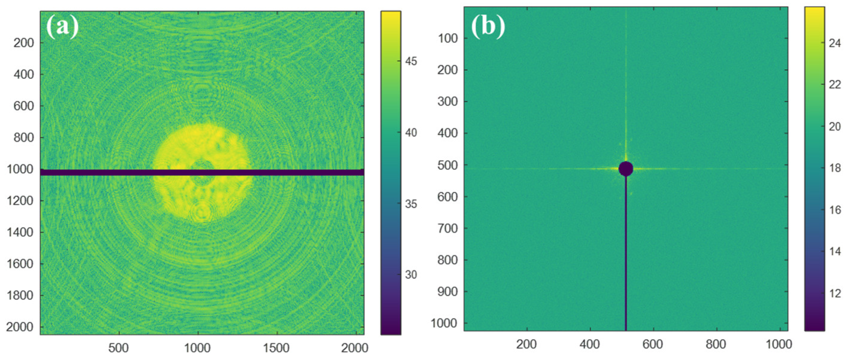
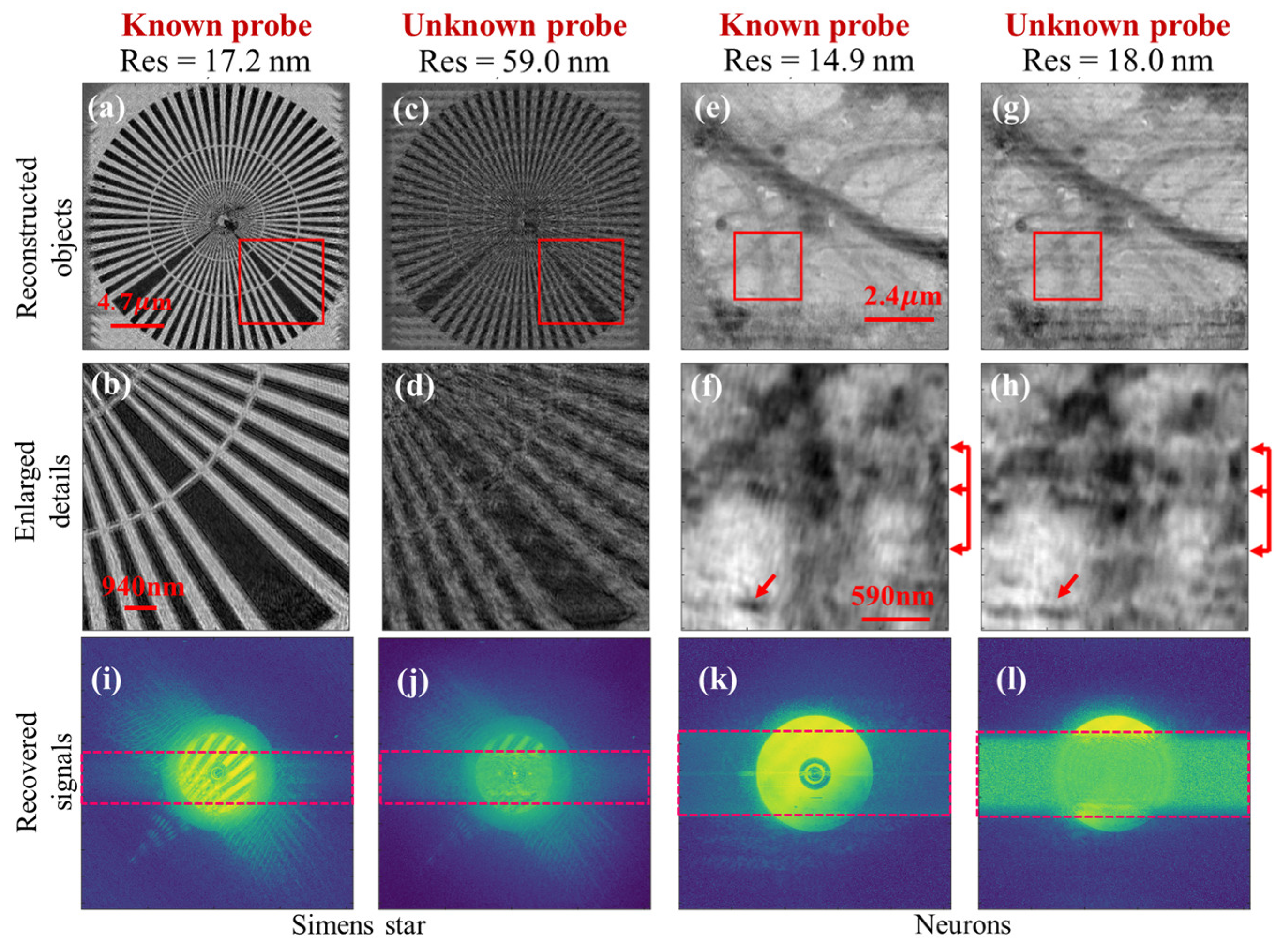
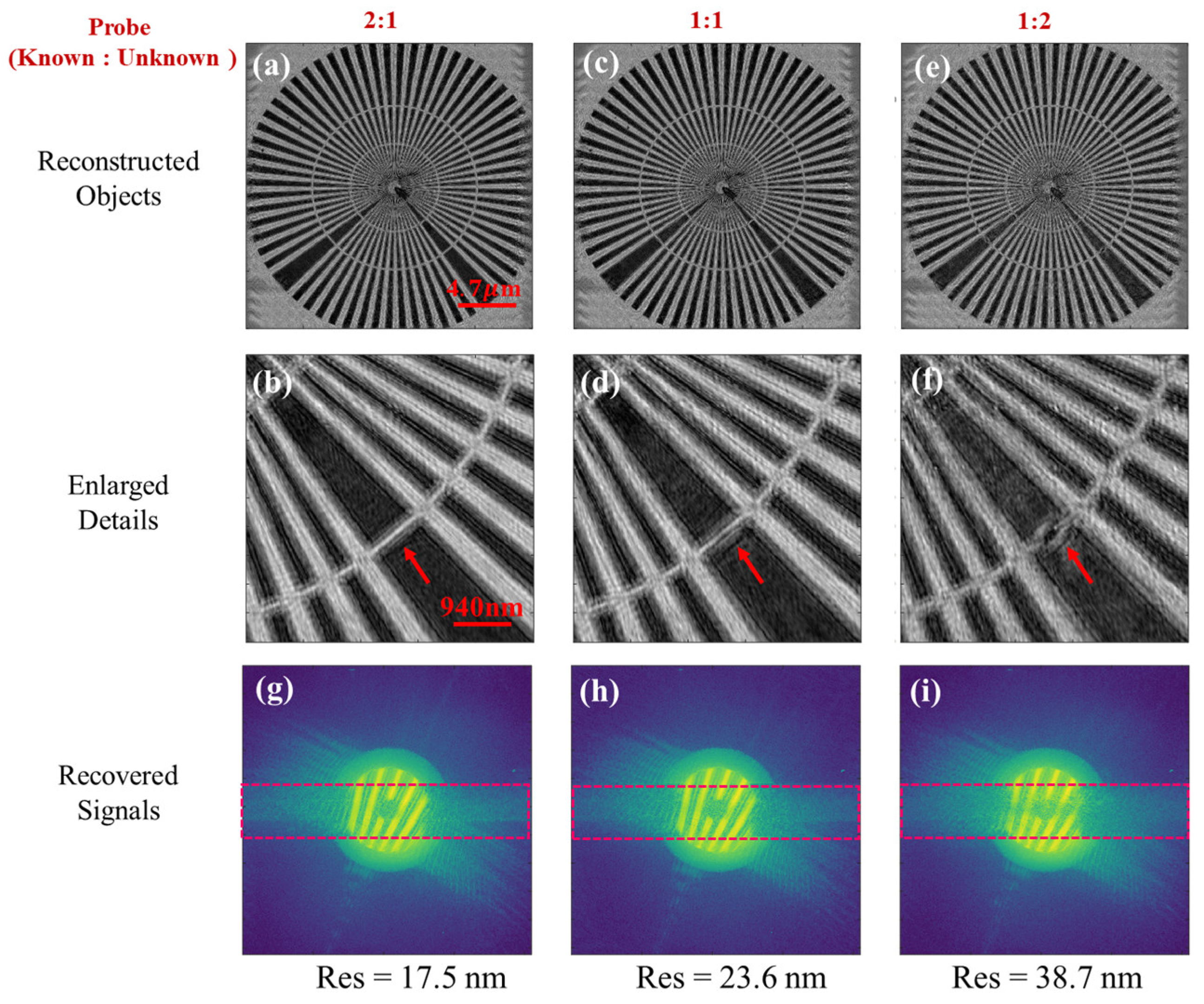
3.1.1. Signal Loss in a Strip-Shaped Gap Region

In the simulations of the strip-shaped signal loss case, the gap region width was set to 50 pixels for both the strongly and weakly scattering samples. The gap length was 1024 pixels, i.e., extending to the edge of the detector. The simulated detector consisted of 1024 × 1024 pixels with a pixel size of 75 μm and was located 2 m downstream of the sample. An FZP with a diameter of 170 μm was used to generate the defocused probe of 2.5 μm diameter with an X-ray photon energy of 7 keV. The outermost zone width of the FZP ranged from 10 nm to 100 nm to produce probes with different divergences. The ptychography scan was performed on an 8 × 9 grid with a step size of 500 nm, resulting in an overlap ratio of 80%. A random noise of 5% average value of the diffraction intensity was added to each diffraction pattern. The sample used in the simulation was constructed from two images. The 1024 × 1024 Goldhill grayscale image was used as the transmittance distribution of the sample with a transmittance range of 0.2~1. The 1024 × 1024 Peppers grayscale image was used as the phase-shift distribution of the sample with a phase-shift range of −π/2~π/2.

In the simulations, we compared the known probe results with the guessed (unknown) probe results for both strongly and weakly scattering samples, and all reconstructions were iterated for 400 steps to ensure reconstruction convergence. The known probe (the ground truth) constructed from the FZP diffraction model and the spherical wave initial probe for the unknown probe case simulations were as they are shown in Figure 3. The simulation results are shown in Figure 6 for both the strongly and weakly scattering samples, where we can see a remarkable improvement in the reconstructed image quality using the known probe as the initial probe over that using a guessed model probe. We also performed simulations with a sample modeled by a uniform material (Au) with a constant complex refractive index, where the contrast came solely from variations in thickness. The simulation results are provided in Part 4 of the Supplementary Materials and show the same conclusion as the results in Figure 6.

The strategy was also validated with experimental data. The verification experiments were performed at the BL08U1A beamline of the Shanghai Synchrotron Radiation Facility (SSRF). In the experiments, a strongly scattering sample (Simens star) and a weakly scattering sample (neurons) were selected for comparative imaging. The X-ray energy was set to 525 eV. The detector used had a 2048 × 2048 pixels array with a pixel size of 11 μm and was located 90 mm downstream of the sample. An FZP with a diameter of 300 μm and an outermost zone width of 30 nm was used to generate the defocused probe of 5 μm diameter for the Simens star and 2.5 μm diameter for the neurons. The ptychography scans were performed on a 20 × 20 grid with a step size of 1 μm for the Simens star and 500 nm for the neuron sample. The total incident doses were 4.42 × 10⁻⁹ J/μm² (2.1 × 10¹⁰ photons) and 1.08 × 10⁻⁸ J/μm² (1.28 × 10¹⁰ photons) for the two experiments, respectively. Both scans have an overlap ratio of 80%. The signal loss gap width ranged from 120 to 400 pixels for the Siemens star, while it ranged from 20 to 370 pixels for the neurons.

The known probe was obtained by reconstructing the diffraction data with a high overlap and low loss ratio and then used as the initial probe for the reconstruction of data with different signal loss sizes (Figure 7a,c). Since the strong scattering and weak scattering experiments were conducted on different days, the shapes of the illumination spots differed significantly. As Figure 7c (weak scattering) shows, the ZP was probably located at the edge of the beam rather than at its center so that one side of the probe appeared weak and cut off. The probe update step in the reconstruction of the known probe case was smaller than that in the unknown probe case. In contrast, for the unknown probe case, reconstructions were performed using an FZP model probe as the initial guess (Figure 7b,d). In iterative reconstruction, the relevant iterative parameter settings differ because the proximity of the probe to the true value is not the same in the known probe condition and the unknown probe condition. We used smaller parameters for probe iteration in the known probe condition and larger parameters in the unknown probe condition. All these parameters were preprocessed before completing the reconstruction to obtain the best reconstruction quality, and all reconstructions were iterated for 400 steps to ensure reconstruction convergence. The width of the gap region was varied to derive the relationship between the reconstruction error and the gap width (Figure 7e,f). It is shown that under signal loss conditions, using a known probe significantly improves the ability of ptychography to recover lost diffraction signals, resulting in a much higher reconstruction quality than using a model initial probe, even for high signal loss ratios. This is further verified by the reconstructed images and the recovered diffraction patterns shown in Figure 8.

From the reconstructed images in Figure 8, we can see that replacing the FZP model probe with the previously reconstructed probe as the initial probe significantly improves the reconstruction quality under signal loss conditions. The resolutions shown in Figure 8 were calculated using the Fourier ring correlation (FRC) method. They are half-period spatial resolutions determined by the half-bit thresholding of the FRC curves. The FRC curves for all the resolution analyses of this paper can be found in the Supplementary Materials. For the strongly scattering (Siemens star) data with a 380-pixel gap width, the periodic grid artifacts in the reconstructed image are greatly suppressed by the known probe input, and the structural details at the stripe edges of the star pattern become much clearer than those of the guessed probe case (Figure 8b,d). For the weakly scattering (neurons) data with a 330-pixel gap width, the improvement by the known probe approach is also remarkable in the reconstructed amplitude images (Figure 8f,h), where the periodic artifacts are markedly suppressed, and the detail fidelity is increased. Figure 8i–l show the lost signal recovery situation after reconstructions, indicating that the known probe approach can recover many more missing signals in the central gap region than the conventional unknown-probe reconstruction.

In addition, to investigate the potential of a partially real probe to facilitate reconstruction with signal loss, an initial probe consisting of a mixture of known and unknown (guessed) probes was employed to reconstruct the Siemens star diffraction data with a gap width of 380 pixels (the same data presented in Figure 8a–d). The known and unknown probes used for the mixture are shown in Figure 7a,b. They were mixed at three different ratios. (1) The ratio of known to unknown probes was 1:2. (2) The ratio of known to unknown probes was 1:1. (3) The ratio of known to unknown probes was 2:1. As can be seen from the reconstructed images in Figure 9, a partially real probe can also improve reconstruction quality under signal loss conditions. As the proportion of the real probe increases, the quality of the reconstructed image improves. This suggests that improving the reconstructed image is possible in practical experiments with signal loss, even if the initial probe is not identical to the real probe but rather similar in some way. The resolutions shown in Figure 9 were calculated using the FRC method, and the corresponding FRC curves are shown in Figure S4 of the Supplementary Materials.

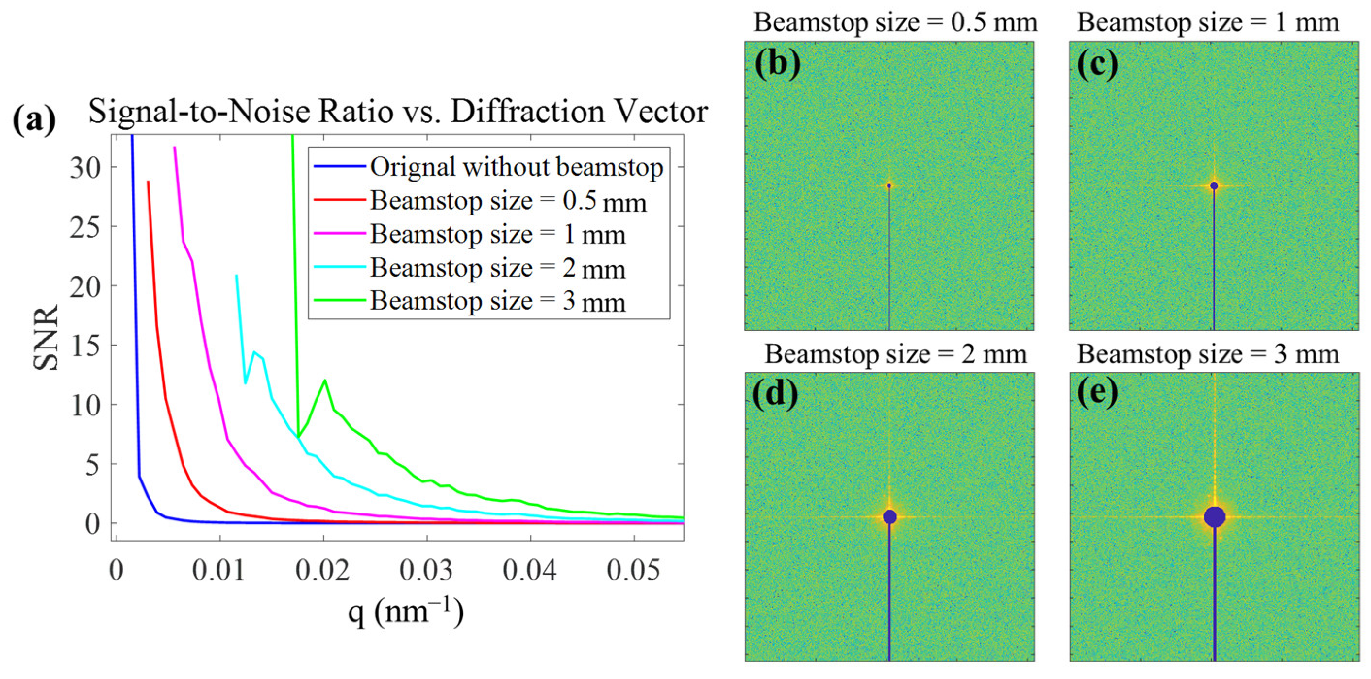
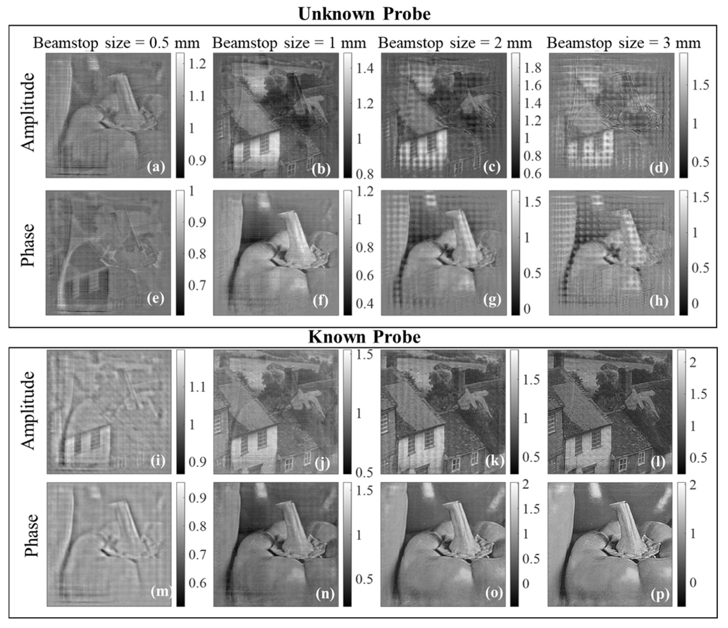
3.1.2. Signal Loss in Central Beamstop Region

A circular or square central beamstop is commonly used in ptychography experiments to block the direct beam and allow long exposures when a KB mirror or aperture is used to constrain the beam. To account for the beamstop-induced signal loss, we performed simulations with a circular beamstop and a KB mirror-focused probe. In the simulations, a square probe of 3.5 um × 3.5 um was chosen with a photon energy of 7 keV, and the scan step size was 600 nm, resulting in a linear overlap ratio of 83%. The beamstop diameters were set to 0.5 mm, 1 mm, 2 mm, and 3 mm, resulting in signal loss ratios of 0.0016, 0.0033, 0.0056, and 0.0087, respectively. To mimic realistic experimental conditions, the exposure times were set according to different beamstop sizes so that the signal intensities matched the dynamic range of the detector, which was $20\times {\mathrm{l}\mathrm{o}\mathrm{g}}_{10}(65532/1) \approx 96.33 \mathrm{d}\mathrm{B}$. In addition, different levels of noise were added to the diffraction patterns at different exposure times. Three types of noise were considered: photon shot noise, dark current noise, and random readout noise. The photon shot noise and the dark current noise are Poisson-distributed and proportional to the exposure time [18]. The scanning process generated 144 diffraction patterns for each case of beamstop size.

The signal-to-noise ratios (SNRs) of the averaged diffraction pattern for different beamstop sizes are plotted as a function of spatial frequency q in Figure 10a. These SNR curves show that increasing the beamstop size allows us to obtain higher SNRs at high spatial frequencies of the diffraction pattern. This improvement suggests that more sample details are captured by the diffraction patterns with a beamstop (Figure 10b–e). However, the loss of low-frequency signals in the central region will make it difficult to converge in the reconstruction. This is confirmed by the reconstructed images shown below.

The reconstructions were performed using both the known probe and unknown (guessed) probe approaches with the initial probes shown in Figure 11. Figure 12a–h show the reconstructed images of the unknown probe case. In this case, a square probe (Figure 11c) was used as the initial guess, and each reconstruction was run for 600 iterations. With a beamstop of 0.5 mm, the overall contour of the sample is well reconstructed, but many details are lost, and significant crosstalk between the phase and amplitude reconstructions is observed (Figure 12a). With a beamstop of 1 mm, most of the details and contour of the sample are well preserved in the reconstruction (Figure 12b). As the beamstop size further increases, strong periodic artifacts dominate the reconstructed images, significantly degrading the reconstruction quality.

In the simulations for the known probe case, the reconstructions were also run for 600 iterations under the same signal loss conditions. The results are shown in Figure 12i–p. We can see that as the beamstop size increases, the reconstructed sample images are consistently improved without encountering the non-convergence problem of reconstruction. Therefore, using a known probe as the initial probe can effectively recover the lost low-frequency signals and solve the non-convergence problem of ptychographic reconstruction when a beamstop is used in experiments.

In ptychography experiments, to achieve high-quality images using the known probe approach or to avoid reconstruction failures due to a beamstop, it is crucial to ensure that the initial probe is either the true probe or close to the true probe. This allows for rapid convergence of the probe solution to the real one during the iterative process. In synchrotron beamlines, the upstream optical components are typically stable enough, and the probe function reconstructed from previous experiments can often be used as a semi-real probe for subsequent reconstructions. If experimental conditions have changed, a quick pre-experiment can be performed on a strongly scattering sample (such as a Siemens star) with a high overlap ratio and few scan points to reconstruct an accurate probe that serves as the initial probe for subsequent large-scale experiments. This approach is particularly useful for studying large-area samples such as IC chips or biological tissues.

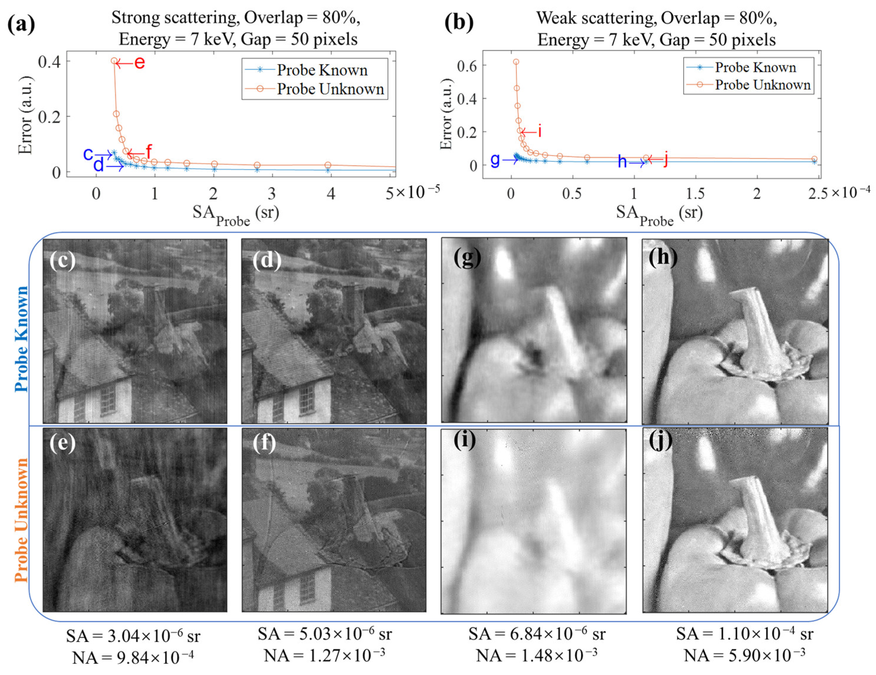
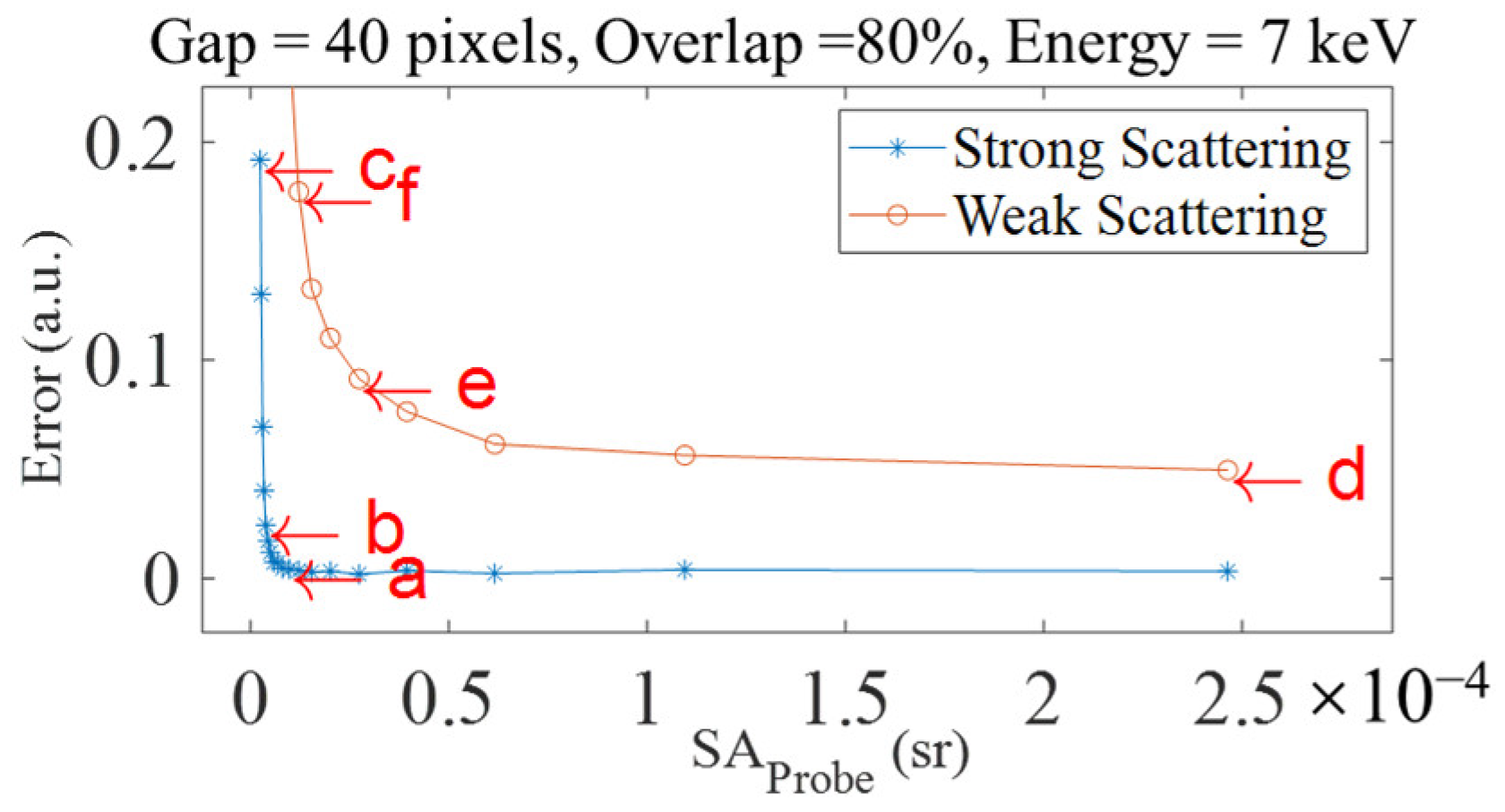
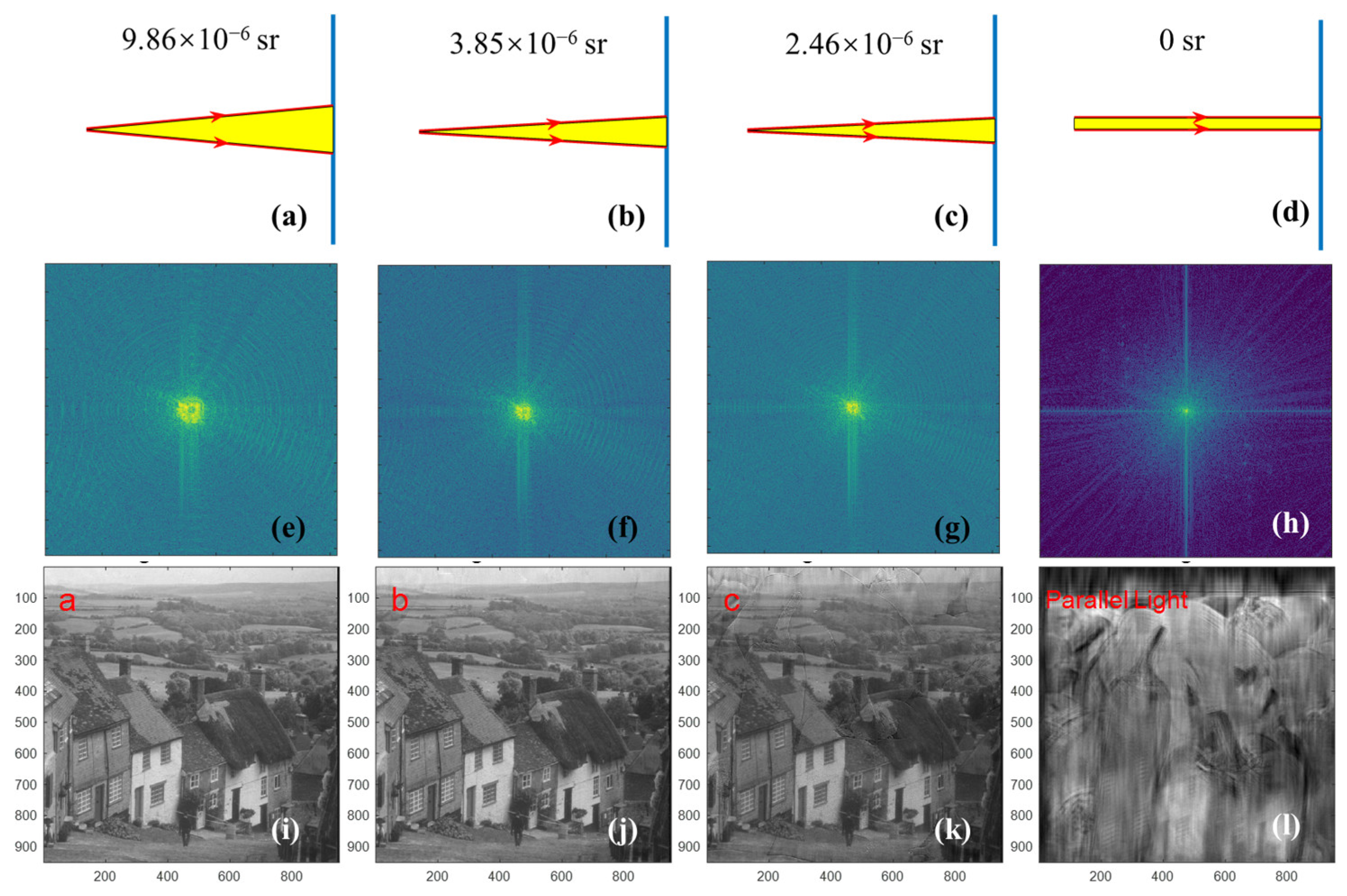
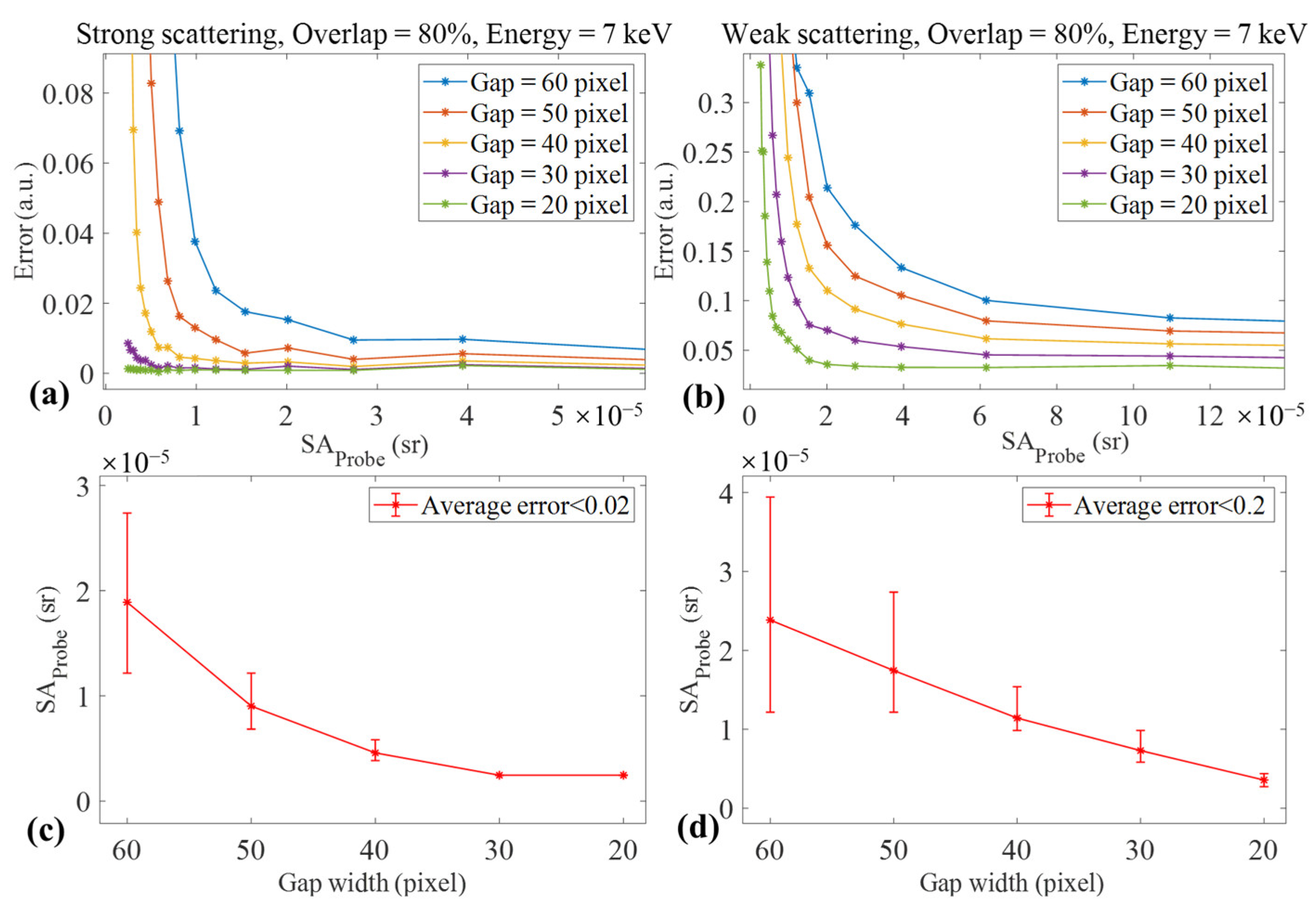
3.2. Strategy 2: Increasing the Divergence of Incident Light

Both simulations and experiments were performed to verify the probe divergence strategy for both strongly and weakly scattering samples. In the simulations, the FZP-modeled probes with different divergences were used to generate diffraction datasets for different signal loss gaps. In the experimental verification, the reconstruction results were compared between different probe divergences implemented by varying the gap width while keeping the FZP fixed. The change in gap width was converted to the change in SACR, which is equivalent to changing the probe divergence.

3.2.1. Simulation Results

The divergence of the incident beam (i.e., the curvature of the wavefront) significantly affects both the quality and stability of CDI reconstructions [1]. In ptychography simulations, we observed that reconstructions of divergent (i.e., focused) beam data have greater tolerance to signal loss than those of parallel beam data, and the image quality from a focused probe is superior to that from a parallel probe. To further verify that probes with higher divergence give ptychography greater robustness to signal loss, we designed simulations for probe divergence effects on reconstruction errors under different signal loss conditions.

In X-ray imaging, focusing elements typically include FZPs, KB mirrors, multilayer mirrors, and compound refractive lenses (CRLs). When studying the effects of probe divergence, the specific focusing element model does not affect the results. In our simulations, X-ray FZPs with different outermost zone widths (ranging from 10 nm to 100 nm) were used to generate probes with different divergences since the NA of an FZP is inversely proportional to its outermost zone width. All reconstructions were iterated for 400 steps to ensure reconstruction convergence. Most of the parameters used here were the same as those used in the simulations in Section 3.1.1, except that the signal loss gap width here ranged from 20 to 60 pixels.

With the fixed width of the striped signal loss region, simulations were performed with a scan overlap ratio of 80%. The relationship between probe SA and reconstruction error is shown in Figure 13. As SA_probe increases, the reconstruction error decreases rapidly, indicating that high probe divergence results in high reconstruction robustness to signal loss. The reconstructed images (Figure 14i–l) provide more direct evidence of this point. A simulation using a parallel-beam (zero divergence) probe was also performed, and its result showed the worst reconstruction quality (Figure 14l), further highlighting the importance of probe divergence for reconstruction under the signal loss condition. The reconstructed images corresponding to points d–f in Figure 13 are provided in Figure S2 in the Supplementary Materials.

To test the generality of the above conclusion for different signal loss regions, we gradually changed the gap width from 20 pixels to 60 pixels and repeated the above simulations. The resulting reconstruction error vs. probe divergence curves are shown in Figure 15a,b, where we can see that the higher the probe divergence, the better the reconstruction quality for all sizes of signal loss areas, further confirming the above conclusion. All reconstructions were iterated for 400 steps. For the same probe SA, the reconstruction error increases as the signal loss area increases.

There is a noticeable difference between the strong and weak scattering cases, i.e., the reconstruction error of the weak scattering sample increases faster than that of the strong scattering sample as the gap width increases from 20 to 60 pixels. This can be seen from the more compact distribution of the error curves for the strong scattering case than for the weak scattering case. Therefore, signal loss in weak scattering cases can cause a more pronounced decrease in reconstruction quality than in strong scattering cases.

Simulations have shown that when the reconstruction error exceeds a certain threshold, the reconstruction quality decreases rapidly. We define the SA corresponding to the error threshold as the critical divergence. Notably, this critical point differs between strong and weak scattering cases. To show intuitively the tolerance of the high probe divergence to the signal loss, we averaged the critical divergences of the probe (the corresponding error threshold is 0.02 for strong scattering and 0.2 for weak scattering) over five repeated computations for each gap width and plotted them in Figure 15c,d. We can see that changing the gap width results in a shift of the critical probe divergence. In the following, we will use the SACR instead of the probe SA as the abscissa to evaluate the signal loss effects. This adjustment brings the critical probe SA values closer together, as shown in Figure 15.

Figure 16 shows the reconstruction errors changing with the SACR for both strongly and weakly scattering samples. After replacing the probe SA with the SACR on the x-axis, the critical points of the SACR (corresponding to the error threshold) for different gap widths are all concentrated within 0~0.2. All curves clearly show that the reconstruction quality is related to the SACR in a more consistent (or compact) way than to the probe SA. Increasing this ratio improves the reconstruction quality under different signal loss conditions.

Examining the definition of SACR (Equation (4)) reveals that this parameter is relevant to the probe divergence, the detector area, the signal loss area, and the fraction of the bright field area in the detector plane. It is known that changing the photon energy while synchronously adjusting the sample-to-detector distance can maintain a constant bright field fraction. Furthermore, our calculation results show that the SACR is independent of the X-ray energy. To better match the experimental conditions, additional simulations based on an FZP setup at 525 eV were performed, showing results consistent with those at 7 keV.

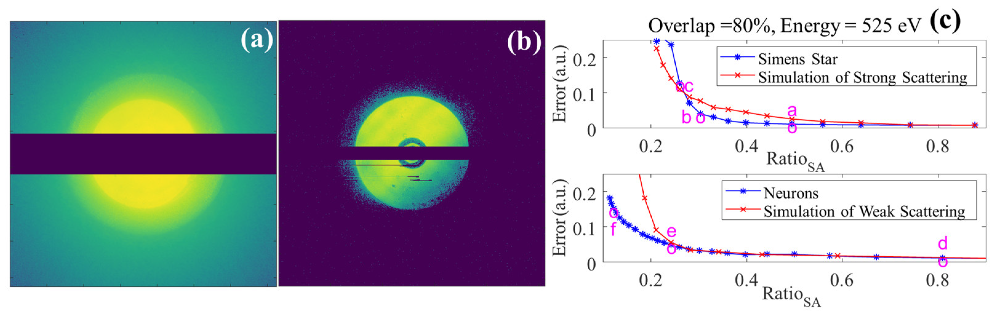
3.2.2. Experimental Results

Direct experimental verification of the probe divergence effect on reconstruction with signal loss requires using a series of FZPs with different focal lengths to obtain different probe divergences. However, this is impractical for real experiments. The above simulations have shown that the reconstruction quality is directly related to the SACR. By changing the gap width while keeping the FZP fixed, i.e., keeping the probe divergence constant, the SACR is also changed. This change is equivalent to inversely adjusting the probe divergence. Therefore, we will experimentally verify the probe divergence strategy by just changing the signal loss gap width.

We performed the verification experiments at the BL08U1A beamline of the SSRF for strategy 2. The experiment parameters used here were the same as those used in the experiments in Section 3.1.1, and the same samples (Simens star and neurons) were also imaged here. All reconstructions were iterated for 400 steps to ensure reconstruction convergence.

By displaying the pattern on a logarithmic scale, the actual extent of the diffraction pattern can be observed. The average diffraction pattern is calculated from the dataset and shown in Figure 17a,b. We can see that the diffraction pattern of the weakly scattering sample (Figure 17a) is mainly concentrated in the bright field region on the detector. In contrast, the diffraction pattern of the strongly scattering sample (Figure 17b) spans the entire detector area.

The reconstruction errors of the experimental data for the Siemens star and neuron samples are shown as blue curves in Figure 17c. For comparison, simulations with the same parameters as the experiments were also performed, and their reconstruction errors are shown as red curves. Several typical reconstructed images of the experimental data with different SACRs are shown in Figure 18. Their corresponding SACRs are labeled with the letters a–f in Figure 17c.

From the two sets of experimental results, it can be seen that both strongly and weakly scattering samples are better reconstructed at higher SACRs (higher probe divergences). When the SACR is above 0.3 (corresponding to a gap width below 320 pixels), the reconstruction quality decreases slowly with decreasing SACR, but when the SACR decreases to below 0.3, the reconstruction quality deteriorates rapidly. The resolutions shown in Figure 18 are calculated using the FRC method. They also confirm that the higher the SACR or probe divergence, the better the reconstructed images.

4. Discussion

By increasing the divergence of the incident probe, the quality of the reconstructed image can be improved under signal loss conditions. In the introduction section, we mentioned that in the case of signal loss due to a central beamstop, a previous study showed that the reconstruction quality degrades abruptly when the ratio of the beamstop NA to the probe NA is greater than 1. To investigate more general cases, such as stripe-shaped signal loss, we used the solid angle correction ratio (SACR) to quantitatively describe the relative signal loss, and this parameter is a modified ratio of the probe SA to the signal loss SA. The critical point for rapid degradation of reconstruction quality with respect to the SACR is different for weak scattering and strong scattering cases. In the case of strong scattering, the SACR is the ratio of the probe SA to the gap SA, and the critical value is about 0.25 for both simulations and experiments. In the case of weak scattering, the SACR is further modified by the ratio of probe SA to detector SA, and the critical value is about 0.2 in our experiments.

The known probe method has previously been used to reconstruct weakly scattered samples as it speeded up the convergence rate and reduced artifacts in the reconstructed image. There has been no investigation on the application of this method to compensate for the signal loss in ptychography. Our study focuses on the recovery of lost diffraction signals using the known probe method and verifies that this method can significantly improve the reconstruction quality in the case of signal loss.

Among the two methods we presented, the known probe method is found to be suitable for recovering lost signals in a variety of signal loss situations, including central beamstop, detector gap, and oversaturation due to long exposures. Meanwhile, this method is found to be suitable for both high divergence probe (FZP focused spot) and low divergence probe (KB mirror or small aperture source) cases with signal loss. The experimental results of the increased probe divergence method showed that when signal loss is unavoidable in the experiment, the choice of a high divergence illumination is advantageous for the subsequent reconstruction of the sample.

Furthermore, we observed the synergistic effect of the two presented methods. In the simulations of the known probe method, we have verified that this method further improves the reconstruction quality compared to the guessed initial probe method as the probe divergence increases, as shown in Figure 6. Meanwhile, the relationship between the reconstruction error and the probe divergence for the known probe method alone (Figure 19a) shows that the reconstruction error decreases rapidly as the probe divergence increases. This indicates that the known probe method and the probe divergence method have a synergistic effect in suppressing the signal loss impacts. In addition, in the experimental results for the known probe strategy, the reconstruction results were presented under both known probe and unknown probe conditions with different gap widths. When investigating the effect of probe divergence on reconstruction quality, the gap width change can be equated to the probe divergence inverse change. Therefore, the experimental results with different gap widths under the known probe condition can be seen as an experimental result of the synergistic effect of the two methods. As shown in Figure 19b for the experimental result, when the gap width increases or the probe divergence (or the SACR) decreases, the reconstruction error rapidly increases in the interval between d and c, indicating a critical behavior. The experimental result comparison of the synergistic effect of the two methods with the unknown probe case can be seen in Figure 7e,f.

5. Conclusions

In this study, we presented two approaches, using a known probe and increasing the probe divergence, to compensate for the effects of signal loss. We investigated the effects of several factors, including initial probe selection, probe divergence, scan overlap ratio, and signal area ratio, on ptychography reconstruction quality in the presence of signal loss due to a detector gap or a central beamstop. Through simulations and experimental reconstructions, we found that when a known probe is used as the initial probe, the lost signals can be largely recovered in both strong and weak scattering cases. Even in the case of severe signal loss, the known probe reconstruction can remain of high quality. It was also found that higher probe divergence can make ptychography more robust in terms of signal loss and effectively mitigate the degradation of reconstruction quality due to missed signals. This suggests that using a high-divergence probe can suppress the signal loss effects and improve reconstruction quality. Since the two strategies do not require additional scans, they reduce both experimental and reconstruction complexity compared to previous strategies.

This study highlights the importance of optimizing experimental parameters, such as probe divergence and overlap ratio, in suppressing the effects of signal loss. More importantly, the proposed known-probe approach provides a practical solution for improving reconstruction quality in cases of significant signal loss. By conducting a pre-experiment with a standard sample to obtain a realistic probe, the known-probe approach can serve as a valuable tool for high-quality imaging of large or complicated samples, such as biological tissues or IC chips.

In addition, as deep learning methods continue to evolve for ptychographic imaging, the prediction of lost signals using these methods will be an important developing direction [40]. For instance, deep-learning-based inpainting techniques have been suggested for recovering missing information in X-ray scattering images [41]. However, it is more difficult to obtain direct predictions for diffraction images of amorphous materials in ptychography. Nevertheless, unsupervised modeling of physical constraints provides new ideas for development in this direction [42].

This study mainly focuses on the signal loss due to a central gap or central beamstop and does not investigate the case where the central signals are preserved with the signal loss occurring at the periphery. However, the conclusion of this study may be applicable to the cases of peripheral signal loss. In future work, we will investigate the effect of signal loss in more complex spatial distributions.

References

1. Bosch, C.; Aidukas, T.; Holler, M.; Pacureanu, A.; Müller, E.; Peddie, C.J.; Zhang, Y.; Cook, P.; Collinson, L.; Bunk, O.; et al. Non-Destructive X-Ray Tomography of Brain Tissue Ultrastructure. bioRxiv 2024. [Google Scholar] [CrossRef]
2. Csernica, P.M.; Kalirai, S.S.; Gent, W.E.; Lim, K.; Yu, Y.-S.; Liu, Y.; Ahn, S.-J.; Kaeli, E.; Xu, X.; Stone, K.H.; et al. Persistent and Partially Mobile Oxygen Vacancies in Li-Rich Layered Oxides. Nat. Energy 2021, 6, 642–652. [Google Scholar] [CrossRef]
3. Deng, J.; Lo, Y.H.; Gallagher-Jones, M.; Chen, S.; Pryor, A.; Jin, Q.; Hong, Y.P.; Nashed, Y.S.G.; Vogt, S.; Miao, J.; et al. Correlative 3D X-Ray Fluorescence and Ptychographic Tomography of Frozen-Hydrated Green Algae. Sci. Adv. 2018, 4, eaau4548. [Google Scholar] [CrossRef] [PubMed]
4. Dierolf, M.; Menzel, A.; Thibault, P.; Schneider, P.; Kewish, C.M.; Wepf, R.; Bunk, O.; Pfeiffer, F. Ptychographic X-Ray Computed Tomography at the Nanoscale. Nature 2010, 467, 436–439. [Google Scholar] [CrossRef]
5. Donnelly, C.; Guizar-Sicairos, M.; Scagnoli, V.; Gliga, S.; Holler, M.; Raabe, J.; Heyderman, L.J. Three-Dimensional Magnetization Structures Revealed with X-Ray Vector Nanotomography. Nature 2017, 547, 328–331. [Google Scholar] [CrossRef]
6. Lo, Y.H.; Zhou, J.; Rana, A.; Morrill, D.; Gentry, C.; Enders, B.; Yu, Y.-S.; Sun, C.-Y.; Shapiro, D.A.; Falcone, R.W.; et al. X-Ray Linear Dichroic Ptychography. Proc. Natl. Acad. Sci. USA 2021, 118, e2019068118. [Google Scholar] [CrossRef]
7. Guizar-Sicairos, M.; Johnson, I.; Diaz, A.; Holler, M.; Karvinen, P.; Stadler, H.-C.; Dinapoli, R.; Bunk, O.; Menzel, A. High-Throughput Ptychography Using Eiger: Scanning X-Ray Nano-Imaging of Extended Regions. Opt. Express 2014, 22, 14859–14870. [Google Scholar] [CrossRef] [PubMed]
8. Jørgensen, P.S.; Besley, L.; Slyamov, A.M.; Diaz, A.; Guizar-Sicairos, M.; Odstrčil, M.; Holler, M.; Silvestre, C.; Chang, B.; Detlefs, C.; et al. Hard X-Ray Grazing-Incidence Ptychography: Large Field-of-View Nanostructure Imaging with Ultra-High Surface Sensitivity. Optica 2024, 11, 197. [Google Scholar] [CrossRef]
9. Holler, M.; Diaz, A.; Guizar-Sicairos, M.; Karvinen, P.; Färm, E.; Härkönen, E.; Ritala, M.; Menzel, A.; Raabe, J.; Bunk, O. X-Ray Ptychographic Computed Tomography at 16 Nm Isotropic 3D Resolution. Sci. Rep. 2014, 4, 3857. [Google Scholar] [CrossRef]
10. Deng, J.; Preissner, C.; Klug, J.A.; Mashrafi, S.; Roehrig, C.; Jiang, Y.; Yao, Y.; Wojcik, M.; Wyman, M.D.; Vine, D.; et al. The Velociprobe: An Ultrafast Hard X-Ray Nanoprobe for High-Resolution Ptychographic Imaging. Rev. Sci. Instrum. 2019, 90, 083701. [Google Scholar] [CrossRef]
11. Yao, Y.; Jiang, Y.; Klug, J.A.; Wojcik, M.; Maxey, E.R.; Sirica, N.S.; Roehrig, C.; Cai, Z.; Vogt, S.; Lai, B.; et al. Multi-Beam X-Ray Ptychography for High-Throughput Coherent Diffraction Imaging. Sci. Rep. 2020, 10, 19550. [Google Scholar] [CrossRef] [PubMed]
12. Rana, A.; Liao, C.-T.; Iacocca, E.; Zou, J.; Pham, M.; Lu, X.; Subramanian, E.-E.C.; Lo, Y.H.; Ryan, S.A.; Bevis, C.S.; et al. Three-Dimensional Topological Magnetic Monopoles and Their Interactions in a Ferromagnetic Meta-Lattice. Nat. Nanotechnol. 2023, 18, 227–232. [Google Scholar] [CrossRef]
13. Deng, J.; Hong, Y.P.; Chen, S.; Nashed, Y.S.G.; Peterka, T.; Levi, A.J.F.; Damoulakis, J.; Saha, S.; Eiles, T.; Jacobsen, C. Nanoscale X-Ray Imaging of Circuit Features without Wafer Etching. Phys. Rev. B 2017, 95, 104111. [Google Scholar] [CrossRef] [PubMed]
14. Gorkhover, T.; Rupp, D. Microchip Minutiae Imaged Using X-Ray Bursts. Nature 2024, 632, 36–38. [Google Scholar] [CrossRef]
15. Miao, J. Computational Microscopy with Coherent Diffractive Imaging and Ptychography. Nature 2025, 637, 281–295. [Google Scholar] [CrossRef] [PubMed]
16. Reinhardt, J.; Hoppe, R.; Hofmann, G.; Damsgaard, C.D.; Patommel, J.; Baumbach, C.; Baier, S.; Rochet, A.; Grunwaldt, J.-D.; Falkenberg, G.; et al. Beamstop-Based Low-Background Ptychography to Image Weakly Scattering Objects. Ultramicroscopy 2017, 173, 52–57. [Google Scholar] [CrossRef]
17. Schropp, A.; Schroer, C.G. Dose Requirements for Resolving a given Feature in an Object by Coherent X-Ray Diffraction Imaging. New J. Phys. 2010, 12, 035016. [Google Scholar] [CrossRef]
18. Granados, M.; Ajdin, B.; Wand, M.; Theobalt, C.; Seidel, H.-P.; Lensch, H.P.A. Optimal HDR Reconstruction with Linear Digital Cameras. In Proceedings of the 2010 IEEE Computer Society Conference on Computer Vision and Pattern Recognition, San Francisco, CA, USA, 13–18 June 2010; pp. 215–222. [Google Scholar]
19. Dierolf, M.; Thibault, P.; Menzel, A.; Kewish, C.M.; Jefimovs, K.; Schlichting, I.; König, K.V.; Bunk, O.; Pfeiffer, F. Ptychographic Coherent Diffractive Imaging of Weakly Scattering Specimens. New J. Phys. 2010, 12, 035017. [Google Scholar] [CrossRef]
20. Henrich, B.; Bergamaschi, A.; Broennimann, C.; Dinapoli, R.; Eikenberry, E.F.; Johnson, I.; Kobas, M.; Kraft, P.; Mozzanica, A.; Schmitt, B. PILATUS: A Single Photon Counting Pixel Detector for X-Ray Applications. Nucl. Instrum. Methods Phys. Res. Sect. A Accel. Spectrometers Detect. Assoc. Equip. 2009, 607, 247–249. [Google Scholar] [CrossRef]
21. Shukla, A.; Wright, J.; Henningsson, A.; Stieglitz, H.; Colegrove, E.; Besley, L.; Baur, C.; De Angelis, S.; Stuckelberger, M.; Poulsen, H.F.; et al. Grain Boundary Strain Localization in a CdTe Solar Cell Revealed by Scanning 3D X-Ray Diffraction Microscopy. J. Mater. Chem. A 2024, 12, 16793–16802. [Google Scholar] [CrossRef]
22. Takahashi, Y.; Suzuki, A.; Furutaku, S.; Yamauchi, K.; Kohmura, Y.; Ishikawa, T. High-Resolution and High-Sensitivity Phase-Contrast Imaging by Focused Hard x-Ray Ptychography with a Spatial Filter. Appl. Phys. Lett. 2013, 102, 094102. [Google Scholar] [CrossRef]
23. Thibault, P.; Dierolf, M.; Menzel, A.; Bunk, O.; David, C.; Pfeiffer, F. High-Resolution Scanning X-Ray Diffraction Microscopy. Science 2008, 321, 379–382. [Google Scholar] [CrossRef]
24. Rose, M.; Dzhigaev, D.; Senkbeil, T.; von Gundlach, A.R.; Stuhr, S.; Rumancev, C.; Besedin, I.; Skopintsev, P.; Viefhaus, J.; Rosenhahn, A.; et al. High-Dynamic-Range Water Window Ptychography. J. Phys. Conf. Ser. 2017, 849, 012027. [Google Scholar] [CrossRef]
25. Takahashi, Y.; Suzuki, A.; Zettsu, N.; Kohmura, Y.; Yamauchi, K.; Ishikawa, T. Multiscale Element Mapping of Buried Structures by Ptychographic X-Ray Diffraction Microscopy Using Anomalous Scattering. Appl. Phys. Lett. 2011, 99, 131905. [Google Scholar] [CrossRef]
26. Guizar-Sicairos, M.; Holler, M.; Diaz, A.; Vila-Comamala, J.; Bunk, O.; Menzel, A. Role of the Illumination Spatial-Frequency Spectrum for Ptychography. Phys. Rev. B 2012, 86, 100103. [Google Scholar] [CrossRef]
27. Holler, M.; Guizar-Sicairos, M.; Tsai, E.H.R.; Dinapoli, R.; Müller, E.; Bunk, O.; Raabe, J.; Aeppli, G. High-Resolution Non-Destructive Three-Dimensional Imaging of Integrated Circuits. Nature 2017, 543, 402–406. [Google Scholar] [CrossRef]
28. Vila-Comamala, J.; Diaz, A.; Guizar-Sicairos, M.; Mantion, A.; Kewish, C.M.; Menzel, A.; Bunk, O.; David, C. Characterization of High-Resolution Diffractive X-Ray Optics by Ptychographic Coherent Diffractive Imaging. Opt. Express 2011, 19, 21333. [Google Scholar] [CrossRef]
29. Shapiro, D.A.; Yu, Y.-S.; Tyliszczak, T.; Cabana, J.; Celestre, R.; Chao, W.; Kaznatcheev, K.; Kilcoyne, A.L.D.; Maia, F.; Marchesini, S.; et al. Chemical Composition Mapping with Nanometre Resolution by Soft X-Ray Microscopy. Nat. Photon 2014, 8, 765–769. [Google Scholar] [CrossRef]
30. Aidukas, T.; Phillips, N.W.; Diaz, A.; Poghosyan, E.; Müller, E.; Levi, A.F.J.; Aeppli, G.; Guizar-Sicairos, M.; Holler, M. High-Performance 4-nm-Resolution X-Ray Tomography Using Burst Ptychography. Nature 2024, 632, 81–88. [Google Scholar] [CrossRef]
31. Atakul-Özdemir, A.; Warren, X.; Martin, P.G.; Guizar-Sicairos, M.; Holler, M.; Marone, F.; Martínez-Pérez, C.; Donoghue, P.C.J. X-Ray Nanotomography and Electron Backscatter Diffraction Demonstrate the Crystalline, Heterogeneous and Impermeable Nature of Conodont White Matter. R. Soc. Open Sci. 2021, 8, 202013. [Google Scholar] [CrossRef]
32. Jiang, Y.; Deng, J.; Yao, Y.; Klug, J.A.; Mashrafi, S.; Roehrig, C.; Preissner, C.; Marin, F.S.; Cai, Z.; Lai, B.; et al. Achieving High Spatial Resolution in a Large Field-of-View Using Lensless X-Ray Imaging. Appl. Phys. Lett. 2021, 119, 124101. [Google Scholar] [CrossRef]
33. Weber, C.C.; De Angelis, S.; Meinert, R.; Appel, C.; Holler, M.; Guizar-Sicairos, M.; Gubler, L.; Büchi, F.N. Microporous Transport Layers Facilitating Low Iridium Loadings in Polymer Electrolyte Water Electrolysis. EES. Catal. 2024, 2, 585–602. [Google Scholar] [CrossRef]
34. Dejkameh, A.; Nebling, R.; Locans, U.; Kim, H.-S.; Mochi, I.; Ekinci, Y. Recovery of Spatial Frequencies in Coherent Diffraction Imaging in the Presence of a Central Obscuration. Ultramicroscopy 2024, 258, 113912. [Google Scholar] [CrossRef]
35. Thibault, P.; Menzel, A. Reconstructing state mixtures from diffraction measurements. Nature 2023, 494, 68–71. [Google Scholar] [CrossRef] [PubMed]
36. Xing, Z.; Xu, Z.; Sun, T.; Zhang, X.; Tai, R. Research on Signal-Noise Separation Algorithm of Ptychography. Acta Opt. Sin. 2021, 41, 2234001. [Google Scholar] [CrossRef]
37. Qin, Z.; Xu, Z.; Li, R.; Liu, H.; Liu, S.; Wen, Q.; Chen, X.; Zhang, X.; Tai, R. Initial Probe Function Construction in Ptychography Based on Zone-Plate Optics. Appl. Opt. 2023, 62, 3542. [Google Scholar] [CrossRef]
38. Quiney, H.M.; Peele, A.G.; Cai, Z.; Paterson, D.; Nugent, K.A. Diffractive Imaging of Highly Focused X-Ray Fields. Nat. Phys. 2006, 2, 101–104. [Google Scholar] [CrossRef]
39. Zhang, W.; Dresselhaus, J.L.; Fleckenstein, H.; Prasciolu, M.; Zakharova, M.; Ivanov, N.; Li, C.; Yefanov, O.; Li, T.; Egorov, D.; et al. Fast and Efficient Hard X-Ray Projection Imaging below 10 nm Resolution. Opt. Express 2024, 32, 30879. [Google Scholar] [CrossRef]
40. Cherukara, M.J.; Zhou, T.; Nashed, Y.; Enfedaque, P.; Hexemer, A.; Harder, R.J.; Holt, M.V. Real-Time Sparse-Sampled Ptychographic Imaging Through Deep Neural Networks. arXiv 2020, arXiv:2004.08247. [Google Scholar] [CrossRef]
41. Chavez, T.; Roberts, E.J.; Zwart, P.H.; Hexemer, A. A Comparison of Deep-Learning-Based Inpainting Techniques for Experimental X-Ray Scattering. J. Appl. Crystallogr. 2022, 55, 1277–1288. [Google Scholar] [CrossRef]
42. Hoidn, O.; Mishra, A.A.; Mehta, A. Physics Constrained Unsupervised Deep Learning for Rapid, High Resolution Scanning Coherent Diffraction Reconstruction. Sci. Rep. 2023, 13, 22789. [Google Scholar] [CrossRef] [PubMed]
Figure 1. Experimental setup for ptychography. The probe divergence is represented by the solid angle of the bright field of the FZP-focused illumination. The inset in the upper left corner shows the scanning scheme. Here, a is the scan step size, D is the spot diameter, and the linear overlap ratio is 1 − a/D.
Photonics 12 00636 g001
Figure 2. Illustration of two representative types of signal loss regions in the far-field diffraction patterns. (a) Striped gap; (b) central beamstop.
Photonics 12 00636 g002
Figure 3. Probe models used in the simulations. (a,b) The spherical wave model probe, which was used as the initial probe for reconstructions in the unknown probe case. (c,d) The FZP model probe, which was used as the probe to generate diffraction data and as the initial probe for reconstructions in the known probe case.
Photonics 12 00636 g003
Figure 4. Typical simulated diffraction patterns on a logarithmic scale for a weakly scattering sample (a) and a strongly scattering sample (b). The weak scattering pattern is distributed within the bright field, while the strong scattering pattern covers the entire detector area. In weak scattering patterns, the diffraction signals outside the bright field were set as the mean background value of the detector edges.
Photonics 12 00636 g004
Figure 5. The algorithms and methods used in compensating for lost signals. In the reconstruction, we adopted a multi-mode ePIE algorithm combined with a background separation algorithm. In the above framework, the diffraction data with increased probe divergence are input into the reconstruction algorithm. Meanwhile, the algorithmic flowchart is shown in the block below, where the initial probe can be a known probe or an unknown (guessed) probe.
Photonics 12 00636 g005
Figure 6. The simulation results for strategy 1. (a,cf) The results for a strongly scattering sample with a signal loss gap of 50-pixel width. (b,gj) The results for a weakly scattering sample with the same signal loss gap. (a,b) The reconstruction quality as a function of probe divergence for the known (blue curves) and unknown (orange curves) probe cases. The labeled points correspond to the reconstructed images. (cf) Reconstructed amplitude images of the strongly scattering sample using the known probe approach (c,d) or a guessed initial probe (e,f) with different probe SAs. (gj) Reconstructed phase images of the weakly scattering sample using the known probe approach (g,h) or a guessed initial probe (i,j) with different probe SAs. The probe divergence for each column of reconstructed images is labeled at the bottom.
Photonics 12 00636 g006
Figure 7. Initial probes (ad) used in the experiment data reconstructions for strategy 1 with their reconstruction errors (e,f) as a function of gap width. (a,b) The known and guessed (unknown) initial probes (FZP model probe), respectively, for the strong scattering data reconstruction. (c,d) The known and guessed initial probes for the weak scattering data reconstruction. (e,f) show reconstruction errors for the strongly and weakly scattering samples, respectively, where points a, b, c, and d correspond to the reconstructed images in Figure 8a,c,e,g, respectively. The gap width in (e) ranges from 120 to 400 pixels, while in (f), it ranges from 20 to 370 pixels.
Photonics 12 00636 g007
Figure 8. Comparison of experimental reconstructed images for strategy 1. (ad) The reconstructed Siemens star images with a known probe (a,b) or a guessed probe (c,d), where (b,d) are the enlarged red-box areas in (a,c), respectively. The gap width for this experiment is 380 pixels. (eh) The reconstructed images for the neurons with a known probe (e,f) or a guessed probe (g,h), where (f,h) are the enlarged red-box areas in (e,g), respectively. The gap width for this experiment is 330 pixels. The red arrows in (f,h) highlight the differences between the two images. (il) The recovered diffraction patterns during the four reconstructions. The “Res” on the top of the figure means resolution. The red dashed boxes in (il) denote the signal recovery (or loss) areas.
Photonics 12 00636 g008
Figure 9. Comparison of experimental reconstructed images using partially real probes. The gap width for this experimental data is 380 pixels, which is the same as for Figure 8a–d. (af) Reconstructed Siemens star images with a 2:1 mixture of known and unknown (guessed) probes (a,b), a 1:1 mixture (c,d), and a 1:2 mixture (e,f). The red arrows in (b,d,f) highlight the differences between the three images. (gi) The recovered diffraction patterns during the three reconstructions. The “Res” under the figure means resolution. The red dashed boxes in (gi) denote the signal recovery (or loss) areas.
Photonics 12 00636 g009
Figure 10. Signal distributions in central beamstop simulations. (a) The SNRs of the averaged diffraction pattern as a function of the diffraction vector q for different beamstop sizes. The curves show that larger beamstops result in higher SNRs at high spatial frequencies. (be) Simulated diffraction patterns with beamstops of 0.5 mm, 1 mm, 2 mm, and 3 mm diameter, respectively.
Photonics 12 00636 g010
Figure 11. Amplitudes and phases of the known probe (a,b) and initial guess for the unknown probe (c,d).
Photonics 12 00636 g011
Figure 12. (ah) Reconstructed amplitude and phase images with a guessed initial probe for different beamstop sizes. (ip) Reconstructed amplitude and phase images with a known probe for different beamstop sizes.
Photonics 12 00636 g012
Figure 13. Reconstruction errors as a function of probe divergence (SAprobe) for the same signal loss gap width (40 pixels) in the simulations for strategy 2. The results show that increasing the probe divergence improves the reconstruction quality. The reconstructed images for points a–c are shown in Figure 14i–k, respectively, while the images for points d–f are provided in Figure S2a–c, respectively, in the Supplementary Materials.
Photonics 12 00636 g013
Figure 14. Simulation results of different probe divergences. (ad) Illustrations of incident probes with differently divergent SAs used in the simulation. (eh) The corresponding diffraction patterns at the detector plane, where the central pattern shrinks with decreasing divergence. (il) A comparison of reconstructed amplitude images for different probe SAs, where the parallel-beam result has the lowest reconstruction quality.
Photonics 12 00636 g014
Figure 15. Simulation results of probe SA effects for different gap widths. (a,b) The reconstruction error vs. probe SA under different gap widths. (c,d) The critical probe SAs changing with the gap width. The results show that a probe of higher divergence can tolerate a larger signal loss region.
Photonics 12 00636 g015
Figure 16. Simulated reconstruction error vs. SACR at different gap widths. (a) Strong scattering results. (b) Weak scattering results. The curves show a more consistent improvement in reconstruction quality with increasing SACR than with increasing probe SA.
Photonics 12 00636 g016
Figure 17. Experiment diffraction patterns (a,b) on a logarithmic scale and reconstruction errors (c) for strategy 2. (a,b) show the average diffraction patterns for the Siemens star and neurons, respectively. (c) Comparison of experimental and simulation error curves. We can see that the experimental results for both strongly and weakly scattering samples agree well with the simulation results. The gap width in (a) is 220 pixels, corresponding to point a in (c), and the gap width in (b) is 50 pixels, corresponding to point d in (c). The reconstructed images for points a–f are shown in Figure 18.
Photonics 12 00636 g017
Figure 18. Reconstructed images from experimental data for different SACR values. The SACR is changed by adjusting the gap width. The corresponding reconstruction errors are labeled a–f in Figure 17c. The gap widths for the 6 reconstructions are 220 pixels (a), 320 pixels (b), 360 pixels (c), 50 pixels (d), 160 pixels (e), and 330 pixels (f), respectively. The six images on the right are the amplified areas in the red boxes of the six corresponding images on the left. “Res” in the figure means resolution.
Photonics 12 00636 g018
Figure 19. (a) The simulated reconstruction error vs. probe divergence using the known probe method for the weak scattering case. (b) The experimental reconstruction error vs. gap width using the known probe method for a weak scattering sample. (c,d) The reconstructed amplitude images corresponding to points c and d in (b), where the reconstruction fails at point c but succeeds at point d. (e) The reconstructed image of the unknown probe case with the same parameters as in (d). Comparing (d) with (c) and (e) illustrates the synergistic effect of the known probe and probe divergence methods.
Photonics 12 00636 g019
Disclaimer/Publisher’s Note: The statements, opinions and data contained in all publications are solely those of the individual author(s) and contributor(s) and not of MDPI and/or the editor(s). MDPI and/or the editor(s) disclaim responsibility for any injury to people or property resulting from any ideas, methods, instructions or products referred to in the content.