Boundary Integral Equations Approach for a Scattering Problem of a TE-Wave on a Graphene-Coated Slab

Abstract

This paper focuses on a transmission problem describing the scattering of a TE-wave on a slab having an absolutely conducting wall at the bottom and covered with graphene at the top, accounting for the optical nonlinearity of graphene. This problem is reduced to a nonlinear hypersingular boundary integral equation defined on $\mathbb{R}$. To find an approximate solution to this equation, we develop a novel mathematical approach that combines the collocation method using Chebyshev series to represent a solution (it allows to calculate hypersingular integrals analytically) with an iterative scheme (it allows to account for the nonlinearity of graphene). Using this approach, we numerically simulate the scattering of TE-wave at 3 THz by a ten-micron graphene-coated slab filled with silica. It is shown that by tuning the chemical potential of graphene, one can modulate both the phase and amplitude of the reflected wave. The presented simulation results also demonstrate the effect of the nonlinearity of graphene on the reflected wave.

1. Introduction

Graphene is a two-dimensional honeycomb lattice of carbon atoms [1]. The unique electronic structure of graphene gives rise to many distinctive physical properties [2]. Particularly, this material has several remarkable optical properties. Indeed, graphene exhibits universal absorption (or optical conductivity) of about $2.3\%$ over a broad frequency range from infrared to visible, corresponding to interband transitions [3]. At far-infrared and terahertz frequencies graphene is characterized by Drude-like conductivity, corresponding to intraband free-carrier absorption [4]. In addition, the conductivity of graphene can be tuned both by electrical and chemical doping [5,6]. This feature opens up new opportunities for designing broadband electro-optic modulators, photodetectors, switches, etc., based on the integration of graphene with conventional materials [7,8,9,10,11]. Besides, graphene is known to have one of the strongest third-order optical nonlinearities, in particular at the technologically important THz frequencies [12,13,14,15,16,17]. It makes graphene a potential resource for photonic devices that utilize optical nonlinearities [18,19,20,21].

To develop the aforementioned graphene-based devices, a full understanding of the optical properties of graphene is necessary. In particular, the effect of the surrounding media should be clarified. This is very important since in photonic and optoelectronic applications graphene is integrated with other materials which can significantly affect the intrinsic properties of graphene. Besides, a rigorous study should account for the optical nonlinearity of graphene.

It should be noted that there are already works that explore the above issues [22,23,24,25,26,27,28,29,30,31]. In particular, two approaches for study of the optical properties of graphene, accounting for both the nonlinearity of graphene and the effects of the surrounding environment, are developed. One of them is based on the expansion of Maxwell’s equations and boundary conditions [22,23,24,25] and the other exploits the transfer matrix formalism [29]. However, despite this contribution, a comprehensive theory on the optical properties of graphene is far from complete.

In this paper we study the scattering of a monochromatic TE-polarized electromagnetic wave by an infinite (in longithudinal directions) dielectric slab having an absolutely conducting wall at the bottom and covered with graphene on the top, accounting for the optical nonlinearity of graphene. From mathematical point of view, we deal with a nonstandard transmission problem for the Helmholtz equation in ${\mathbb{R}}^2$ having a boundary condition nonlinear with respect to the sought-for function.

To study this problem we apply the boundary integral equations approach. Presenting solutions of the transmission problem using the Green-function formalism and substituting the obtained expressions into one of the coupling conditions (the one that is nonlinear with respect to the sought-for function), we reduce the original problem to a boundary integral equation involving a hypersingular integral operator of the form

$${\displaystyle \frac{d}{dz}}\underset{-\infty }{\overset{\infty }{\int }}{\displaystyle \frac{v\left(\eta \right)}{z-\eta }}d\eta$$

where variable z takes all values from $\mathbb{R}$. As is known, such an integral is difficult to compute numerically. Besides, the obtained boundary integral equation is nonlinear with respect to the sought-for function. To deal with both of these difficulties, we use the following technique. By making the proper change of variables, we pass from the boundary integral equation defined on $\mathbb{R}$ to the one defined on interval $(-1,1)$. As a result, the above hypersingular integral operator takes the form

$$(1-{\zeta }^2){\displaystyle \frac{d}{d\zeta }}\underset{-1}{\overset{1}{\int }}{\displaystyle \frac{1}{\zeta -p}}\phi \left(p\right)\sqrt{1-p^2}dp$$

where $\phi$ is a new sought-for function. Replacing $\phi$ by a Chebyshev series and using the well-known formula for the action of a hypersingular operator on a Chebyshev polynomial of the second kind, we calculate the above integral analytically. All other integrals in the boundary integral equation have either a continuous kernel or a kernel with logarithmic singularity and thus are easily calculated numerically. Finally, to find an approximate solution to the boundary integral equation, accounting for the nonlinearity of graphene, we use the collocation method combined with an iterative scheme. Though hypersingular integral equations have been studied in many papers, the authors are not aware of any where such a technique has been used.

Having found an approximate solution to the boundary integral equation, one can use it to evaluate solutions to the original transmission problem. From physical point of view, it means that we can determine the reflected and transmitted parts of an incident electromagnetic wave at any point in space and time. It can help to understand how graphene and, particularly, the nonlinearity of graphene effect the scattering of TE-waves.

The paper is organized as follows. Section 2 provides both electrodynamic and mathematical statements of the problem. In Section 3.1 using the Green-function formalism the original problem is reduced to a nonlinear hypersingular boundary integral equation. In Section 3.2 and Section 3.3 we develop a mathematical technique to find an approximate solution to this equation. Section 4 presents some simulation results obtained using the developed approach. Section 5 summarizes the findings.

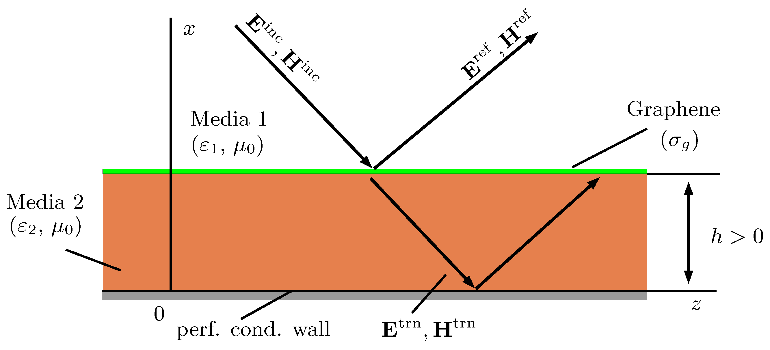
2. Statement of the Problem

Below we consider the scattering of optical waves by a slab covered with a graphene monolayer. It is assumed that the wavelength of an incident light as well as the thickness of the slab (>100 nm) is by several orders larger than the thickness of a monolayer of graphene (≈0.33 nm). Note that in the visible and near infrared region the wavelength of an optical wave is by 3–4 orders larger than the thickness of graphene monolayer. Thus, we can well represent the graphene coating as an infinitely thin sheet with a nonzero surface conductivity. From the point of view of classical electrodynamics, its effect on the propagation of optical waves is given by boundary conditions at the interfaces of graphene sheet with the neighbouring media [32]. Besides, the slab is assumed to be regular and infinite in two directions and the incident wave is assumed to be TE-polarized. As it is known, in this case components of the electromagnetic field depend only on two spatial variables and the original three-dimensional problem actually degenerates into a two-dimensional one. So, we prefer to give the statement of the problem directly in ${\mathbb{R}}^2$.

Let us define sets

$$\begin{array}{cc}\hfill {\Omega }_1:=\{(x,z):x>h,z\in \mathbb{R}\},& {\Omega }_2:=\{(x,z):0<x<h,z\in \mathbb{R}\},\hfill \\ \hfill {\Gamma }_0:=\{(x,z):x=0,z\in \mathbb{R}\},& {\Gamma }_h:=\{(x,z):x=h,z\in \mathbb{R}\},\hfill \end{array}$$

where h is a positive constant.

Consider a two-dimensional infinite slab ${\Omega }_2$ of thickness h coated with a sheet of graphene at interface ${\Gamma }_h$ and having a perfectly conducting wall at interface ${\Gamma }_0$. The former interface is illuminated by a monochromatic TE-polarized light ${\mathbf{E}}^{\mathrm{inc}}exp(-i\omega t)$, ${\mathbf{H}}^{\mathrm{inc}}exp(-i\omega t)$ coming from half-plane ${\Omega }_1$. Complex amplitudes ${\mathbf{E}}^{\mathrm{inc}}$, ${\mathbf{H}}^{\mathrm{inc}}$ have the form

$${\mathbf{E}}^{\mathrm{inc}}=\left(0,{\mathrm{E}}_y^{\mathrm{inc}}(x,z),0\right),{\mathbf{H}}^{\mathrm{inc}}=\left({\mathrm{H}}_x^{\mathrm{inc}}(x,z),0,{\mathrm{H}}_z^{\mathrm{inc}}(x,z)\right).$$

Both regions ${\Omega }_1$ and ${\Omega }_2$ are filled with isotropic homogeneous media characterized by (relative) dielectric constants ${\epsilon }_1$ and ${\epsilon }_2$, respectively, and magnetic constant $\mu ={\mu }_0$, where ${\mu }_0$ is the permeability of free space.

Passing through interface ${\Gamma }_h$, the incident light is partially reflected and partially transmitted. Let $\left({\mathbf{E}}^{\mathrm{ref}},{\mathbf{H}}^{\mathrm{ref}}\right)exp(-i\omega t)$, $\left({\mathbf{E}}^{\mathrm{trn}},{\mathbf{H}}^{\mathrm{trn}}\right)exp(-i\omega t)$ denote reflected and transmitted parts of the incident light, respectively. Then the total electromagnetic field has the form $\left({\mathbf{E}}^{\mathrm{tot}},{\mathbf{H}}^{\mathrm{tot}}\right)exp(-i\omega t)$, where

$${\mathbf{E}}^{\mathrm{tot}}=\left\{\begin{array}{cc}{\mathbf{E}}^{\mathrm{ref}}+{\mathbf{E}}^{\mathrm{inc}},\hfill & (x,z)\in {\Omega }_1,\hfill \\ {\mathbf{E}}^{\mathrm{trn}},\hfill & (x,z)\in {\Omega }_2,\hfill \end{array}\right.{\mathbf{H}}^{\mathrm{tot}}=\left\{\begin{array}{cc}{\mathbf{H}}^{\mathrm{ref}}+{\mathbf{H}}^{\mathrm{inc}},\hfill & (x,z)\in {\Omega }_1,\hfill \\ {\mathbf{H}}^{\mathrm{trn}},\hfill & (x,z)\in {\Omega }_2.\hfill \end{array}\right.$$

Assuming that reflected and transmitted fields have the same polarization as the incident light, one can write

$$\begin{array}{cc}\hfill {\mathbf{E}}^{\mathrm{ref}}& =\left(0,{\mathrm{E}}_y^{\mathrm{ref}}(x,z),0\right),{\mathbf{H}}^{\mathrm{ref}}=\left({\mathrm{H}}_x^{\mathrm{ref}}(x,z),0,{\mathrm{H}}_z^{\mathrm{ref}}(x,z)\right),\hfill \\ \hfill {\mathbf{E}}^{\mathrm{trn}}& =\left(0,{\mathrm{E}}_y^{\mathrm{trn}}(x,z),0\right),{\mathbf{H}}^{\mathrm{trn}}=\left({\mathrm{H}}_x^{\mathrm{trn}}(x,z),0,{\mathrm{H}}_z^{\mathrm{trn}}(x,z)\right).\hfill \end{array}$$

A schematic of the above physical model is presented in Figure 1.

Complex amplitudes ${\mathbf{E}}^{\mathrm{tot}}$, ${\mathbf{H}}^{\mathrm{tot}}$ must satisfy Maxwell’s equations

$$\left\{\begin{array}{cc}\mathrm{rot}{\mathbf{H}}^{\mathrm{tot}}\hfill & =-i\omega {ϵ}_0{\epsilon }_r{\mathbf{E}}^{\mathrm{tot}},\hfill \\ \mathrm{rot}{\mathbf{E}}^{\mathrm{tot}}\hfill & =i\omega {\mu }_0{\mathbf{H}}^{\mathrm{tot}},\hfill \end{array}\right.$$

where ${ϵ}_0$ is the dielectric permittivity of free space and

$${\epsilon }_r=\left\{\begin{array}{cc}{\epsilon }_1,\hfill & (x,z)\in {\Omega }_1,\hfill \\ {\epsilon }_2,\hfill & (x,z)\in {\Omega }_2.\hfill \end{array}\right.$$

Tangential component ${\mathbf{E}}_{\tau }^{\mathrm{tot}}$ of the electric field must vanish at interface ${\Gamma }_0$ implying the following boundary conditions

$${\left.{\mathbf{E}}_{\tau }^{\mathrm{tot}}\right|}_{x=0+0}=0.$$

At interface ${\Gamma }_h$ one has coupling condition

$${\left.[\mathbf{n},{\mathbf{H}}^{\mathrm{tot}}]\right|}_{x=h+0}-{\left.[\mathbf{n},{\mathbf{H}}^{\mathrm{tot}}]\right|}_{x=h-0}={\left.{\sigma }_g{\mathbf{E}}_{\tau }^{\mathrm{tot}}\right|}_{x=h-0},$$

where $\mathbf{n}=(1,0,0)$ is a unit normal vector directed along the x-th direction, $[·,·]$ is the operation of vector product and ${\sigma }_g$ is the conductivity of graphene. Finally reflected ${\mathbf{E}}^{\mathrm{ref}}$, ${\mathbf{H}}^{\mathrm{ref}}$ and incident ${\mathbf{E}}^{\mathrm{inc}}$, ${\mathbf{H}}^{\mathrm{inc}}$ fields must satisfy Sommerfeld radiation condition.

Conductivity ${\sigma }_g$ of graphene nonlinearly depends on the value of the tangential component of the electric field. In accordance with [12] we assume that

$${\sigma }_g={\sigma }^{\left(1\right)}+{\left.{\sigma }^{\left(3\right)}{\left|{\mathbf{E}}_{\tau }^{\mathrm{tot}}\right|}^2\right|}_{x=h},$$

where ${\sigma }^{\left(1\right)}$, ${\sigma }^{\left(3\right)}$ are some complex quantities depending on the temperature and the chemical potential of graphene as well as the frequency of an incident electromagnetic wave. Explicit formulas for ${\sigma }^{\left(1\right)}$, ${\sigma }^{\left(3\right)}$ will be given in Section 4.

Let us introduce notation $k_0^2={\omega }^2{ϵ}_0{\mu }_0$, $k_1^2={\epsilon }_1$, $k_2^2={\epsilon }_2$, $u_1(x,z):={\mathrm{E}}_y^{\mathrm{ref}}(x,z)$, $u_2(x,z):={\mathrm{E}}_y^{\mathrm{trn}}(x,z)$, $u_{\mathrm{inc}}:={\mathrm{E}}_y^{\mathrm{inc}}(x,z)$.

The above electromagnetic problem is equivalent to a transmission problem which is to find a pair of functions $u_1\equiv u_1(x,z)\in C^2\left({\Omega }_1\right)\cap C\left({\overline{\Omega }}_1\right)$, $u_2\equiv u_2(x,z)\in C^2\left({\Omega }_2\right)\cap C\left({\overline{\Omega }}_2\right)$ satisfying Helmholtz equations

$$\begin{array}{cc}\hfill \Delta u_1+k_1^2{u}_1 = 0,& (x,z)\in {\Omega }_1,\hfill \end{array}$$

(1)

$$\begin{array}{cc}\hfill \Delta u_2+k_2^2{u}_2 = 0,& (x,z)\in {\Omega }_2,\hfill \end{array}$$

(2)

vanishing condition at interface ${\Gamma }_0$, i.e.,

$$u_2{|}_{x=0}=0,$$

(3)

continuity condition at interface ${\Gamma }_h$, i.e.,

$${\left.u_1\right|}_{x=h+0}-{\left.u_2\right|}_{x=h-0}=-{\left.u_{\mathrm{inc}}\right|}_{x=h+0},$$

(4)

graphene-caused coupling condition

$${\left.{\displaystyle \frac{\partial u_1}{\partial x}}\right|}_{x=h+0}-{\left.{\displaystyle \frac{\partial u_2}{\partial x}}\right|}_{x=h-0}-{\left.\gamma {\sigma }_g{u}_2\right|}_{x=h-0}=-{\left.{\displaystyle \frac{\partial u_{\mathrm{inc}}}{\partial x}}\right|}_{x=h+0},$$

(5)

where $\gamma ={\left(ic{ϵ}_0\right)}^{-1}$, and Sommerfeld radiation condition

$$\underset{r\to \infty }{lim}\sqrt{r}{u}_1=\mathrm{const},\underset{r\to \infty }{lim}\sqrt{r}\left({\displaystyle \frac{\partial u_1}{\partial r}}+i{k}_1{u}_1\right)=0,r=\sqrt{x^2+z^2}.$$

(6)

Here spatial coordinates are normalized to the inverse wave number $k_0$.

As $u_{\mathrm{inc}}$ we use function

$$u_{\mathrm{inc}}(x,z)={\displaystyle \frac{i{f}_0}{4}}{H}_0^{\left(1\right)}\left(k_1\sqrt{{(x-x_0)}^2+{(z-z_0)}^2}\right)$$

(7)

satisfying Helmholtz equation

$$\Delta u+k_1^{2}u=f_0\delta (x-x_0)\delta (z-z_0).$$

Here $H_0^{\left(1\right)}$ is a Hankel function of the first kind and $f_0>0$, $x_0$, $z_0$ are real parameters. From a physical point of view, Formula (7) is a 2D analogue of an electromagnetic field produced by a classical (3D) point source. Parameters $x_0$, $z_0$ determine the location of the source; as it is situated in region ${\Omega }_1$, then $x_0>h$. Parameter $f_0$ has dimension of V/m and determines the power of the source.

Function $u_{\mathrm{uic}}(x,z)$ for $k_1=1$, $x_0=6$, $z_0=0$ and $f_0=1$ V/m is plotted in Figure 2 (the same values for $k_1$, $x_0$, $z_0$ are used for calculations in Section 4).

3. Methods

To study transmission problems, they are often reduced to a single boundary integral equation [33,34]. This is what we do in Section 3.1. The obtained boundary integral equation has two significant features. Firstly, it involves a hypersingular integral operator which is notoriously difficult to calculate numerically. Secondly, it is nonlinear with respect to a sought-for function. To find an approximate solution to this equation, we develop a novel method described in Section 3.2 and Section 3.3.

3.1. Reduction to a Single Boundary Integral Equation

Solution $u_1\equiv u_1(x,z)$ to Equation (1) can be presented in the form

$$u_1(x,z)=\underset{-\infty }{\overset{+\infty }{\int }}{v}_1\left(\eta \right){\left.\left[{\displaystyle \frac{\partial }{\partial \xi }}{G}_1(x,z,\xi ,\eta )\right]\right|}_{\xi =h}d\eta ,$$

where $v_1\left(\eta \right)$ is the trace of $u_1$ at interface ${\Gamma }_h$ and $G_1$ is a Green’s function of the Dirichlet problem for 2D Helmholtz equation in region ${\Omega }_1$. Analogically, solution $u_2$ to Equation (2) can be written in the form

$$u_2(x,z)=\underset{-\infty }{\overset{+\infty }{\int }}{v}_0\left(\eta \right){\left.\left[{\displaystyle \frac{\partial }{\partial \xi }}{G}_2(x,z,\xi ,\eta )\right]\right|}_{\xi =0}d\eta -\underset{-\infty }{\overset{+\infty }{\int }}{v}_2\left(\eta \right){\left.\left[{\displaystyle \frac{\partial }{\partial \xi }}{G}_2(x,z,\xi ,\eta )\right]\right|}_{\xi =h}d\eta ,$$

where $v_0\left(\eta \right)$ and $v_2\left(\eta \right)$ are traces of $u_2$ at interfaces ${\Gamma }_0$ and ${\Gamma }_h$, respectively, and $G_2$ is a Green’s function of the Dirichlet problem for 2D Helmholtz equation in region ${\Omega }_2$. As it is known, for a half-plane and an infinite strip there are explicit expressions of the specified Green’s functions. We present them in Appendix A and Appendix B.

From condition (3) it follows that in the above formula $v_0$ equals zero.

Let us introduce notation

$$\begin{array}{cc}\hfill f\left(z\right)& =u_{\mathrm{inc}}{(x,z)|}_{x=h+0}={\displaystyle \frac{i{f}_0}{4}}{H}_0^{\left(1\right)}\left(k_1\sqrt{b^2+{(z-z_0)}^2}\right),\hfill \\ \hfill f^{\prime }\left(z\right)& ={\left.{\displaystyle \frac{\partial u_{\mathrm{inc}}(x,z)}{\partial x}}\right|}_{x=h+0}=-{\displaystyle \frac{i{f}_0{k}_{1}b}{4}}{\displaystyle \frac{H_1^{\left(1\right)}\left(k_1\sqrt{b^2+{(z-z_0)}^2}\right)}{\sqrt{b^2+{(z-z_0)}^2}}},\hfill \end{array}$$

where $b=h-x_0$. Using coupling condition (4), one gets

$$v_1\left(\eta \right)=v_2\left(\eta \right)-f\left(\eta \right)=v\left(\eta \right)-f\left(\eta \right).$$

Hence it follows that

$$u_1(x,z)=\underset{-\infty }{\overset{+\infty }{\int }}v\left(\eta \right){\left.\left[{\displaystyle \frac{\partial }{\partial \xi }}{G}_1(x,z,\xi ,\eta )\right]\right|}_{\xi =h}d\eta -\underset{-\infty }{\overset{+\infty }{\int }}f\left(\eta \right){\left.\left[{\displaystyle \frac{\partial }{\partial \xi }}{G}_1(x,z,\xi ,\eta )\right]\right|}_{\xi =h}d\eta$$

(8)

and

$$u_2(x,z)=-\underset{-\infty }{\overset{+\infty }{\int }}v\left(\eta \right){\left.\left[{\displaystyle \frac{\partial }{\partial \xi }}{G}_2(x,z,\xi ,\eta )\right]\right|}_{\xi =h}d\eta .$$

(9)

Substituting the above expressions for $u_1$ and $u_2$ into condition (5), one obtains

$$\left({\mathcal{N}}_{2}v\right)\left(z\right)+\left({\mathcal{N}}_{1}v\right)\left(z\right)-\gamma {\sigma }_{g}v\left(z\right)=F\left(z\right),$$

(10)

where $F\left(z\right)=\left({\mathcal{N}}_{1}f\right)\left(z\right)-f^{\prime }\left(z\right)$ and

$$\left({\mathcal{N}}_j\phi \right)\left(z\right)={\displaystyle \frac{\partial }{\partial x}}{\left.\left[\underset{-\infty }{\overset{+\infty }{\int }}\phi \left(\eta \right){\left.{\displaystyle \frac{\partial G_j(x,z,\xi ,\eta )}{\partial \xi }}\right|}_{\xi =h}d\eta \right]\right|}_{x=h}.$$

(11)

Note that integral operators ${\mathcal{N}}_1$, ${\mathcal{N}}_2$ are hypersingular. Besides, ${\sigma }_g={\sigma }^{\left(1\right)}+{\sigma }^{\left(3\right)}{\left|v\right|}^2$, i.e., Equation (10) is nonlinear with respect to the sought-for function.

So, the transmission problem (1)–(6) is reduced to nonlinear hypersingular boundary integral Equation (10). As it is known, a hypersingular integral operator is difficult to calculate numerically. At the same time, there is an effective way to calculate them analytically. For this, one should replace the sought-for function by a Chebyshev series and use an explicit formula for the action of a hypersingular integral operator on a Chebyshev polynomial of the second kind [35,36,37]. However, this technique cannot be directly applied to operators ${\mathcal{N}}_j$. So, in the next section we reduce Equation (10) and operators ${\mathcal{N}}_j$ to the form suitable for using the specified method.

3.2. Analytical Calculation of Hypersingular Integral Operators

Everywhere below index j takes values $1,2$.

Being fundamental solutions to a 2D Helmholtz equation functions $G_j$ have a logarithmic singularity. At the same time, being solutions to the Dirichlet problem functions $G_j$ vanish at interface ${\Gamma }_h$. Taking that into account, one can present $G_j$ as follows

$$\begin{array}{c}{G}_j(x,z,\xi ,\eta )={\displaystyle \frac{1}{2\pi }}ln\sqrt{{\left(x-\xi \right)}^2+{(z-\eta )}^2}-\hfill \\ \hspace{1em}\hspace{1em}\hspace{1em}\hspace{1em}\hspace{1em}\hspace{1em}\hspace{1em} -{\displaystyle \frac{1}{2\pi }}ln\sqrt{{\left(x-2h+\xi \right)}^2+{(z-\eta )}^2}+{\mathsf{\Phi }}_j(x,z,\xi ,\eta )-{\mathsf{\Phi }}_j(x,z,h,\eta ),\hfill \end{array}$$

where ${\mathsf{\Phi }}_j$ are continuous functions. Differentiating $G_j$ twice with respect to $\xi$ and x and computing the result at $\xi =h$, one gets

$${\left.{\displaystyle \frac{{\partial }^2{G}_j(x,z,\xi ,\eta )}{\partial x\partial \xi }}\right|}_{\xi =h}={\displaystyle \frac{1}{\pi }}{\displaystyle \frac{\partial }{\partial z}}\left[{\displaystyle \frac{(z-\eta )}{{(x-h)}^2+{(z-\eta )}^2}}\right]+{\left.{\displaystyle \frac{{\partial }^2{\mathsf{\Phi }}_j(x,z,\xi ,\eta )}{\partial x\partial \xi }}\right|}_{\xi =h}.$$

Substituting these expressions into ${\mathcal{N}}_j$, we obtain

$$\left({\mathcal{N}}_j\phi \right)\left(z\right)={\displaystyle \frac{1}{\pi }}{\displaystyle \frac{\partial }{\partial z}}\underset{-\infty }{\overset{+\infty }{\int }}{\displaystyle \frac{1}{z-\eta }}\phi \left(\eta \right)d\eta +\underset{-\infty }{\overset{+\infty }{\int }}{K}_j(z,\eta )\phi \left(\eta \right)d\eta ,$$

(12)

where

$$K_j(z,\eta )={\left.{\displaystyle \frac{{\partial }^2{\mathsf{\Phi }}_j(x,z,\xi ,\eta )}{\partial x\partial \xi }}\right|}_{{\Gamma }_h}.$$

Detailed derivation of (12) is given in Appendix A and Appendix B.

Though we do not provide explicit formulas for $K_j$ in this part of the paper, it is worth noting that both $K_1$ and $K_2$ have a logarithmic singularity for $z=\eta$ and are continuous as $\eta$ tends to $\pm \infty$.

Introduce new variables $\zeta$ and p related to z, $\eta$ by formulas

$$z=ln{\displaystyle \frac{1+\zeta }{1-\zeta }},\eta =ln{\displaystyle \frac{1+p}{1-p}}.$$

(13)

Equation (10) in variables $\zeta$, p takes the form

$$2\left(\mathcal{S}\tilde{v}\right)\left(\zeta \right)+2\sum _j\left({\mathcal{K}}_j\tilde{v}\right)\left(\zeta \right)-\gamma {\sigma }_g\tilde{v}\left(\zeta \right)=\tilde{F}\left(\zeta \right),$$

where

$$\tilde{v}\left(\zeta \right)=v\left(ln{\displaystyle \frac{1+\zeta }{1-\zeta }}\right),\tilde{F}\left(\zeta \right)=F\left(ln{\displaystyle \frac{1+\zeta }{1-\zeta }}\right),$$

operators $\mathcal{S}$, ${\mathcal{K}}_j$ are defined by formulas

$$\begin{array}{cc}\hfill \left(\mathcal{S}\tilde{v}\right)\left(\zeta \right)& ={\displaystyle \frac{1-{\zeta }^2}{2\pi }}{\displaystyle \frac{d}{d\zeta }}\underset{-1}{\overset{1}{\int }}{\mathrm{arctanh}}^{-1}\left({\displaystyle \frac{\zeta -p}{1-p\zeta }}\right)\tilde{v}\left(p\right){\displaystyle \frac{dp}{1-p^2}},\hfill \\ \hfill \left({\mathcal{K}}_j\tilde{v}\right)\left(\zeta \right)& =\underset{-1}{\overset{1}{\int }}{\tilde{K}}_j\left(\zeta ,p\right)\tilde{v}\left(p\right){\displaystyle \frac{dp}{1-p^2}}\hfill \end{array}$$

and kernels ${\tilde{K}}_j$ have form

$${\tilde{K}}_j\left(\zeta ,p\right)=K_j\left(ln{\displaystyle \frac{1+\zeta }{1-\zeta }},ln{\displaystyle \frac{1+p}{1-p}}\right).$$

In deriving the above equation we used relation

$$ln{\displaystyle \frac{1+t}{1-t}}=2\mathrm{arctanh}t,\mathrm{arctanh}{t}_1-\mathrm{arctanh}{t}_2=\mathrm{arctanh}\left({\displaystyle \frac{t_1-t_2}{1-t_1{t}_2}}\right).$$

In addition, operator $\mathcal{S}$ can be presented as a sum $\mathcal{S}=\mathcal{H}+{\mathcal{K}}_3$, where

$$\begin{array}{cc}\hfill \left(\mathcal{H}\tilde{v}\right)\left(\zeta \right)& ={\displaystyle \frac{1}{2\pi }}(1-{\zeta }^2){\displaystyle \frac{d}{d\zeta }}\underset{-1}{\overset{1}{\int }}{\displaystyle \frac{1}{\zeta -p}}\tilde{v}\left(p\right)dp,\hfill \\ \hfill \left({\mathcal{K}}_3\tilde{v}\right)\left(\zeta \right)& =\underset{-1}{\overset{1}{\int }}{\tilde{K}}_3(\zeta ,p)\tilde{v}\left(p\right){\displaystyle \frac{dp}{1-p^2}}\hfill \end{array}$$

and

$${\tilde{K}}_3(\zeta ,p)=-{\displaystyle \frac{1}{2\pi }}\left(1-{\displaystyle \frac{{(1-p\zeta )}^2}{{(\zeta -p)}^2}}+{\mathrm{arctanh}}^{-2}{\displaystyle \frac{\zeta -p}{1-p\zeta }}\right).$$

(14)

By virtue of the Maclaurin series expansion one can check that the kernel of integral operator ${\mathcal{K}}_3$ is continuous.

Thus, we come to integral equation

$$2\left(\mathcal{H}\tilde{v}\right)\left(\zeta \right)+2\sum _{i=1}^3\left({\mathcal{K}}_i\tilde{v}\right)\left(\zeta \right)-\gamma {\sigma }_g\tilde{v}\left(\zeta \right)=\tilde{F}\left(\zeta \right).$$

(15)

Clearly, operator $\mathcal{H}$ is hypersingular. The important thing is that it has such a form that one can straightforwardly compute $\mathcal{H}$ using Chebyshev polynomials.

Indeed, let us present the sought-for function v in the form

$$\tilde{v}\left(p\right)=\sqrt{1-p^2}·\sum _{n=0}^{+\infty }{c}_n{U}_n\left(p\right),$$

(16)

where $U_n$ are Chebyshev polynomials of the second kind and $c_n$ are some coefficients. Substituting this series into $\mathcal{H}$ and using relations [35]

$$\underset{-1}{\overset{1}{\int }}{\displaystyle \frac{1}{t-s}}{U}_{n-1}\left(t\right)\sqrt{1-t^2}dt=-\pi T_n\left(s\right),U_n\left(s\right)={\displaystyle \frac{1}{n+1}}{T}_{n+1}^{\prime }\left(s\right),$$

one finds

$$\left(\mathcal{H}\tilde{v}\right)\left(\zeta \right)={\displaystyle \frac{1}{2}}\sum _{n=0}^{+\infty }{c}_n(n+1)(1-{\zeta }^2)U_n\left(\zeta \right).$$

Let index i take values $1,2,3$. Substituting series (16) into operators ${\mathcal{K}}_i$, they take the form

$$\left({\mathcal{K}}_i\tilde{v}\right)\left(\zeta \right)=\sum _{n=0}^{+\infty }{c}_n\underset{-1}{\overset{1}{\int }}{\tilde{K}}_i(\zeta ,p)U_n\left(p\right){\displaystyle \frac{dp}{\sqrt{1-p^2}}}.$$

In the above integrals, it makes sense to pass to integration variable $\theta =arccosp$. Using relation

$$U_n\left(p\right)={\displaystyle \frac{1}{\sqrt{1-p^2}}}·sin\left((n+1)arccosp\right),$$

we come to formulas

$$\left({\mathcal{K}}_i\tilde{v}\right)\left(\zeta \right)=\sum _{n=0}^{+\infty }{c}_n\underset{0}{\overset{\pi }{\int }}{\tilde{K}}_i\left(\zeta ,cos\theta \right){\displaystyle \frac{sin(n+1)\theta }{sin\theta }}d\theta =\sum _{n=0}^{+\infty }{c}_n{K}_i^{\left(n\right)}\left(\zeta \right).$$

We stress that integrals $K_i^{\left(n\right)}$ are convergent. Indeed, as mentioned above, kernels ${\tilde{K}}_1$ and ${\tilde{K}}_2$ have an integrable (logarithmic) singularity if the arguments coincide and are continuous as $\theta$ approaches the edges 0, $\pi$. Kernel ${\tilde{K}}_3(\zeta ,cos\theta )$ is continuous on the entire region $(\zeta ,\theta )\in [-1,1]\times [0,\pi ]$. Thus, to show the convergence of integrals $K_i^{\left(n\right)}$, it remains to notice that

$$\underset{\theta \to 0}{lim}{\displaystyle \frac{sin(n+1)\theta }{sin\theta }}=n+1,\underset{\theta \to \pi }{lim}{\displaystyle \frac{sin(n+1)\theta }{sin\theta }}={(-1)}^n(n+1).$$

Uniting the obtained results, one arrives at the equation

$$\sum _{n=0}^{+\infty }{c}_n\left({\mathrm{{\rm Y}}}_n\left(\zeta \right)-\gamma {\sigma }_{g}sin\left.\left(\right(n+1)arccos\zeta \right)\right)=\tilde{F}\left(\zeta \right),$$

(17)

where $\zeta \in [-1,1]$ and

$${\mathrm{{\rm Y}}}_n\left(\zeta \right)=(n+1)\sqrt{1-{\zeta }^2}sin\left.\left(\right(n+1)arccos\zeta \right)+2\sum _{i=1}^3{K}_i^{\left(n\right)}\left(\zeta \right).$$

The obtained equation has two crucial peculiarities. Firstly, it is defined on a finite segment $\zeta \in [-1,1]$, whereas the original boundary integral Equation (10) is defined on the whole $\mathbb{R}$. Secondly, and most importantly, all integrals $K_i^{\left(n\right)}$ in the left-hand side of (17) have either a continuous kernel or a kernel with logarithmic singularity and thus are easily calculated numerically. It should be noted that there is still a hypersingular integral operator in the right-hand side of (17), see the definition of function $\tilde{F}$. However, since it is acting on known function f, one can try to calculate it straightforwardly as it is done in Appendix C.

Remind that Equation (17) is nonlinear with respect to the sought-for function because

$${\sigma }_g={\sigma }^{\left(1\right)}+{\sigma }^{\left(3\right)}{\left|\tilde{v}\right|}^2\left(\zeta \right).$$

(18)

To find an approximate solution of this equation, we use an approach based on the collocation method combined with an iterative one. It is described in detail in Section 3.3.

3.3. Collocation Method & Iterative Scheme

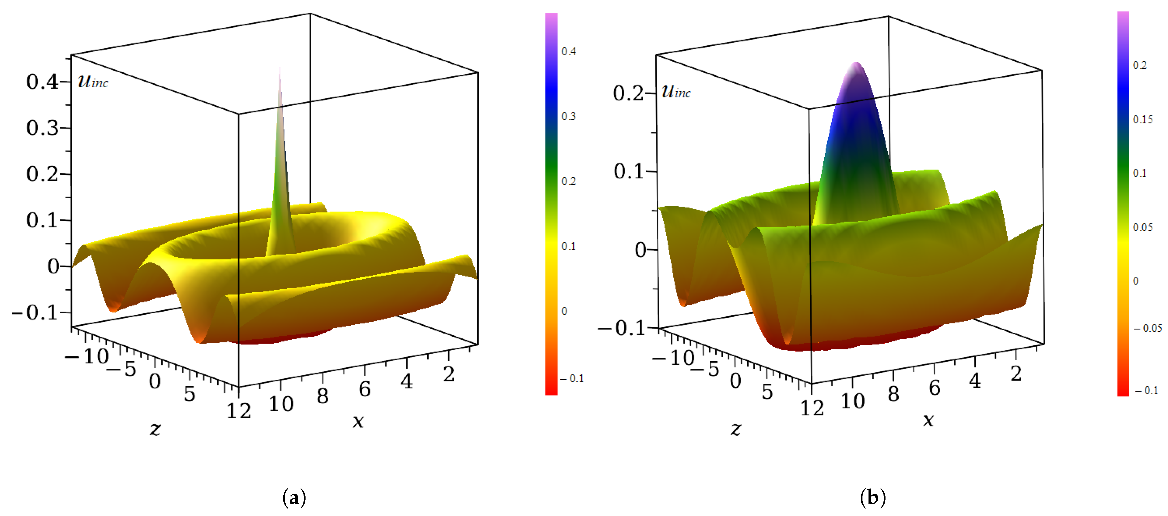
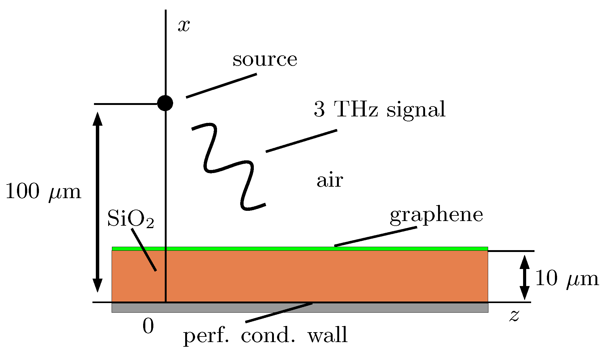
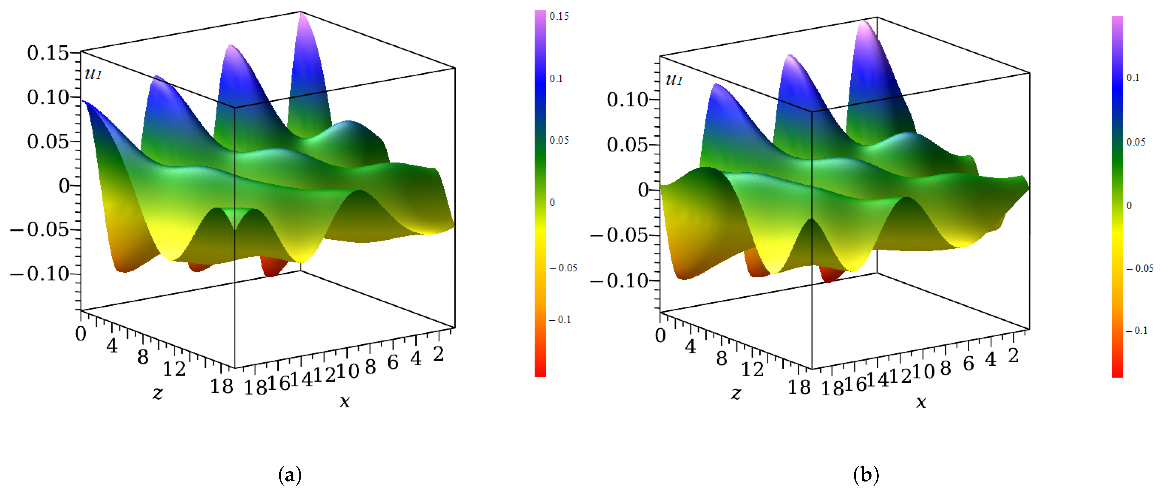
At fist, assume that ${\sigma }^{\left(3\right)}=0$. In this case Equation (17) is linear and one can use the classical collocation method to find its approximate solution.

Let us introduce the following grid

$$-1<{\zeta }_0<{\zeta }_1<\dots <{\zeta }_N<1$$

with nodes being the roots of a Chebyshev polynomial $U_{N+1}\left(\zeta \right)$. We look for an approximate solution of Equation (17) in the form

$${\tilde{v}}_N\left(\zeta \right)=\sqrt{1-{\zeta }^2}·\sum _{n=0}^N{c}_n{U}_n\left(\zeta \right)$$

(19)

with coefficients determined from the system of $N+1$ equations

$$\sum _{n=0}^N{c}_n\left[{\mathrm{{\rm Y}}}_n\left({\zeta }_k\right)-\gamma {\sigma }^{\left(1\right)}sin\left.((n+1)arccos{\zeta }_k\right)\right]=\tilde{F}\left({\zeta }_k\right),$$

(20)

that can be solved using the Gauss-Jordan elimination or some iterative method.

Let ${\sigma }^{\left(3\right)}$ now be different from zero. Clearly, in Formula (18) term ${\sigma }^{\left(3\right)}{\left|\tilde{v}\right|}^2$ is a small correction to ${\sigma }^{\left(1\right)}$. It implies that, as before, we can look for an approximate solution of Equation (17) in the form

$${\tilde{v}}_{N,M}\left(\zeta \right)=\sqrt{1-{\zeta }^2}·\sum _{n=0}^N{c}_n^{\left(M\right)}{U}_n\left(\zeta \right)$$

(21)

with coefficients determined via the following iterative scheme

$$\sum _{n=0}^N{c}_n^{(M+1)}\left[{\mathrm{{\rm Y}}}_n\left({\zeta }_k\right)-\gamma sin\left.((n+1)arccos{\zeta }_k\right)·{\sigma }_{N,M}\left({\zeta }_k\right)\right]=\tilde{F}\left({\zeta }_k\right),$$

(22)

where $M=0,1,\dots ,$ and

$${\sigma }_{N,M}\left(\zeta \right)={\sigma }^{\left(1\right)}+{\sigma }^{\left(3\right)}{\left|{\tilde{v}}_{N,M}\right|}^2\left(\zeta \right).$$

As an initial approximation ${\tilde{v}}_{N,0}$ it makes sense to use the linear solution ${\tilde{v}}_N$.

Clearly, in order to obtain a good approximate solution of Equation (17), one should increase the number of terms in sum (21) as well as the number of iterations in the scheme (22) until the distance between the current solution

$${\tilde{v}}^{**}\left(\zeta \right)=\sqrt{1-{\zeta }^2}\sum _{n=0}^{N^{**}}{c}_n^{**}{U}_n\left(\zeta \right)$$

and the previous one

$${\tilde{v}}^{*}\left(\zeta \right)=\sqrt{1-{\zeta }^2}\sum _{n=0}^{N^{*}}{c}_n^{*}{U}_n\left(\zeta \right)$$

becomes smaller than a given positive number $\delta$. By distance, we mean the uniform norm $\parallel {\tilde{v}}^{**}\left(\zeta \right)-{\tilde{v}}^{*}\left(\zeta \right)\parallel$ which can be evaluated as follows

$$\begin{array}{c}\parallel {\tilde{v}}^{**}\left(\zeta \right)-{\tilde{v}}^{*}\left(\zeta \right)\parallel =\underset{\zeta \in [-1,1]}{max}\left.|{\tilde{v}}^{**}\left(\zeta \right)-{\tilde{v}}^{*}\left(\zeta \right)\right|⩽\hfill \\ \hfill \hspace{1em}\hspace{1em}\hspace{1em}\hspace{1em}\hspace{1em}\hspace{1em}\hspace{1em}\hspace{1em}\hspace{1em}⩽{\displaystyle \sum _{n=0}^{N^{**}}}{\theta }_n\underset{\zeta \in [-1,1]}{max}|\sqrt{1-{\zeta }^2}·U_n\left(\zeta \right)|⩽{\displaystyle \sum _{n=0}^{N^{**}}}{\theta }_n=D\left({\tilde{v}}^{**},{\tilde{v}}^{*}\right),\end{array}$$

(23)

where quantities ${\theta }_n$ are defined by formula

$${\theta }_n=\left\{\begin{array}{cc}|c_n^{**}-c_n^{*}|,\hfill & 0⩽n⩽N^{*},\hfill \\ |c_n^{**}|,\hfill & N^{*}<n⩽N^{**}.\hfill \end{array}\right.$$

Remind that by definition solution $\tilde{v}$ of Equation (17) describes the electric field at interface ${\Gamma }_h$ from inside the slab and the electric field at interface ${\Gamma }_h$ from outside the slab is determined as $\tilde{v}-f$. To calculate the electric field at a given point beyond ${\Gamma }_h$, one should use Formulas (8) and (9). Note that the integrands involved in (8), (9) have no singularities at points beyond interface ${\Gamma }_h$ and thus can be easily calculated numerically.

Figure 3 shows a diagram describing the main milestones of the above method.

4. Results

The linear part of the conductivity of graphene consists of intra- and interband contributions, i.e., ${\sigma }^{\left(1\right)}={\sigma }_{\mathrm{intra}}+{\sigma }_{\mathrm{inter}}$. Assuming that graphene is highly doped $|{\mu }_c|\gg k_{b}T$, ${\mu }_c$ is a chemical potential, and excitation is below interband absorption threshold $\hslash \omega <2|{\mu }_c|$, both these terms are given by the semi-classical formalism

$$\begin{array}{cc}\hfill {\sigma }_{\mathrm{intra}}(\Omega )& ={\displaystyle \frac{i{e}^2}{\pi \hslash }}{\displaystyle \frac{1}{\Omega +i{\nu }_{\mathrm{intra}}}},\hfill \\ \hfill {\sigma }_{\mathrm{inter}}(\Omega )& ={\displaystyle \frac{i{e}^2}{4\pi \hslash }}ln{\displaystyle \frac{2-|\Omega |-i{\nu }_{\mathrm{inter}}}{2+|\Omega |+i{\nu }_{\mathrm{inter}}}},\hfill \end{array}$$

where $\Omega =\hslash \omega /{\mu }_c$, ${\nu }_{\mathrm{intra}}=\hslash /\left(\right|{\mu }_c\left|{\tau }_{\mathrm{intra}}\right)$, ${\nu }_{\mathrm{inter}}=\hslash /\left(\right|{\mu }_c\left|{\tau }_{\mathrm{inter}}\right)$ [38]. The latter two quantities take into account losses due to electron scatterings at finite temperatures. Below we use ${\tau }_{\mathrm{intra}}=100$ fs, ${\tau }_{\mathrm{inter}}=1$ ps [39,40] and ${\mu }_c=0.1$ eV (except for Figure 7 where different values for ${\mu }_c$ are used).

Nonlinear conductivity coefficient ${\sigma }^{\left(3\right)}$ for graphene is given by

$${\sigma }^{\left(3\right)}(\Omega )=-i{\displaystyle \frac{3}{32}}{\displaystyle \frac{e^2}{\pi \hslash }}{\displaystyle \frac{{\left(e{V}_F\right)}^2{\hslash }^2}{{\mu }_c^4{\Omega }^3}},$$

where $V_F$ is the Fermi velocity [12].

In calculations we use the following parameters for the waveguiding structure: $k_1^2={\epsilon }_1=1$ (air), $k_2^2={\epsilon }_2=4$ (close to the dielectric constant ($3.9$) of ${\mathrm{SiO}}_2$), $h=0.6$. Let the light source be placed at the point with coordinates $x_0=6$, $z_0=0$ and emit monochromatic light at frequency $\omega /2\pi =3$ THz. For the nonlinearity of graphene to become noticeable, the amplitude of the incident light should be sufficiently large. We use $f_0=50$ MV/m.

Note that dimensionless thickness h of slab ${\Omega }_2$ should correlate with its physical size. Indeed, it should be calculated by formula $h=k_0\tilde{h}$, where $\tilde{h}$ is the real thickness of the slab. Assume that $\tilde{h}=10$ $\mathsf{\mu }$m [27]. For $\omega /2\pi =3$ THz we have $k_0\approx 6·{10}^4{\mathrm{m}}^{-1}$. Hence one finds $h\approx 0.6$. Similarly, dimensionless $x_0=6$ corresponds to ${\tilde{x}}_0=k_0^{-1}{x}_0\approx 100$ $\mathsf{\mu }$m.

The sketch of the described above waveguide is shown in Figure 4.

Introduce sequence $a_k=kd$, $k=1,2,\dots$, with a common difference $d=96$ (the value of d is chosen to be a multiple of the number of processors that we use for parallel computing). Let ${\tilde{v}}_{\left(k\right)}\left(\zeta \right)$ and ${\tilde{v}}_{(k,m)}\left(\zeta \right)$ denote approximate solutions ${\tilde{v}}_{a_k}$ and ${\tilde{v}}_{a_k,m}$, respectively, of Equation (17) (remind that ${\tilde{v}}_{a_k}$ corresponds to the case when ${\sigma }^{\left(3\right)}=0$, whereas ${\tilde{v}}_{a_k,m}$ corresponds to the case when ${\sigma }^{\left(3\right)}\ne 0$) normalized by $f_0$, i.e.,

$${\tilde{v}}_{\left(k\right)}\left(\zeta \right)\equiv f_0^{-1}{\tilde{v}}_{a_k}\left(\zeta \right),{\tilde{v}}_{(k,m)}\left(\zeta \right)\equiv f_0^{-1}{\tilde{v}}_{a_k,m}\left(\zeta \right),$$

and $D_k$, $D_{k,m}$ denote distances between functions ${\tilde{v}}_{\left(k\right)}$, ${\tilde{v}}_{(k+1)}$ and ${\tilde{v}}_{(k,m)}$, ${\tilde{v}}_{(k,m+1)}$, i.e.,

$$D_k=D({\tilde{v}}_{\left(k\right)},{\tilde{v}}_{(k+1)}),D_{k,m}=D({\tilde{v}}_{(k,m)},{\tilde{v}}_{(k,m+1)}),$$

where distance function D is defined in (23). Note that ${\tilde{v}}_{\left(k\right)}$ and ${\tilde{v}}_{(k,m)}$ are dimensionless. We also use notation $u_{j,k,m}$ for approximate solutions of transmission problem (1)–(6) determined by Formulas (8) and (9) setting $v\equiv {\tilde{v}}_{(k,m)}$.

All functions presented below are symmetric with respect to $z=0$. For this reason we plot them only for positive values of z.

In Figure 5 the right-hand side of Equation (17) is plotted.

In Figure 6 the first eight functions ${\tilde{v}}_{\left(k\right)}$ are plotted. Note that the distinctions between ${\tilde{v}}_{\left(k\right)}$, ${\tilde{v}}_{(k+1)}$ become less noticeable as k increases. Distances $D_k$ between ${\tilde{v}}_{\left(k\right)}$, ${\tilde{v}}_{(k+1)}$ are presented in

Table 1. Distances $D_k$ between functions ${\tilde{v}}_{\left(k\right)}$.

${\mathit{D}}_1$	${\mathit{D}}_2$	${\mathit{D}}_3$	${\mathit{D}}_4$	${\mathit{D}}_5$	${\mathit{D}}_6$	${\mathit{D}}_7$
$0.127$	$0.183$	$0.167$	$0.143$	$0.123$	$0.106$	$0.093$

. They get smaller as k increases (starting from $k=2$). Taking into account the meaning of distance function D, we come to conclusion that functions ${\tilde{v}}_{\left(k\right)}$ converge uniformly to the exact solution of Equation (17).

In Figure 7 functions ${\tilde{v}}_{\left(8\right)}$ for two different values of chemical potential ${\mu }_c$ of graphene as well as for ${\sigma }^{\left(1\right)}=0$ (no graphene) are plotted. It can be seen that the presence of graphene significantly affects the solution. The magnitude of this effect depends on the value of chemical potential ${\mu }_c$ of graphene. Remind that ${\mu }_c$ can be controlled by either chemical doping or electrostatic gating. So, this opens up new possibilities for designing signal processing devices.

We use function ${\tilde{v}}_{\left(8\right)}$ as an initial approximation in iterative scheme (22) to find approximate solutions ${\tilde{v}}_{(8,m)}$ of nonlinear (with ${\sigma }^{\left(3\right)}\ne 0$) Equation (17).

Table 2. Distances $D_{8,m}$ between functions ${\tilde{v}}_{(8,m)}$.

${\mathit{D}}_{8,0}$	${\mathit{D}}_{8,1}$	${\mathit{D}}_{8,2}$	${\mathit{D}}_{8,3}$	${\mathit{D}}_{8,4}$	${\mathit{D}}_{8,5}$	${\mathit{D}}_{8,6}$	${\mathit{D}}_{8,7}$
$5·{10}^{-2}$	$8·{10}^{-3}$	$2·{10}^{-3}$	$3·{10}^{-4}$	$6·{10}^{-5}$	${10}^{-5}$	$3·{10}^{-6}$	$5·{10}^{-7}$

shows distances $D_{8,m}$ between ${\tilde{v}}_{(8,m)}$ and ${\tilde{v}}_{(8,m+1)}$. These numbers quite rapidly become smaller as m increases. It means that the obtained approximate solutions ${\tilde{v}}_{(8,m)}$ converge uniformly to the exact solution of nonlinear Equation (17).

Figure 7. Real (a) and imaginary (b) parts of approximate solution ${\tilde{v}}_{\left(8\right)}$ to linear (${\sigma }^{\left(3\right)}=0$) Equation (17) for two different values of chemical potential ${\mu }_c$ of graphene and for ${\sigma }^{\left(1\right)}=0$ (corresponding to the slab with no graphene coating). This figure shows that the solution of Equation (17) changes significantly if parameter ${\mu }_c$ is modified.

Figure 7. Real (a) and imaginary (b) parts of approximate solution ${\tilde{v}}_{\left(8\right)}$ to linear (${\sigma }^{\left(3\right)}=0$) Equation (17) for two different values of chemical potential ${\mu }_c$ of graphene and for ${\sigma }^{\left(1\right)}=0$ (corresponding to the slab with no graphene coating). This figure shows that the solution of Equation (17) changes significantly if parameter ${\mu }_c$ is modified.

Function ${\tilde{v}}_{(8,8)}$ is shown in Figure 8. We plot it together with ${\tilde{v}}_{\left(8\right)}$ to show how the nonlinearity of graphene affects the solution. Functions ${\tilde{v}}_{(8,8)}$ and ${\tilde{v}}_{\left(8\right)}$ are noticeably different near the origin (which is the nearest point on boundary ${\Gamma }_h$ to the source of the incident wave), but become barely distinguishable thereafter. This is because the solution to Equation (17) decays as $\left|z\right|$ increases (since the right-hand side of (17) does it) and the effect of the nonlinearity is as small as the value of $|\tilde{v}|$, see Formula (18). Besides, it should be noting that the magnitude of the nonlinearity strongly depends on the chemical potential of graphene. Increasing this parameter, one can almost turn off the nonlinearity.

In Figure 9 and Figure 10 approximate solutions $u_{1,8,8}(x,z)$, $u_{2,8,8}(x,z)$ (normalized by $f_0$) to transmission problem (1)–(6) are plotted. Remind that $u_{1,8,8}$ and $u_{2,8,8}$ correspond to the reflected and transmitted parts of the electric field of the incident wave, respectively. In Figure 11 function $u_{1,8,8}(x,z)$ calculated at $z=0$ is shown for different values of chemical potential ${\mu }_c$ of graphene. It can be seen that the change of ${\mu }_c$ affects both the phase and the amplitude of the reflected wave.

The presented figures and tables clearly demonstrate that the numerical method developed in the paper allows one to effectively find an approximate solution of nonlinear Equation (17). Of course, the convergence of the method is to be proved analytically. We are going to address this issue in our future works.

5. Discussion

In this paper we considered a problem on the scattering of a monochromatic TE wave by an infinite planar layer covered with graphene. Using the Green-function formalism we reduced this problem to a nonlinear hypersingular (boundary) integral equation. To find an approximate solution to this equation, we applied a technique involving the following four steps. The first one is to pass from the boundary integral equation defined on $\mathbb{R}$ to the one defined on interval $(-1,1)$. The second step is to replace the sought-for function by a Chebyshev series with polynomials of the second kind. The third one is to calculate the hypersingular integral operator analytically using an explicit formula for the action of a hypersingular integral operator on a Chebyshev polynomial (of the second kind). Finally, the fourth step is to find an approximate solution to the nonlinear boundary integral equation using the collocation method combined with an iterative scheme. To the best of the authors’ knowledge, such a technique is novel.

In many studies on the nonlinear optical properties of graphene authors have to impose some constraints on the conductivity of graphene in order to make a particular method work. For example, often the real part of the conductivity is either assumed to be much smaller than the imaginary one or neglected at all [22,23,24,25,26,28,30,31]. This is, however, reasonable only in the terahertz and mid-infrared frequency ranges and in case of doped graphene. In our study we do not impose any constraints on the conductivity of graphene, nor on the material parameters of the environment surrounding the graphene sheet. As a result, our approach allows to study the optical properties of graphene (particularly, its optical nonlinearity) over a broad frequency range and for any value of the doping level of graphene.

Generally, we can assume that the conductivity in coupling condition (5) is an arbitrary function of spatial variable z and the value of the tangential component of the electric field at boundary ${\Gamma }_h$, i.e., ${\sigma }_g\equiv {\sigma }_g(z;\theta )$, where $\theta ={\left.u_2(x,z)\right|}_{x=h-0}$. It allows to study, for example, the optical properties of infinite graphene strip gratings [41,42,43]; for this, it is enough to replace constant ${\sigma }_g$ by a piecewise function of z in boundary integral Equation (17). Nonlinear effects of other orders in graphene can also be considered (provided that the nonlinear terms are sufficiently small so that the iterative method can be applied). Finally, using our approach one can study the optical properties of any other two-dimensional material characterized by the surface conductivity [44,45].

In Section 4, we presented the simulation results obtained with our approach. It is shown that, for the chosen parameters, changing the chemical potential of graphene leads to a noticeable change in both the phase and amplitude of the reflected wave. The effect of the optical nonlinearity of graphene on the reflected wave is shown to be strongly limited in the longitudinal direction.

References

1. Geim, A.K.; Novoselov, K.S. The rise of graphene. Nat. Mater. 2007, 6, 183–191. [Google Scholar] [CrossRef]
2. Castro Neto, A.H.; Guinea, F.; Peres, N.M.R.; Novoselov, K.S.; Geim, A.K. The electronic properties of graphene. Rev. Mod. Phys. 2009, 81, 109–162. [Google Scholar] [CrossRef]
3. Nair, R.R.; Blake, P.; Grigorenko, A.N.; Novoselov, K.S.; Booth, T.J.; Stauber, T.; Peres, N.M.R.; Geim, A.K. Fine Structure Constant Defines Visual Transparency of Graphene. Science 2008, 320, 1308. [Google Scholar] [CrossRef] [PubMed]
4. Mak, K.; Ju, L.; Wang, F.; Heinz, T. Optical spectroscopy of graphene: From the far infrared to the ultraviolet. Solid State Commun. 2012, 152, 1341–1349. [Google Scholar] [CrossRef]
5. Wang, F.; Zhang, Y.; Tian, C.; Girit, C.; Zettl, A.; Crommie, M.; Shen, Y.R. Gate-Variable Optical Transitions in Graphene. Science 2008, 320, 206–209. [Google Scholar] [CrossRef] [PubMed]
6. Li, Z.Q.; Henriksen, E.A.; Jiang, Z.; Hao, Z.; Martin, M.C.; Kim, P.; Stormer, H.L.; Basov, D.N. Dirac charge dynamics in graphene by infrared spectroscopy. Nat. Phys. 2008, 4, 532–535. [Google Scholar] [CrossRef]
7. Liu, M.; Yin, X.; Ulin-Avila, E.; Geng, B.; Zentgraf, T.; Ju, L.; Wang, F.; Zhang, X. A graphene-based broadband optical modulator. Nature 2011, 474, 64–67. [Google Scholar] [CrossRef]
8. Xia, F.; Mueller, T.; Lin, Y.m.; Valdes-Garcia, A.; Avouris, P. Ultrafast graphene photodetector. Nat Nanotechnol. 2009, 4, 839–843. [Google Scholar] [CrossRef]
9. Pospischil, A.; Humer, M.; Furchi, M.M.; Bachmann, D.; Guider, R.; Fromherz, T.; Mueller, T. CMOS-compatible graphene photodetector covering all optical communication bands. Nat. Photonics 2013, 7, 892–896. [Google Scholar] [CrossRef]
10. Gómez-Díaz, J.S.; Perruisseau-Carrier, J. Graphene-based plasmonic switches at near infrared frequencies. Opt. Express 2013, 21, 15490–15504. [Google Scholar] [CrossRef]
11. Romagnoli, M.; Sorianello, V.; Midrio, M.; Koppens, F.H.L.; Huyghebaert, C.; Neumaier, D.; Galli, P.; Templ, W.; D’Errico, A.; Ferrari, A.C. Graphene-based integrated photonics for next-generation datacom and telecom. Nat. Rev. Mater. 2018, 3, 392–414. [Google Scholar] [CrossRef]
12. Mikhailov, S.A.; Ziegler, K. Nonlinear electromagnetic response of graphene: Frequency multiplication and the self-consistent-field effects. J. Phys.—Condens. Matter 2008, 20, 384204. [Google Scholar] [CrossRef]
13. Hendry, E.; Hale, P.J.; Moger, J.; Savchenko, A.K.; Mikhailov, S.A. Coherent Nonlinear Optical Response of Graphene. Phys. Rev. Lett. 2010, 105, 097401. [Google Scholar] [CrossRef] [PubMed]
14. Kumar, N.; Kumar, J.; Gerstenkorn, C.; Wang, R.; Chiu, H.Y.; Smirl, A.L.; Zhao, H. Third harmonic generation in graphene and few-layer graphite films. Phys. Rev. B 2013, 87, 121406. [Google Scholar] [CrossRef]
15. Cheng, J.L.; Vermeulen, N.; Sipe, J.E. Third order optical nonlinearity of graphene. New J. Phys. 2014, 16, 053014. [Google Scholar] [CrossRef]
16. Vermeulen, N.; Castelló-Lurbe, D.; Khoder, M.; Pasternak, I.; Krajewska, A.; Ciuk, T.; Strupinski, W.; Cheng, J.; Thienpont, H.; Van Erps, J. Graphene’s nonlinear-optical physics revealed through exponentially growing self-phase modulation. Nat. Commun. 2018, 9, 2675. [Google Scholar] [CrossRef] [PubMed]
17. Hafez, H.A.; Kovalev, S.; Tielrooij, K.J.; Bonn, M.; Gensch, M.; Turchinovich, D. Terahertz Nonlinear Optics of Graphene: From Saturable Absorption to High-Harmonics Generation. Adv. Opt. Mater. 2020, 8, 1900771. [Google Scholar] [CrossRef]
18. Bao, Q.; Zhang, H.; Wang, Y.; Ni, Z.; Yan, Y.; Shen, Z.X.; Loh, K.P.; Tang, D.Y. Atomic-Layer Graphene as a Saturable Absorber for Ultrafast Pulsed Lasers. Adv. Funct. Mater. 2009, 19, 3077–3083. [Google Scholar] [CrossRef]
19. Ooi, K.J.A.; Cheng, J.L.; Sipe, J.E.; Ang, L.K.; Tan, D.T.H. Ultrafast, broadband, and configurable midinfrared all-optical switching in nonlinear graphene plasmonic waveguides. APL Photonics 2016, 1, 046101. [Google Scholar] [CrossRef]
20. Li, J.; Tao, J.; Chen, Z.H.; Huang, X.G. All-optical controlling based on nonlinear graphene plasmonic waveguides. Opt. Express 2016, 24, 22169–22176. [Google Scholar] [CrossRef]
21. Vermeulen, N. Perspectives on nonlinear optics of graphene: Opportunities and challenges. APL Photonics 2022, 7, 020901. [Google Scholar] [CrossRef]
22. Gorbach, A.V. Nonlinear graphene plasmonics: Amplitude equation for surface plasmons. Phys. Rev. A 2013, 87, 013830. [Google Scholar] [CrossRef]
23. Smirnova, D.A.; Gorbach, A.V.; Iorsh, I.V.; Shadrivov, I.V.; Kivshar, Y.S. Nonlinear switching with a graphene coupler. Phys. Rev. B 2013, 88, 045443. [Google Scholar] [CrossRef]
24. Gorbach, A.V.; Marini, A.; Skryabin, D.V. Graphene-clad tapered fiber: Effective nonlinearity and propagation losses. Opt. Lett. 2013, 38, 5244–5247. [Google Scholar] [CrossRef]
25. Gorbach, A.V. Graphene Plasmonic Waveguides for Mid-Infrared Supercontinuum Generation on a Chip. Photonics 2015, 2, 825–837. [Google Scholar] [CrossRef]
26. Savostianova, N.A.; Mikhailov, S.A. Giant enhancement of the third harmonic in graphene integrated in a layered structure. Appl. Phys. Lett. 2015, 107, 181104. [Google Scholar] [CrossRef]
27. Savostianova, N.A.; Mikhailov, S.A. Third harmonic generation from graphene lying on different substrates: Optical-phonon resonances and interference effects. Opt. Express 2017, 25, 3268–3285. [Google Scholar] [CrossRef]
28. Andreeva, V.; Luskin, M.; Margetis, D. Nonperturbative nonlinear effects in the dispersion relations for TE and TM plasmons on two-dimensional materials. Phys. Rev. B 2018, 98, 195407. [Google Scholar] [CrossRef]
29. Cheng, J.L.; Sipe, J.E.; Vermeulen, N.; Guo, C. Nonlinear optics of graphene and other 2D materials in layered structures. J. Phys. Photonics 2018, 1, 015002. [Google Scholar] [CrossRef]
30. Smirnov, Y.; Tikhov, S. The Nonlinear Eigenvalue Problem of Electromagnetic Wave Propagation in a Dielectric Layer Covered with Graphene. Photonics 2023, 10, 523. [Google Scholar] [CrossRef]
31. Smirnov, Y.G.; Tikhov, S.V. On the Ability of TE- and TM-waves Propagation in a Dielectric Layer Covered with Nonlinear Graphene. Lobachevskii J. Math. 2023, 44, 5057–5071. [Google Scholar] [CrossRef]
32. Čtyroký, J.; Petráček, J.; Kwiecien, P.; Richter, I.; Kuzmiak, V. Graphene on an optical waveguide: Comparison of simulation approaches. Opt. Quantum Electron. 2020, 52, 149. [Google Scholar] [CrossRef]
33. Kleinman, R.E.; Martin, P.A. On Single Integral Equations for the Transmission Problem of Acoustics. SIAM J. Appl. Math. 1988, 48, 307–325. [Google Scholar] [CrossRef]
34. Saillard, M.; Maystre, D. Scattering from metallic and dielectric rough surfaces. J. Opt. Soc. Am. A 1990, 7, 982–990. [Google Scholar] [CrossRef]
35. Kaya, A.C.; Erdogan, F. On the solution of integral equations with strongly singular kernels. Q. Appl. Math. 1987, 45, 105–122. [Google Scholar] [CrossRef]
36. Ervin, V.; Stephan, E. Collocation with Chebyshev polynomials for a hypersingular integral equation on an interval. J. Comput. Appl. Math. 1992, 43, 221–229. [Google Scholar] [CrossRef]
37. Shestopalov, Y.V.; Smirnov, Y.G.; Chernokozhin, E.V. Logarithmic Integral Equations in Electromagnetics; De Gruyter: Berlin, Germany, 2000. [Google Scholar] [CrossRef]
38. Mikhailov, S.A.; Ziegler, K. New Electromagnetic Mode in Graphene. Phys. Rev. Lett. 2007, 99, 016803. [Google Scholar] [CrossRef]
39. Jablan, M.; Buljan, H.; Soljačić, M. Plasmonics in graphene at infrared frequencies. Phys. Rev. B 2009, 80, 245435. [Google Scholar] [CrossRef]
40. Gu, T.; Petrone, N.; McMillan, J.F.; van der Zande, A.; Yu, M.; Lo, G.Q.; Kwong, D.L.; Hone, J.; Wong, C.W. Regenerative oscillation and four-wave mixing in graphene optoelectronics. Nat. Photonics 2012, 6, 554–559. [Google Scholar] [CrossRef]
41. Vasić, B.; Isić, G.; Gajić, R. Localized surface plasmon resonances in graphene ribbon arrays for sensing of dielectric environment at infrared frequencies. J. Appl. Phys. 2013, 113, 013110. [Google Scholar] [CrossRef]
42. Shapoval, O.V.; Gomez-Diaz, J.S.; Perruisseau-Carrier, J.; Mosig, J.R.; Nosich, A.I. Integral Equation Analysis of Plane Wave Scattering by Coplanar Graphene-Strip Gratings in the THz Range. IEEE Trans. Terahertz Sci. Technol. 2013, 3, 666–674. [Google Scholar] [CrossRef]
43. Zinenko, T.L. Scattering and absorption of terahertz waves by a free-standing infinite grating of graphene strips: Analytical regularization analysis. J. Opt. 2015, 17, 055604. [Google Scholar] [CrossRef]
44. You, J.; Bongu, S.; Bao, Q.; Panoiu, N. Nonlinear optical properties and applications of 2D materials: Theoretical and experimental aspects. Nanophotonics 2019, 8, 63–97. [Google Scholar] [CrossRef]
45. Kumbhakar, P.; Jayan, J.S.; Sreedevi Madhavikutty, A.; Sreeram, P.; Saritha, A.; Ito, T.; Tiwary, C.S. Prospective applications of two-dimensional materials beyond laboratory frontiers: A review. iScience 2023, 26, 106671. [Google Scholar] [CrossRef] [PubMed]
46. Polyanin, A.D.; Nazaikinskii, V.E. Handbook of Linear Partial Differential Equations for Engineers and Scientists, 2nd ed.; Chapman and Hall/CRC: Boca Raton, FL, USA, 2016. [Google Scholar] [CrossRef]
Figure 1. Schematic of the physical model.
Photonics 12 00456 g001
Figure 2. Real (a) and imaginary (b) parts of u inc for k 1 = 1 , x 0 = 6 , z 0 = 0 , f 0 = 1 V/m.
Photonics 12 00456 g002
Figure 3. Main steps of the mathematical approach developed in Section 3 to study the scattering of electromagnetic waves on a graphene-coated slab.
Photonics 12 00456 g003
Figure 4. Sketch of the waveguide used in numerical simulations.
Photonics 12 00456 g004
Figure 5. Right-hand side F ˜ of Equation (17). The blue curve corresponds to its real part and the red one corresponds to its imaginary part.
Photonics 12 00456 g005
Figure 6. Approximate solutions v ˜ ( k ) of linear (with σ ( 3 ) = 0 ) Equation (17). Each of figures (ah) presents a pair of functions v ˜ ( k ) , v ˜ ( k + 1 ) to demonstrate the convergence of the approximate solutions obtained (the difference between v ˜ ( k ) , v ˜ ( k + 1 ) becomes less noticeable as k increases).
Photonics 12 00456 g006
Figure 8. Approximate solution v ˜ ( 8 , 8 ) of nonlinear (with σ ( 3 ) 0 ) Equation (17) plotted together with approximate solution v ˜ ( 8 ) to linear (with σ ( 3 ) = 0 ) Equation (17). Figure (a) shows real parts of these functions and figure (b) shows their imaginary parts.
Photonics 12 00456 g008
Figure 9. Real (a) and imaginary (b) parts of approximate solution u 1 , 8 , 8 ( x , z ) to transmission problem (1)–(6) in half-plane Ω 1 . Function u 1 corresponds to the reflected part of the incident wave.
Photonics 12 00456 g009
Figure 10. Real (a) and imaginary (b) parts of approximate solution u 2 , 8 , 8 ( x , z ) to transmission problem (1)–(6) in slab Ω 2 . Function u 2 corresponds to the transmitted part of the incident wave.
Photonics 12 00456 g010
Figure 11. Real (a) and imaginary (b) parts of u 1 , 8 , 8 ( x , z ) calculated at z = 0 for three different values of chemical potential μ c of graphene. This figure demonstrates that the reflected part of the incident wave changes significantly if the chemical potential of graphene is modified.
Photonics 12 00456 g011