Time Parameter Optimization for the Semiconductor Laser-Based Time-Delay Reservoir Computing System

Abstract
1. Introduction
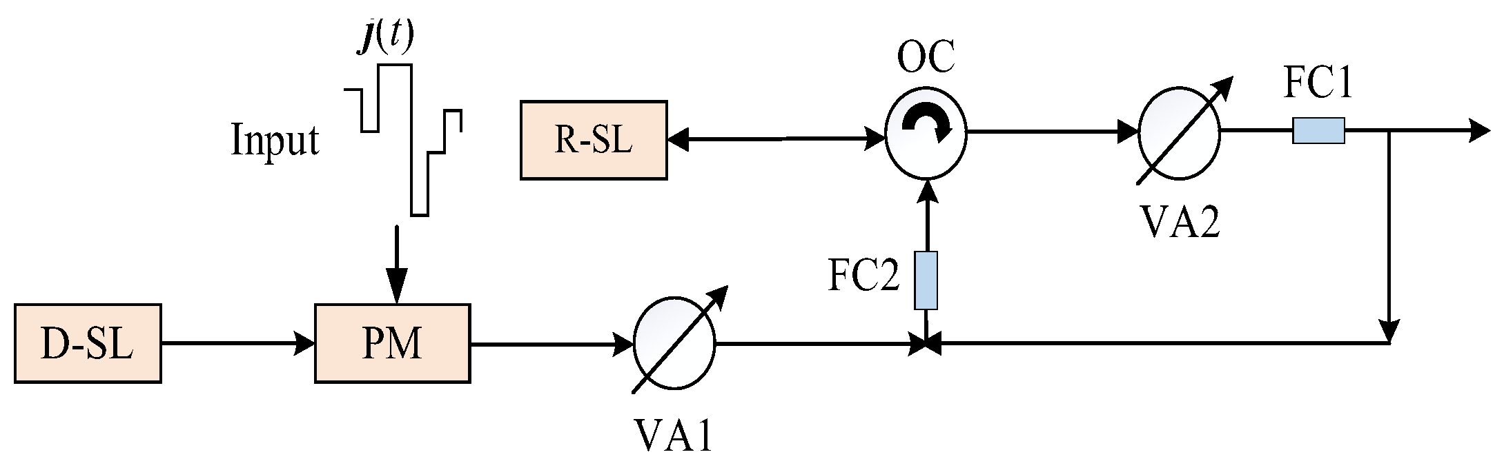
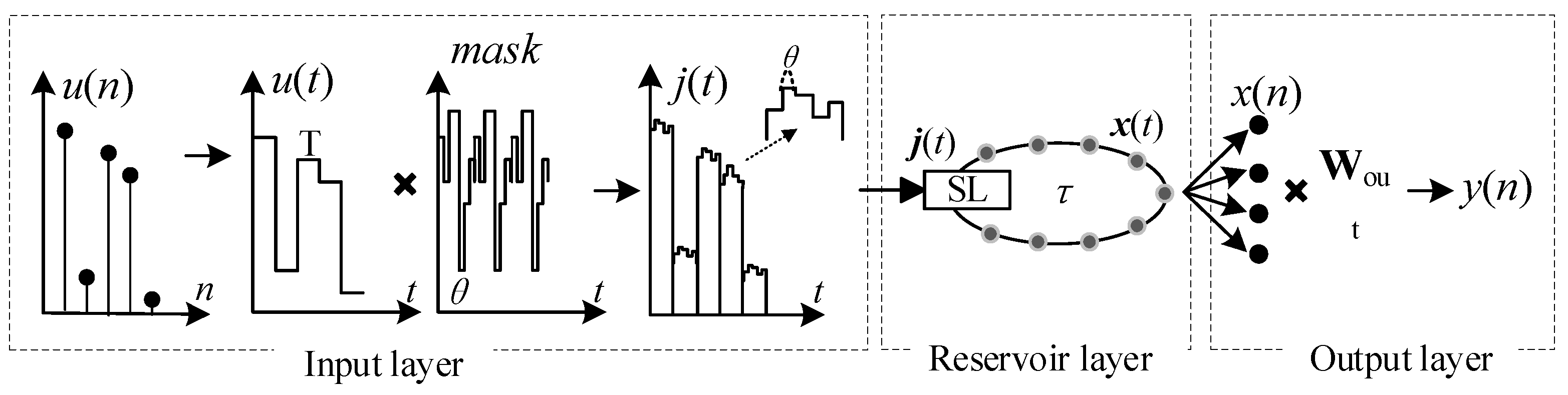
2. System Model
3. Results and Discussion
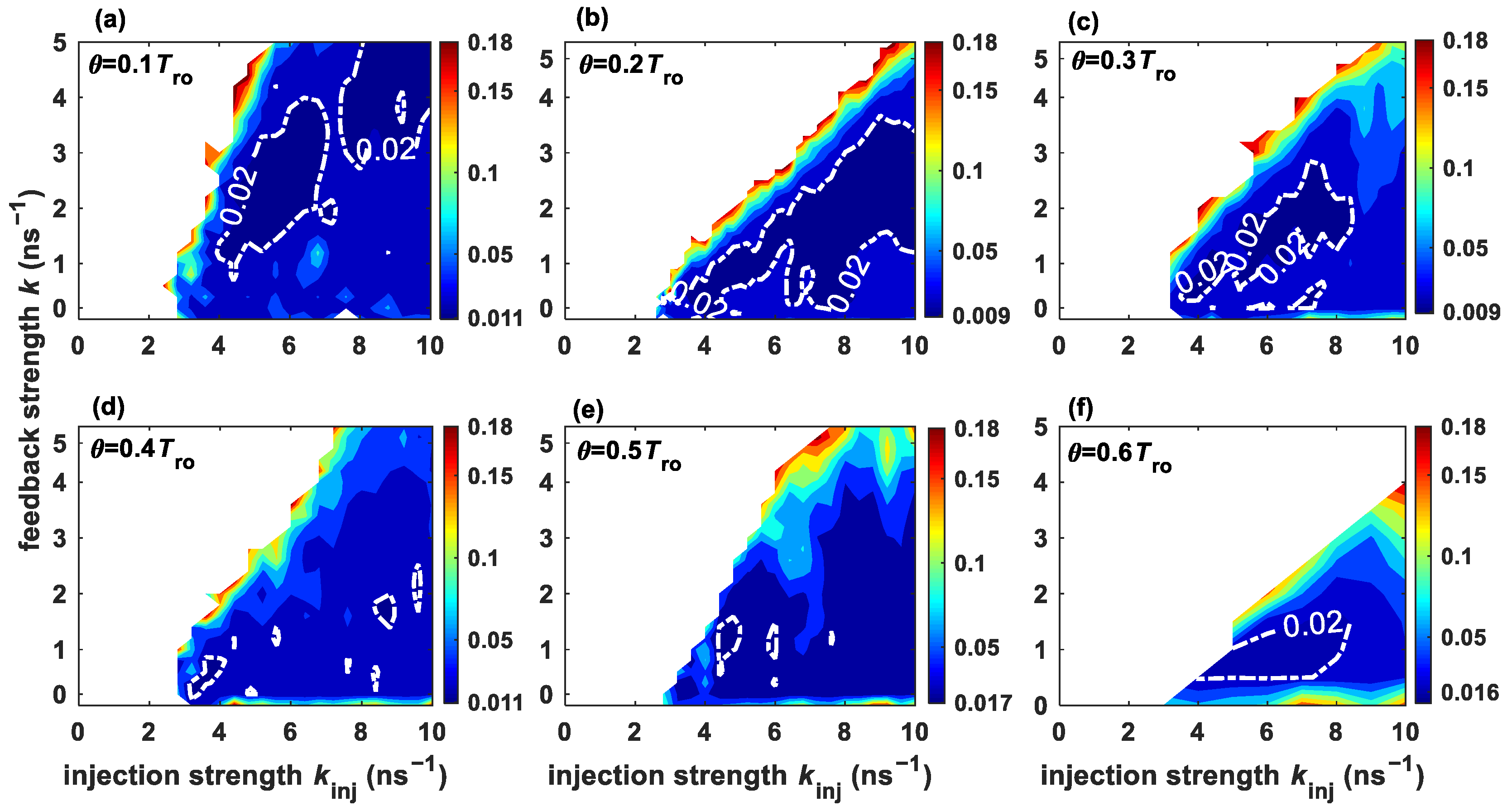
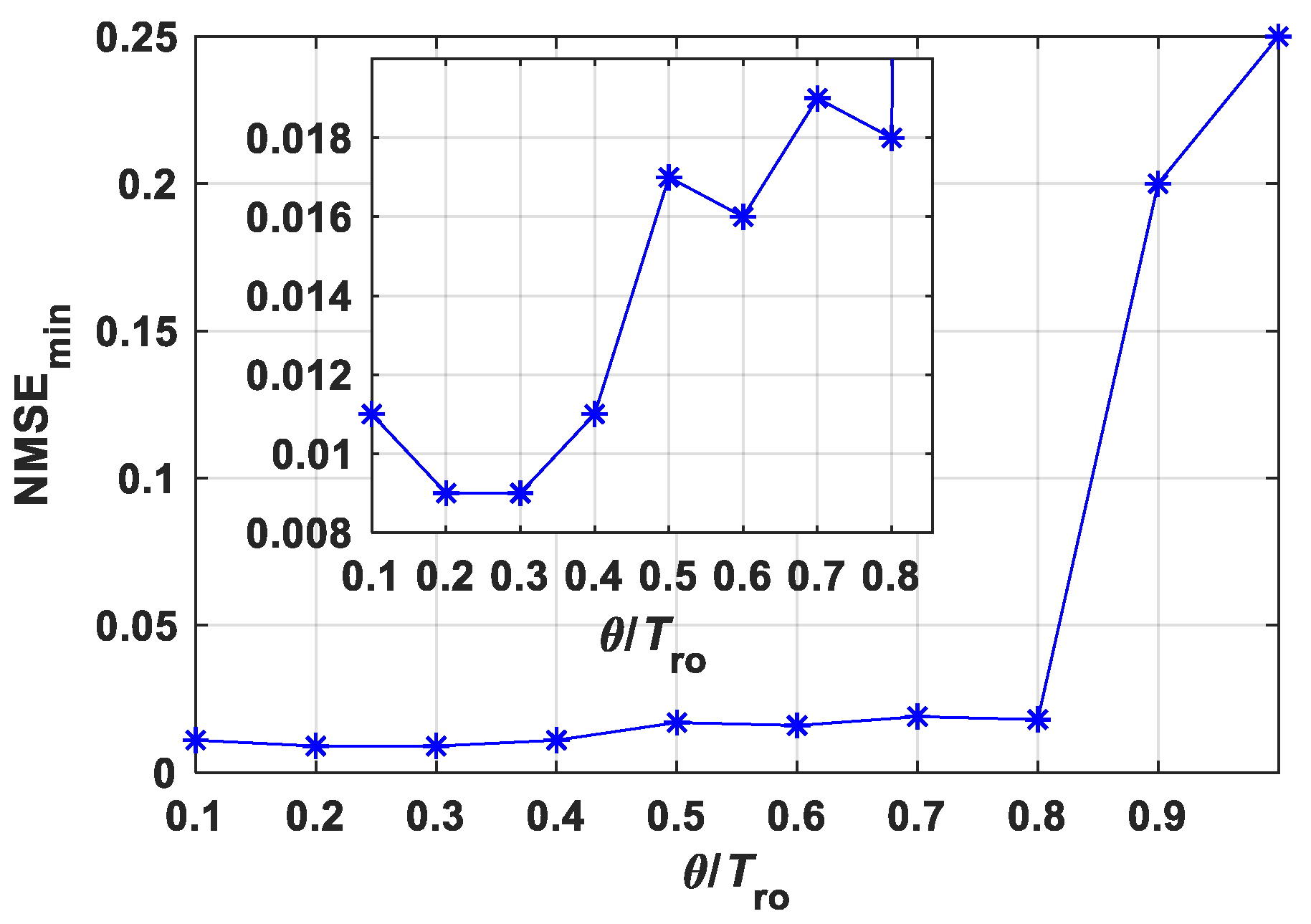
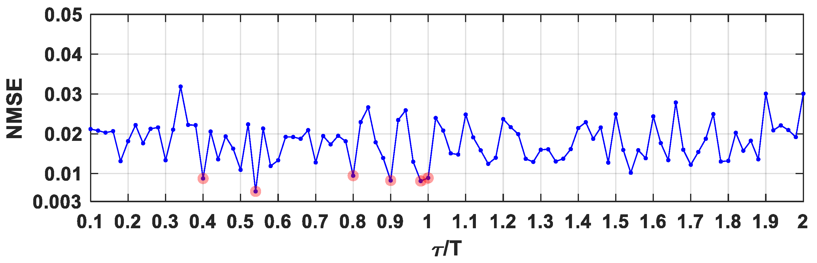
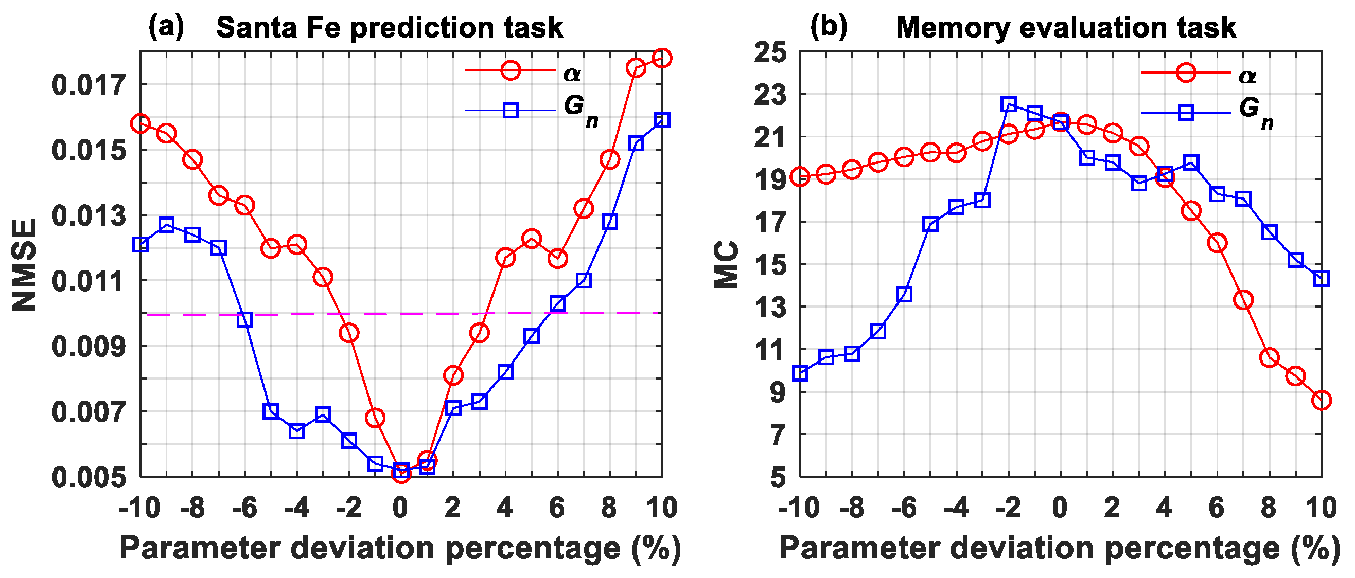
3.1. Santa Fe Time Series Prediction
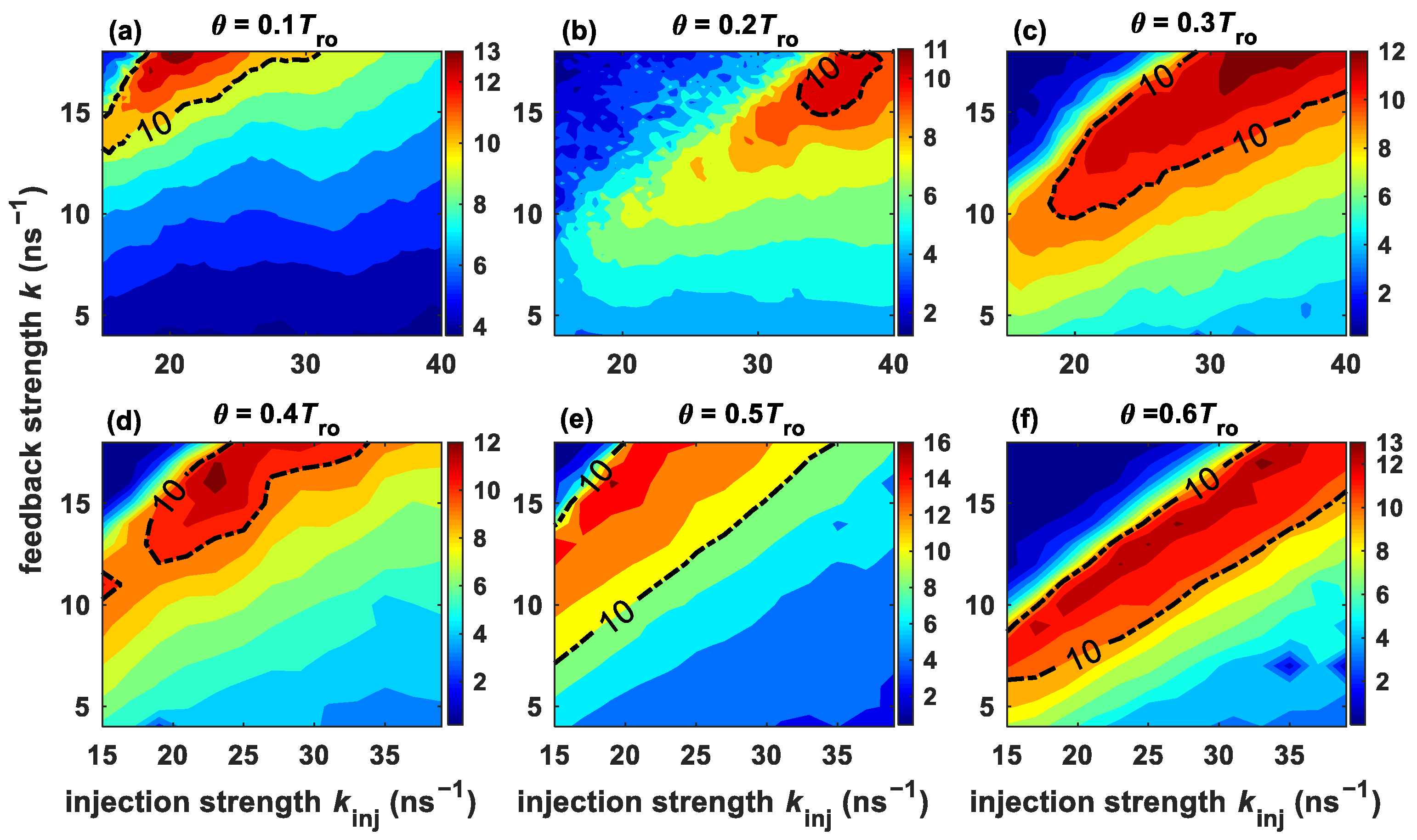
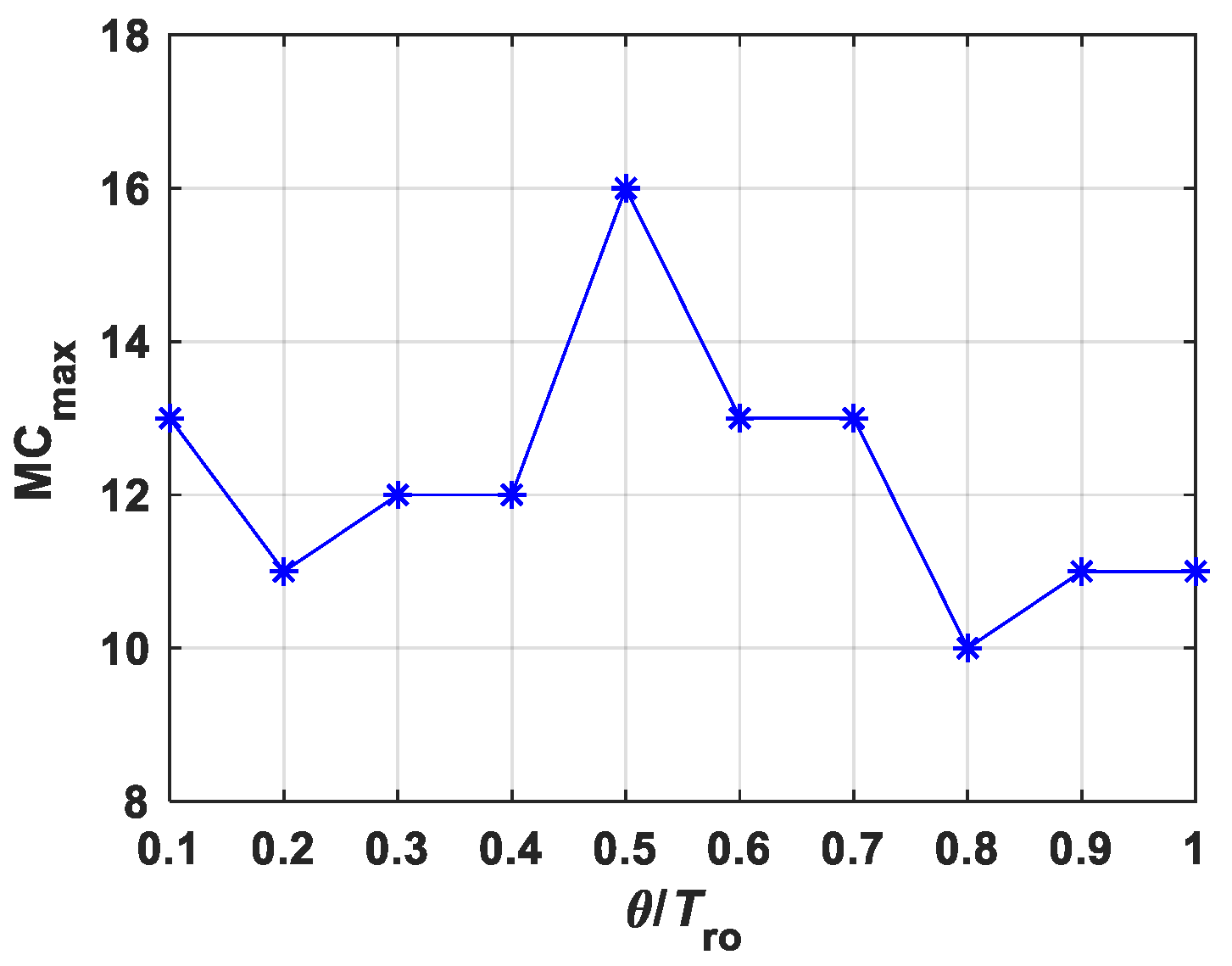
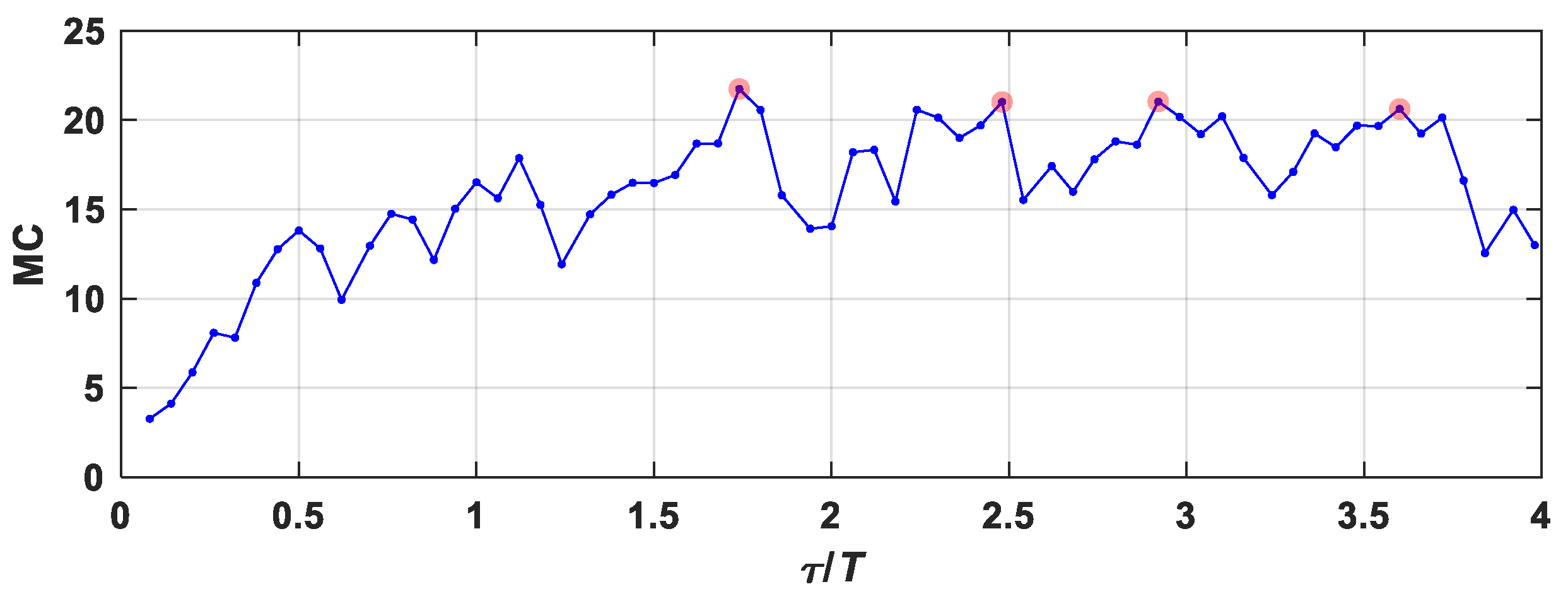
3.2. Memory Capacity Evaluation
3.3. Discussion
4. Conclusions
Author Contributions
Funding
Institutional Review Board Statement
Informed Consent Statement
Data Availability Statement
Conflicts of Interest
References
- Jaeger, H.; Haas, H. Harnessing nonlinearity: Predicting chaotic systems and saving energy in wireless communication. Science 2004, 304, 78–80. [Google Scholar] [CrossRef] [PubMed]
- Maass, W.; Natschläger, T.; Markram, H. Real-time computing without stable states: A new framework for neural computation based on perturbations. Neural Comput. 2002, 14, 2531–2560. [Google Scholar] [CrossRef] [PubMed]
- Verstraeten, D.; Schrauwen, B.; D’Haene, M.; Stroobandt, D. An experimental unification of reservoir computing methods. Neural Netw. 2007, 20, 391–403. [Google Scholar] [CrossRef]
- Soriano, M.C.; Brunner, D.; Escalona-Morán, M.; Mirasso, C.R.; Fischer, I. Minimal approach to neuro-inspired information processing. Front. Comput. Neurosci. 2015, 6, 68. [Google Scholar] [CrossRef] [PubMed]
- Kacper, P.; Ewelina, W.; Dawid, P.; Andrzej, B.; Agnieszka, P.; Vasileios, A.; Zoran, K.; Konrad, S. Molecules, semiconductors, light and information: Towards future sensing and computing paradigms. Coord. Chem. Rev. 2018, 365, 23–40. [Google Scholar]
- Gouhei, T.; Toshiyuki, Y.; Jean, B.; Ryosho, N.; Naoki, K.; Seiji, T.; Hidetoshi, N.; Daiju, N.; Akira, H. Recent advances in physical reservoir computing: A review. Neural Netw. 2019, 15, 100–123. [Google Scholar]
- Francesco, M.; Cristina, R.; Avishek, N.; Irene, M.; Darko, Z.; Marco, R.; Massimo, T. An overview on application of machine learning techniques in optical networks. IEEE Commun. Surv. Tutor. 2019, 21, 1383–1408. [Google Scholar]
- Kitayama, K.; Notomi, M.; Naruse, M.; Inoue, K.; Kawakami, S.; Uchida, A. Novel frontier of photonics for data processing—Photonic accelerator. APL Photonics 2019, 4, 090901. [Google Scholar] [CrossRef]
- Appeltant, L.; Soriano, M.C.; Van der Sande, G.; Danckaert, J.; Massar, S.; Dambre, J.; Schrauwen, B.; Mirasso, C.R.; Fischer, I. Information processing using a single dynamical node as complex system. Nat. Commun. 2011, 2, 468. [Google Scholar] [CrossRef]
- Cheng, T.Y.; Chou, D.Y.; Liu, C.C.; Chang, Y.J.; Chen, C.C. Optical neural networks based on optical fiber-communication system. Neurocomputing 2019, 364, 239–244. [Google Scholar] [CrossRef]
- Argyris, A.; Cantero, J.; Galletero, M.; Pereda, E.; Mirasso, C.R.; Fischer, I.; Soriano, M. Comparison of photonic reservoir computing system for fiber transmission equalization. IEEE J. Sel. Top. Quantum Electron. 2020, 26, 5100309. [Google Scholar] [CrossRef]
- Stelzer, F.; Röhm, A.; Lüdge, K.; Yanchuk, S. Performance boost of time-delay reservoir computing by non-resonant clock cycle. Neural Netw. 2020, 124, 158–169. [Google Scholar] [CrossRef] [PubMed]
- Ying, D.H.; Yanne, K.C. Classification of IO-modulated signals based on reservoir computing with narrowband optoelectronic oscillators. IEEE J. Quantum Electron. 2021, 57, 5000408. [Google Scholar]
- Jieru, S.; Jialin, M.; Chen, L.; Tianyu, W.; Changjin, W.; Hao, Z.; Qingqing, S.; David, W.; Lin, C. Self-powered optoelectronic synaptic device for both static and dynamic reservoir computing. Nano Energy 2025, 134, 110574. [Google Scholar]
- Larger, L.; Soriano, M.C.; Brunner, D.; Appeltant, L.; Gutierrez, J.M.; Pesquera, L.; Mirasso, C.R.; Fischer, I. Photonic information processing beyond Turing: An optoelectronic implementation of reservoir computing. Opt. Express 2012, 20, 3241–3249. [Google Scholar] [CrossRef]
- Duport, F.; Schneider, B.; Smerieri, A.; Haelterman, M.; Massar, S. All-optical reservoir computing. Opt. Express 2012, 20, 22783–22795. [Google Scholar] [CrossRef]
- Brunner, D.; Soriano Miguel, C.; Mirasso Claudio, R.; Fischer, I. Parallel photonic information processing at gigabyte per second data rates using transient states. Nat. Commun. 2013, 4, 1364. [Google Scholar] [CrossRef]
- Nguimdo, R.; Verschaffelt, G.; Danckaert, J.; Van der Sande, G. Simultaneous computation of two independent tasks using reservoir computing based on a single photonic nonlinear node with optical feedback. IEEE Trans. Neural Netw. Learn. Syst. 2015, 26, 3301–3307. [Google Scholar] [CrossRef]
- Hou, Y.S.; Xia, G.Q.; Yang, W.Y.; Wang, D.; Jayaprasath, E.; Jiang, Z.F.; Hu, C.X.; Wu, Z.M. Prediction performance of reservoir computing system based on a semiconductor laser subject to double optical feedback and optical injection. Opt. Express 2018, 26, 10211–10219. [Google Scholar] [CrossRef]
- Guo, X.; Xiang, S.; Zhang, Y.; Lin, L.; Wen, A.; Hao, Y. High-speed neuromorphic reservoir computing based on a semiconductor nanolaser with optical feedback under electrical modulation. IEEE J. Sel. Top. Quantum Electron. 2020, 26, 1500707. [Google Scholar] [CrossRef]
- Bogris, A.; Mesaritakis, C.; Deligiannidis, S.; Li, P. Fabry-Perot lasers as enablers for parallel reservoir computing. IEEE J. Sel. Top. Quantum Electron. 2021, 27, 7500307. [Google Scholar] [CrossRef]
- Zhong, D.Z.; Yang, H.; Xi, J.T.; Zeng, N.; Xu, Z.; Deng, F.Q. Predictive learning of multi-channel isochronal chaotic synchronization by utilizing parallel optical reservoir computers based on three laterally coupled semiconductor lasers with delay-time feedback. Opt. Express 2021, 29, 5279–5294. [Google Scholar] [CrossRef] [PubMed]
- Guo, X.; Zhou, H.; Xiang, S.; Yu, Q.; Zhang, Y.; Han, Y.; Wang, T.; Hao, Y. Short-term prediction for chaotic time series based on photonic reservoir computing using VCSEL with a feedback loop. Photon Res. 2024, 12, 1222–1230. [Google Scholar] [CrossRef]
- Hasegawa, H.; Kanno, K.; Uchida, A. Parallel and deep reservoir computing using semiconductor lasers with optical feedback. Nanophotonics 2023, 12, 869–881. [Google Scholar] [CrossRef] [PubMed]
- Qu, Y.; Lian, H.; Shao, R.; Liu, J.; Liu, L.; Yang, J. Time series analysis for financial indices using optical reservoir computing. Opt. Eng. 2024, 63, 054108. [Google Scholar] [CrossRef]
- Li, Z.; Xie, Y.; Xu, F.; Ye, Y.; Jiang, X.; Su, Y.; Li, L.; Chen, Z.; Tang, Y. Time-delayed reservoir computing using mutually coupled multimode semiconductor laser for high-speed image recognition. Opt. Laser Technol. 2025, 187, 112774. [Google Scholar] [CrossRef]
- Nguimdo, R.M.; Erneux, T. Enhanced performances of a photonic reservoir computer based on a single delayed quantum cascade laser. Opt. Lett. 2019, 44, 49–52. [Google Scholar] [CrossRef]
- Yang, Y.G.; Huang, Y.; Zhou, P.; Li, N.Q. Photonic reservoir computing for parallel task processing based on a feedback-free spin-polarized VCSEL. Opt. Commun. 2025, 574, 131225. [Google Scholar] [CrossRef]
- Harkhoe, K.; Verschaffelt, G.; Katumba, A.; Bienstman, P.; Van der Sande, G. Demonstrating delay-based reservoir computing using a compact photonic integrated chip. Opt. Express. 2020, 28, 3086–3096. [Google Scholar] [CrossRef]
- Cai, D.; Huang, Y.; Yang, Y.; Zhou, P.; Li, N. Enhanced performances of photonic reservoir computing using a semiconductor laser with random distributed optical feedback. Opt. Lett. 2023, 48, 6392–6395. [Google Scholar] [CrossRef]
- Zhu, P.J.; Wang, H.X.; Ji, Y.F. Performance enhancement reservoir computing system based on combination of VCESL optical feedback and mutual injection structure. IEEE J. Sel. Top. Quantum Electron. 2025, 31, 7400112. [Google Scholar] [CrossRef]
- Yamazaki, Y.; Kinoshita, K. Photonic physical reservoir computing with tunable relaxation time constant. Adv. Sci. 2024, 11, 2304804. [Google Scholar] [CrossRef] [PubMed]
- Yue, D.; Wu, Z.; Hou, Y.; Cui, B.; Jin, Y.; Dai, M.; Xia, G. Performance optimization research of reservoir computing system based on an optical feedback semiconductor laser under electrical information injection. Opt. Express. 2019, 27, 19931–19939. [Google Scholar] [CrossRef]
- Ortin, S.; Pesquera, L. Tackling the trade-off between information processing capacity and rate in delay-based reservoir computers. Front. Phys. 2019, 7, 210. [Google Scholar] [CrossRef]
- Ortin, S.; Pesquera, L. Reservoir computing with an ensemble of time-delay reservoirs. Cogn. Comput. 2017, 9, 327–336. [Google Scholar] [CrossRef]
- Rohm, A.; Ludge, K. Multiplexed networks: Reservoir computing with virtual and real nodes. J. Phys. Commun. 2018, 2, 085007. [Google Scholar] [CrossRef]
- Lang, R.; Kobayashi, K. External optical feedback effects on semiconductor injection laser properties. IEEE J. Quantum Electron. 1980, 16, 347–355. [Google Scholar] [CrossRef]
- Dejonckheere, A.; Duport, F.; Smerieri, A.; Fang, L.; Oudar, J.; Haelterman, M.; Massar, S. All-optical reservoir computer based on saturation of absorption. Opt. Express 2014, 22, 10868–10881. [Google Scholar] [CrossRef]
- Goldmann, M.; Köster, F.; Lüdge, K.; Yanchuk, S. Deep time-delay reservoir computing: Dynamics and memory capacity. Chaos. 2020, 30, 093124. [Google Scholar] [CrossRef]
- Estébanez, I.; Schwind, J.; Fischer, I.; Argyris, A. Accelerating photonic computing by bandwidth enhancement of a time-delay reservoir. Nanophotonics 2020, 9, 4163–4171. [Google Scholar] [CrossRef]
- Nakayama, J.; Kanno, K.; Uchida, A. Laser dynamical reservoir computing with consistency: An approach of a chaos mask signal. Opt. Express 2016, 24, 8679–8692. [Google Scholar] [CrossRef] [PubMed]
- Sugano, C.; Kanno, K.; Uchida, A. Reservoir computing using multiple lasers with feedback on a photonic integrated circuit. IEEE J. Sel. Top. Quantum Electron. 2020, 26, 1500409. [Google Scholar] [CrossRef]
Disclaimer/Publisher’s Note: The statements, opinions and data contained in all publications are solely those of the individual author(s) and contributor(s) and not of MDPI and/or the editor(s). MDPI and/or the editor(s) disclaim responsibility for any injury to people or property resulting from any ideas, methods, instructions or products referred to in the content. |
© 2025 by the authors. Licensee MDPI, Basel, Switzerland. This article is an open access article distributed under the terms and conditions of the Creative Commons Attribution (CC BY) license (https://creativecommons.org/licenses/by/4.0/).
Share and Cite
Li, Q.; Hou, Y.; Li, K.; Guo, X.; Hu, C.; Yue, D. Time Parameter Optimization for the Semiconductor Laser-Based Time-Delay Reservoir Computing System. Photonics 2025, 12, 455. https://doi.org/10.3390/photonics12050455
Li Q, Hou Y, Li K, Guo X, Hu C, Yue D. Time Parameter Optimization for the Semiconductor Laser-Based Time-Delay Reservoir Computing System. Photonics. 2025; 12(5):455. https://doi.org/10.3390/photonics12050455
Chicago/Turabian StyleLi, Qiudi, Yushuang Hou, Keqiang Li, Xiaoyu Guo, Chunxia Hu, and Dianzuo Yue. 2025. "Time Parameter Optimization for the Semiconductor Laser-Based Time-Delay Reservoir Computing System" Photonics 12, no. 5: 455. https://doi.org/10.3390/photonics12050455
APA StyleLi, Q., Hou, Y., Li, K., Guo, X., Hu, C., & Yue, D. (2025). Time Parameter Optimization for the Semiconductor Laser-Based Time-Delay Reservoir Computing System. Photonics, 12(5), 455. https://doi.org/10.3390/photonics12050455