DCNN–Transformer Hybrid Network for Robust Feature Extraction in FMCW LiDAR Ranging

Abstract

Frequency-Modulated Continuous-Wave (FMCW) Laser Detection and Ranging (LiDAR) systems are widely used due to their high accuracy and resolution. Nevertheless, conventional distance extraction methods often lack robustness in noisy and complex environments. To address this limitation, we propose a deep learning-based signal extraction framework that integrates a Dual Convolutional Neural Network (DCNN) with a Transformer model. The DCNN extracts multi-scale spatial features through multi-layer and pointwise convolutions, while the Transformer employs a self-attention mechanism to capture global temporal dependencies of the beat-frequency signals. The proposed DCNN–Transformer network is evaluated through beat-frequency signal inversion experiments across distances ranging from 3 m to 40 m. The experimental results show that the method achieves a mean absolute error (MAE) of 4.1 mm and a root-mean-square error (RMSE) of 3.08 mm. These results demonstrate that the proposed approach provides stable and accurate predictions, with strong generalization ability and robustness for FMCW LiDAR systems.

1. Introduction

With the rapid development of Laser Detection and Ranging (LiDAR) technology [1,2], Frequency-Modulated Continuous-Wave (FMCW) laser ranging systems [3,4] have gained considerable attention and been widely applied in autonomous driving [5], environmental monitoring [6], and topographic mapping [7], owing to their high-precision ranging capability. Unlike traditional Time-of-Flight (ToF) LiDAR systems [8], FMCW LiDAR achieves higher precision and a higher signal-to-noise ratio by continuously modulating the frequency of the transmitted laser, enabling not only accurate range detection [9] but also velocity estimation through Doppler-shift analysis [10].

During the FMCW ranging process, the transmitted signal and the target-reflected signal experience an optical path difference $\Delta L$. These two signals interfere within the interferometer to produce a beat-frequency signal $f_b$, whose characteristics are directly related to the target range R and relative velocity v. This relationship enables the extraction of critical ranging and velocity information. However, in practical scenarios, beat signals are often significantly degraded by various noise sources, making accurate detection and information extraction particularly challenging.

Traditional signal processing methods, such as Fourier Transform [11] and wavelet Transform [12], provide basic processing of FMCW signals. Several studies have proposed enhanced ranging algorithms based on spectral analysis. For instance, some approaches combine frequency and phase estimation of the beat signal to improve distance measurement accuracy [13,14]. Kamata et al. developed a compact photonic-crystal-based phase shifter for I/Q modulators, enabling efficient generation of carrier-suppressed single-sideband signals with a side-mode suppression ratio of 22.3 dB [15]. Cheng et al. introduced a correlation-coefficient criterion based on differential terms to select effective intrinsic mode functions, and combined singular value decomposition (SVD) with wavelet denoising, thereby improving the signal-to-noise ratio from 5.28 dB to 21.06 dB [16]. Wang et al. proposed a WT-VMD algorithm integrating the sparrow search algorithm (SSA) with variational mode decomposition (VMD), which increased the signal-to-noise ratio by 138.5% and reduced the root-mean-square error by 81.8% in simulated signal processing [17].

In recent years, deep learning has demonstrated substantial potential in signal processing [18], particularly through architectures such as Convolutional Neural Networks (CNNs) and Transformers. With strong capabilities in feature extraction and pattern modeling, these models have achieved notable success in diverse fields, including image processing [19], speech recognition [20], and time-series signal analysis [21].

Building on these advances, researchers have increasingly applied deep learning to FMCW radar ranging tasks to overcome the limitations of traditional spectral analysis methods. For example, Park et al. [22] proposed a five-layer neural network utilizing features derived from Fast Fourier Transform (FFT), which substantially reduced distance estimation errors. Sang et al. [23] introduced a CNN-based framework for sparse signal processing that preserved high velocity-estimation accuracy even under partial data loss. More recently, Cho et al. [24] developed a lightweight one-dimensional CNN with a frequency-shift reuse mechanism, enabling accurate distance estimation with minimal labeled data and reduced hardware costs. Collectively, these studies underscore the advantages of deep learning in FMCW radar applications, particularly in enhancing accuracy, robustness, and adaptability under challenging conditions.

However, most existing studies focus on radar-based implementations or hybrid approaches that still depend on handcrafted spectral features, while end-to-end deep learning solutions for FMCW LiDAR distance prediction remain limited. To bridge this gap, we propose a feature extraction and prediction framework that integrates the complementary strengths of Deep Convolutional Neural Networks (DCNNs) and Transformer architectures (DT model). The model directly learns discriminative representations from FMCW LiDAR beat signals, enabling robust and accurate distance estimation under complex backgrounds and high-noise conditions.

2. Methodology

2.1. DCNN for Local Spectral Feature Extraction

In FMCW LiDAR, the target range is traditionally estimated by applying Fast Fourier Transform (FFT) to convert the beat-frequency signal into the frequency domain and locating its dominant spectral peak. While FFT-based methods provide a straightforward mapping from spectral peaks to distance, they are inherently limited in capturing subtle patterns such as side lobes, noise fluctuations, and multi-target interference across the full spectrum. Convolutional Neural Networks (CNNs) are widely adopted in deep learning due to two key properties: local connectivity and weight sharing. To leverage these properties for spectral analysis, a one-dimensional CNN (1D-CNN) is employed to automatically learn and extract discriminative spectral features. By sliding convolutional kernels along the frequency axis, the 1D-CNN identifies local spectral signatures, suppresses noise, and aggregates multi-scale patterns indicative of the target range. This deep convolutional feature extractor forms the first stage of our hybrid architecture, enabling robust local representation of beat-frequency information before global modeling with the Transformer encoder.

Building on the conventional 1D-CNN, we further design two parallel convolutional branches with complementary functions at the front end of the network to simultaneously capture both coarse-grained and fine-grained features of the beat-frequency signals. This dual-branch structure enhances the network’s capacity to model multi-scale spectral representations, which is essential for robust feature extraction under diverse signal conditions.

The complete architecture of the proposed DT model is illustrated in Figure 1.

In the large-kernel branch, the first layer applies a one-dimensional convolution (Conv1d) with a kernel size of $18\times 1$ and a stride of 2 for downsampling, aiming to capture global pulse trends over a wide temporal window. This is followed by one-dimensional batch normalization (BatchNorm1d) and a learnable activation function (MetaAconC). A subsequent Conv1d layer with a kernel size of $10\times 1$ and a stride of 2 is then used to extract mid-scale features. To mitigate overfitting, a dropout layer (Dropout, $p=0.2$) is introduced, followed by a one-dimensional max pooling layer (MaxPool1d) that further aggregates the extracted features to yield the final output of this branch.

In the fine-grained branch, the spectrum is sequentially processed by four one-dimensional convolutional layers with kernel size $6\times 1$, two with stride 1 and two with stride 2, while the channel dimensions evolve from 1 to 50, 40, 30, and finally 30. Each convolution is followed by batch normalization and MetaAconC activation, with a dropout layer ($p=0.2$) applied after the last stride-2 convolution. To progressively adjust the temporal resolution, max pooling (kernel size 2, stride 2) is inserted after the second and fourth convolutions, producing the final output feature map of this branch.

After downsampling both branches to the same temporal scale, their outputs are fused through element-wise multiplication across both the channel and time dimensions, generating multi-scale coupled features.

The proposed DCNN feature extractor thus combines two complementary pathways: a large-kernel branch that captures coarse global trends across the entire beat-frequency spectrum, and a fine-grained branch that models detailed local spectral patterns. By fusing these representations through element-wise multiplication, the network constructs a richly descriptive multi-scale embedding of the FMCW beat signal. This fusion not only enhances the discrimination of true peaks from artifacts but also improves robustness to interference, thereby providing stable local features for the subsequent Transformer stage.

2.2. Integrating the Transformer into the DT Model

The Transformer model [25], renowned for its strong modeling capacity, has achieved remarkable success in long-sequence learning tasks, and is particularly effective in capturing complex temporal dependencies in sequential data [26]. Central to the Transformer architecture is the self-attention mechanism, which computes dependencies across all positions within a sequence. This mechanism captures relationships among sequence elements through a weighted summation, where the weights are adaptively determined attention scores.

We introduce the self-attention mechanism underlying the Transformer Block as preliminaries. Specifically, given an input sequence $\mathbf{X}=\{x_1,x_2,\dots ,x_n\}$, where $x_i$ represents the input vector at the ith position, the attention mechanism can be calculated as follows:

$$\mathrm{Attention}(\mathbf{Q},\mathbf{K},\mathbf{V})=\mathrm{softmax}\left({\displaystyle \frac{\mathbf{Q}{\mathbf{K}}^T}{\sqrt{d_k}}}\right)\mathbf{V}$$

(1)

where $\mathbf{Q}$, $\mathbf{K}$, and $\mathbf{V}$ denote the query, key, and value matrices, respectively, and $d_k$ is the dimensionality of the key vectors. This formulation describes how the attention weights are computed via the dot product between the query and key matrices, and how these weights are used to perform a weighted summation over the value matrix, thereby capturing the relationships and dependencies across different positions in the sequence.

To further enhance the model’s representation capability, the Transformer architecture incorporates a multi-head attention mechanism. Multi-head attention divides the query, key, and value matrices into h separate groups, computes attention independently within each group, and then concatenates the results. Assuming that the dimensionality of the queries, keys, and values in each head is $d_k$, the multi-head attention can be formulated as

$$\mathrm{MultiHead}(\mathbf{Q},\mathbf{K},\mathbf{V})=\mathrm{Concat}({\mathrm{head}}_1,{\mathrm{head}}_2,\dots ,{\mathrm{head}}_h){\mathbf{W}}^O$$

(2)

where each attention head is calculated as

$${\mathrm{head}}_i=\mathrm{Attention}(\mathbf{Q}{\mathbf{W}}_i^Q,\mathbf{K}{\mathbf{W}}_i^K,\mathbf{V}{\mathbf{W}}_i^V)$$

(3)

The multi-head attention mechanism enables the model to attend to information from different positions simultaneously, which is essential for global reasoning over the features extracted by the DCNN.

Following multi-scale feature fusion, the resulting tensor is reshaped into a sequence of frequency-bin embeddings and input to a Transformer encoder for global spectral modeling. In our implementation, the fused feature map is first augmented with positional encodings to preserve spectral ordering, and then passed through stacked self-attention and position-wise feedforward networks, each wrapped by residual connections and layer normalization.

By attending across all frequency positions, the Transformer captures long-range correlations and contextual dependencies that extend beyond the local receptive fields of convolutional kernels. This global attention mechanism highlights informative spectral peaks, suppresses noise artifacts, and resolves closely spaced returns that may otherwise be indistinguishable. The enriched, context-aware representation produced by the Transformer is subsequently flattened and passed to fully connected layers for distance regression.

Specifically, the output feature sequence from the Transformer encoder is flattened into a one-dimensional vector, which is then processed by two fully connected layers: the first reduces dimensionality, and the second generates the final distance estimation. In this way, the integration of the Transformer endows the proposed DT model with both local feature sensitivity and global spectral reasoning, thereby achieving improved robustness and accuracy in FMCW LiDAR ranging under real-world noise and interference conditions.

3. Method Implementation

3.1. Experimental Setup

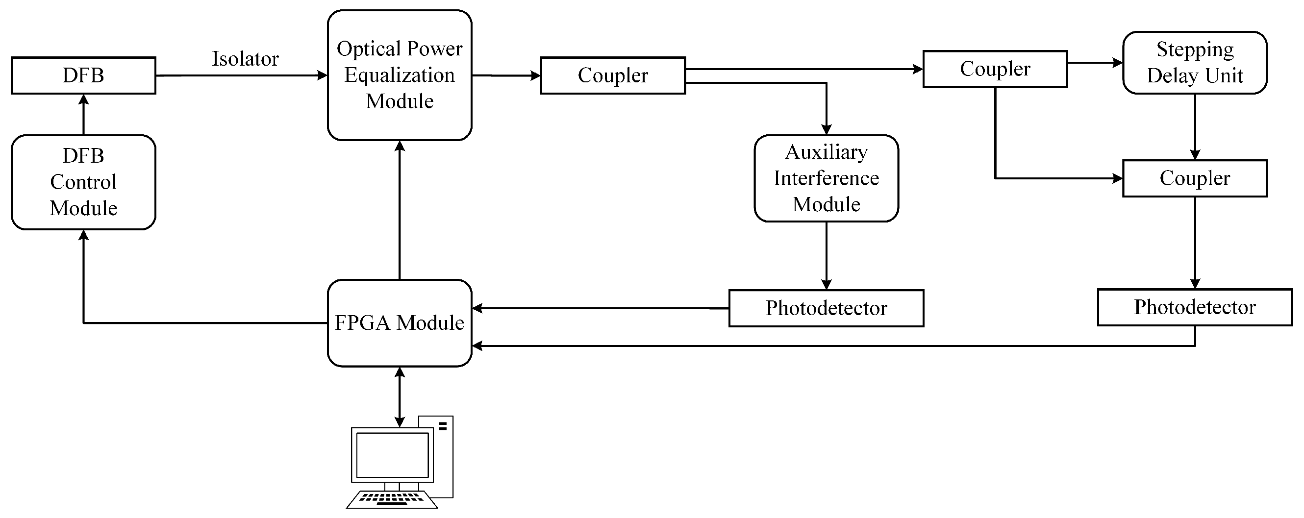
The experimental setup of the proposed FMCW LiDAR ranging system is designed to validate the performance of the developed algorithm under realistic conditions. The overall structure of the system is illustrated in Figure 2.

As the core of the system, a distributed feedback (DFB) semiconductor laser operates at a central wavelength of 1550 nm. The DFB control module provides both current and temperature regulation, ensuring stable wavelength tuning and precise frequency modulation. Specifically, the current driver supplies a bias current for continuous-wave operation, as well as a modulation current to achieve the FMCW frequency chirp, while a temperature controller is used to suppress wavelength drift. The DFB output passes through an optical isolator to prevent back-reflections and is subsequently fed into an Optical Power Equalization Module, which compensates for power fluctuations and stabilizes the output intensity.

The equalized signal is split by an optical coupler into two paths. The light in one path is directed into the Auxiliary Interference Module and then detected by a photodetector. This branch provides real-time monitoring of the frequency chirp and reference signals, which are processed by the FPGA module for system calibration and compensation. The other path is used for ranging. The light propagates through an additional coupler into a Stepping Delay Unit that emulates the round-trip propagation of the reflected signal. By adjusting the delay steps, equivalent target distances can be simulated with high accuracy. The delayed signal is recombined via another coupler and subsequently converted into an electrical beat signal by a second photodetector.

All detected signals are then digitized and processed in the FPGA module, which interfaces with a host computer for data acquisition, algorithm validation, and real-time control. This architecture ensures accurate signal emulation, stable laser operation, and flexible ranging scenarios for testing the proposed deep learning-based distance estimation algorithm.

3.2. Dataset Construction

The raw data used in this study were obtained from the FMCW laser ranging system described above. In this system, a Frequency-Modulated Continuous-Wave signal is transmitted, and the echo reflected from the target is mixed with a local oscillator to generate a beat-frequency signal, from which the target distance can be extracted.

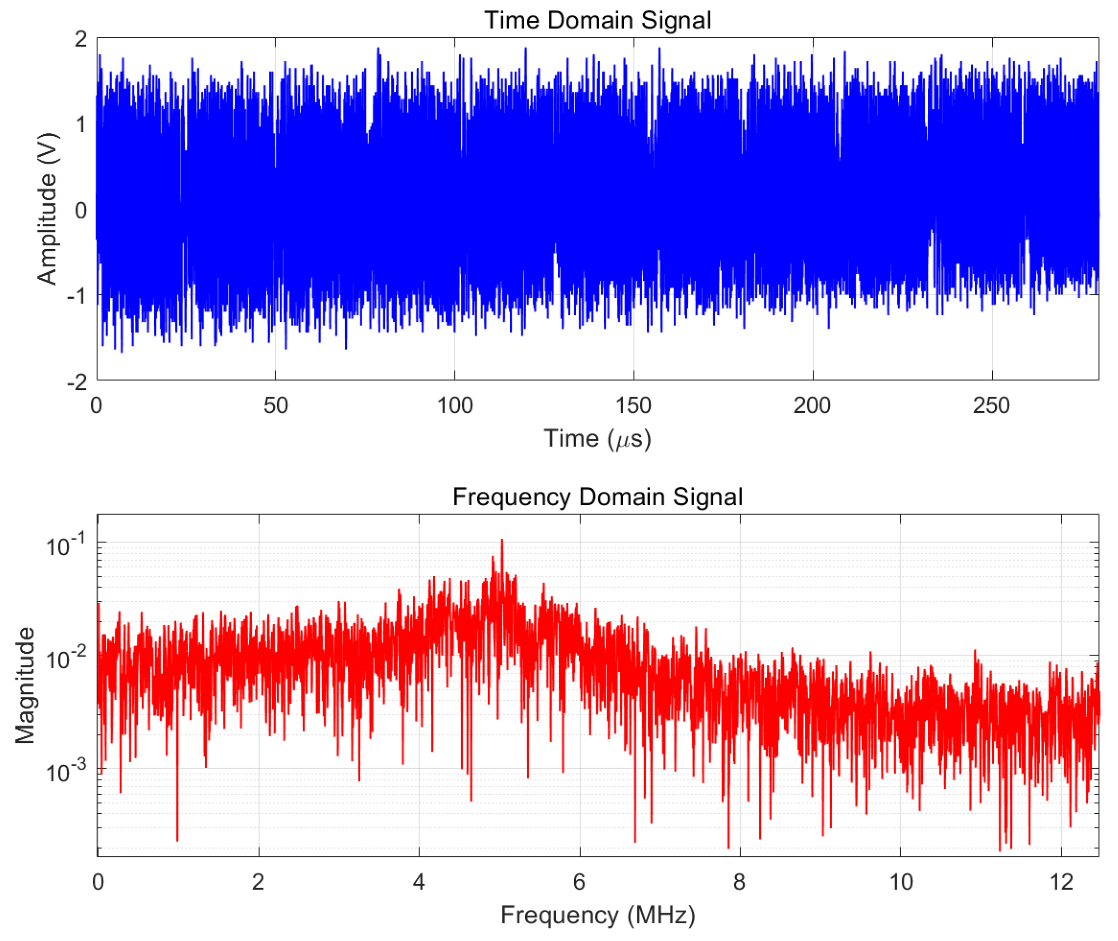
Figure 3 presents an example of the raw signal acquired from the FMCW system. The signal inherently contains multiple noise sources originating from the laser, photodetector, and electronic circuits. This example corresponds to a target distance of approximately 5 m, where the beat frequency is centered around 5 MHz. As the ranging distance increases, the frequency spectrum undergoes noticeable broadening, which becomes the dominant source of interference. Under such conditions, the signal-to-noise ratio (SNR) falls below 5 dB, complicating reliable signal extraction. When the distance is further extended, this spectral broadening becomes even more severe, leading to continued SNR degradation.

To construct the dataset, beat-frequency signals were collected at 64 target distances ranging from 3 m to 40 m. Each sample was transformed into the frequency domain and represented as a $1\times 4096$ vector. Standard preprocessing procedures, including windowing and zero-padding, were applied to maintain spectral resolution and amplitude fidelity. These spectral representations inherently encode both target distance and reflectivity.

This dataset forms the basis for training the proposed deep learning model. It not only enables robust distance estimation under low-SNR conditions but also provides a quantitative benchmark for evaluating deep learning–based signal analysis methods in practical FMCW LiDAR systems.

3.3. Network Model Training

During the training process, the Smooth L1 Loss function [27] is employed as the regression loss for the proposed model. The loss function is defined as follows:

$${\mathrm{Smooth}}_{L1}\left(x\right)=\left\{\begin{array}{cc}0.5x^2,\hfill & \mathrm{if}\left|x\right|<1\hfill \\ \left|x\right|-0.5,\hfill & \mathrm{otherwise}\hfill \end{array}\right.$$

where x represents the error between the predicted value and the ground truth, i.e., $x=\widehat{y}-y$. When the error $\left|x\right|$ is less than 1, the loss adopts a squared error form (similar to L2 loss), which emphasizes the precise fitting of small errors. When the error $\left|x\right|$ is greater than or equal to 1, the loss switches to an absolute error form (similar to L1 loss), avoiding excessive penalization of large errors.

Compared with the traditional Mean-Squared Error (MSE), Smooth L1 Loss applies a linear penalty for large residuals ($\left|x\right|\ge 1$), improving robustness to outliers, while retaining a quadratic penalty for small residuals ($\left|x\right|<1$), and Smooth L1 Loss enables fine fitting of minor variations in the signal.

This balanced design allows the model to achieve an effective trade-off between accuracy and robustness, particularly improving performance when dealing with noisy signals and datasets containing outliers.

Table 1. Training procedure of DT model.

Step	Procedure	Step	Procedure
1	Load dataset	13	Validation phase
2	Dataset preprocessing	14	• Disable gradient computation
3	Data splitting (Train/Val/Test)	15	• Forward pass and loss on validation set
4	Model parameter initialization	16	• Record validation loss
5	Main Loop	17	Testing phase
6	Training phase	18	• Disable gradient computation
7	• Gradient management	19	• Forward pass and loss on test set
8	• Forward computation	20	• Record test loss
9	• Loss calculation	21	Learning rate adjustment
10	• Backpropagation	22	Layer freezing/optimizer reconfiguration
11	• Loss accumulation	23	Early stopping counter control
12	• Training loss recording	24	Loop Termination

summarizes the distance inversion procedure based on our DT model.

3.4. Hyperparameter Optimization

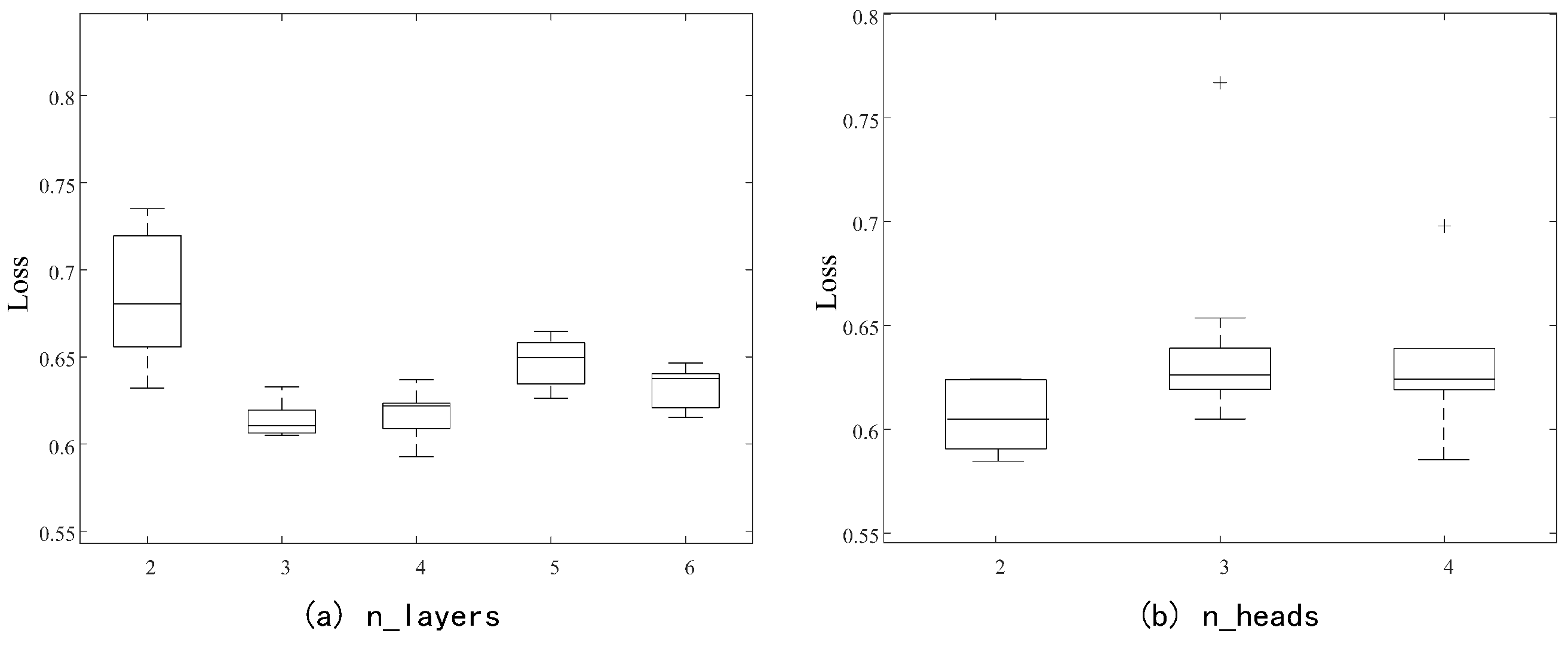
Figure 4a illustrates the effect of Transformer layer depth on model performance. Here, the number of layers denotes the count of stacked Transformer modules, each comprising (1) a self-attention mechanism that computes dependencies among positions in the input sequence to produce weighted feature representations, and (2) a feedforward neural network that applies nonlinear transformations to the self-attention outputs. Each additional layer learns progressively more abstract representations of the input data. Consequently, the choice of layer depth directly impacts model capacity and performance.

When the model uses two layers, the median performance metric is 0.68 but with a wide distribution, reflecting substantial fluctuations and unstable training. Increasing the depth to three or four layers slightly reduces the median metric while narrowing the distribution, indicating lower variability and improved stability. With five layers, the median metric decreases further to 0.66, but the distribution broadens again, suggesting diminished stability. At six layers, the median performance drops to 0.64, though the distribution becomes narrower, representing the smallest fluctuations and the most stable training. Overall, deeper architectures improve stability but provide limited accuracy gains beyond three layers. Thus, a three-layer configuration is selected as the optimal balance between accuracy and stability.

Figure 4b presents the influence of the number of attention heads on model performance. The number of heads corresponds to the parallel attention sublayers applied to the input, enabling the model to attend to different feature subspaces simultaneously. While self-attention captures dependencies across sequence positions, multi-head attention expands this capacity by learning diverse feature representations.

With two heads, the median loss is approximately 0.61, accompanied by a wide interquartile range (IQR), indicating high variability. Increasing the number of heads to three raises the median loss slightly to 0.62 but narrows the distribution, implying more stable yet less accurate performance. At four heads, the median loss remains similar to that at three heads, though outliers persist and loss values remain relatively high. The best performance—the lowest median loss with the narrowest IQR—is achieved with two heads, suggesting that additional heads neither improve accuracy nor enhance stability, and may even degrade performance.

3.5. Training Strategies

In this study, several training strategies are adopted to enhance efficiency, improve stability, and mitigate overfitting. Specifically, we employ learning rate scheduling, partial parameter freezing, and early stopping. Each strategy is implemented with a distinct purpose, and together they contribute to more effective training and improved generalization performance.

3.5.1. Learning Rate Scheduling

The learning rate is a crucial hyperparameter in neural network training. An excessively high learning rate may lead to unstable optimization, whereas an overly low rate can result in slow convergence or entrapment in local minima. To address this, we adopt a dynamic adjustment strategy in which a scheduler automatically modifies the learning rate based on the validation loss, thereby balancing convergence speed and training stability.

Specifically, the scheduler monitors the validation loss at the end of each training epoch and adjusts the learning rate accordingly. When the loss decreases, the scheduler lowers the learning rate to enable finer parameter updates in later stages of training. Conversely, when the loss remains high, a relatively larger learning rate is preserved to accelerate convergence. This adaptive mechanism promotes rapid convergence in the early phase while ensuring gradual refinement in subsequent stages, thereby mitigating the risk of premature convergence to suboptimal solutions.

3.5.2. Partial Parameter Freezing

To mitigate overfitting and reduce unnecessary computational overhead during certain stages of training, a partial parameter freezing strategy was employed. Once the validation loss dropped below $1\times {10}^{-4}$, selected layers were frozen and excluded from backpropagation. This reduces the model’s degrees of freedom, thereby improving training stability and efficiency. By constraining less critical components of the network, the remaining parameters can concentrate on learning task-relevant features, further enhancing model effectiveness.

Following the freezing step, we adopted AdamP [28], an adaptive optimizer with decoupled weight decay, to refine the training of the unfrozen parameters. This optimizer improves generalization while avoiding redundant computations, allowing the model to allocate its capacity toward optimizing critical components, which ultimately boosts training efficiency and performance.

3.5.3. Early Stopping

To prevent overfitting and preserve generalization performance on the validation set, an early stopping mechanism was employed. The key idea is to terminate training if the validation loss fails to exhibit meaningful improvement over a predefined number of epochs, thereby avoiding redundant computation.

In this study, early stopping was activated once the validation loss fell below $5\times {10}^{-4}$. The mechanism continuously monitored loss variations, and if no substantial improvement was observed within a specified epoch window, training was halted. This strategy not only mitigates the risk of overfitting but also reduces computational overhead.

After extensive hyperparameter tuning, the optimal model configuration was determined, as summarized in

Table 2. Hyperparameter list of DT model.

Hyperparameter Name	Value
Maximum Training Epochs	5000
Batch Size	32
Learning Rate	0.00001
Dropout Rate	0.2
Number of Transformer Layers	3
Number of Transformer Heads	2
Dimension of Q, K, and V	256
Network Freezing Threshold	0.0001
Early Stopping Patience	200

. This configuration achieves low test loss while maintaining a favorable trade-off between performance and computational cost, underscoring the efficiency of the proposed approach.

3.6. Experimental Results and Analysis

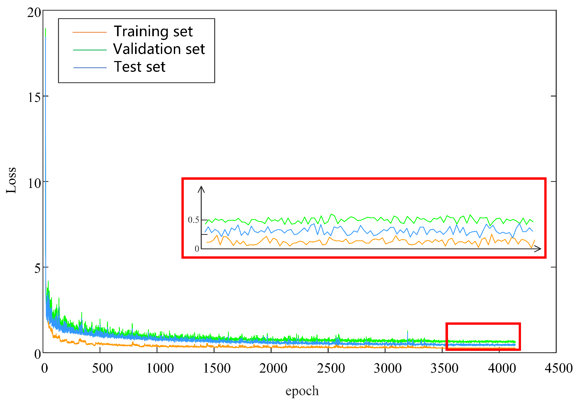
Figure 5 depicts the loss trajectories of the proposed DT model. During the initial training epochs, the loss decreased rapidly across all datasets, indicating that the model quickly adapted to the data and captured essential patterns. As training progressed, the rate of loss reduction gradually plateaued, suggesting that the model had approached convergence and was nearing optimal performance.

The validation and test loss curves remain closely aligned throughout training, indicating consistent performance across datasets and the absence of significant overfitting. In the later epochs, both validation and test losses remain low and stable, with no noticeable increase, further confirming the model’s robust generalization capability.

The inset panel provides a magnified view of fine-grained fluctuations in the loss curves between approximately epochs 3800 and 4200. During this period, minor discrepancies among training, validation, and test losses are observed, further indicating stable and well-generalized learning. Overall, the experimental results demonstrate that the model consistently achieves strong performance across all datasets without signs of overfitting. The model initially learns rapidly and then gradually stabilizes, producing low and consistent loss values on both the validation and test sets, which reflects its robust generalization capability.

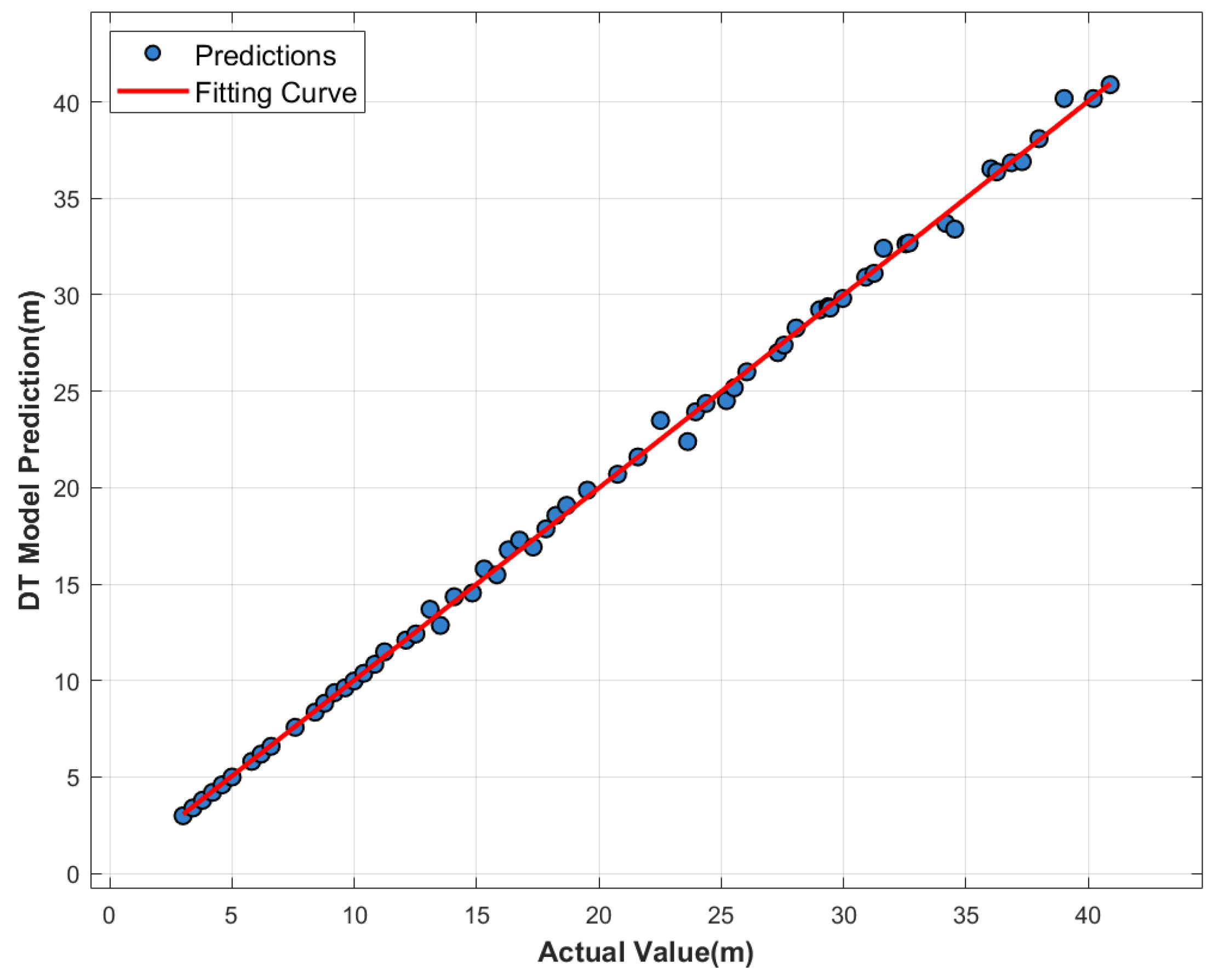
In Figure 6, the blue dots represent the distance predictions of the DT model, with the x-axis corresponding to the true values and the y-axis to the predicted distances. Ideally, all points should lie along the diagonal line where the predicted and true distances are equal. The red curve represents a second-order polynomial fitted to the predicted points, capturing the overall prediction trend. The blue points exhibit a clear linear distribution along this fitted curve. Across the prediction range of 3–40 m, the points are evenly distributed around the fitted curve, indicating consistent stability throughout the measurement range. The positive slope of the fitted curve, closely aligned with the 45-degree reference line, confirms that the model effectively captures the positive correlation between true and predicted distances.

Most predictions closely match the ground truth, demonstrating high accuracy and reliable performance across the full measurement range. Notably, even at the extremities of the distance spectrum—both minimum and maximum—the predictions remain smooth and consistent, without abrupt deviations. This underscores the model’s robustness and stability in handling signals with widely varying amplitude levels.

For comparison, we also apply a traditional FFT-based spectral estimation method based on the same dataset. In the short-range regime (distances below approximately 7 m), the traditional method achieves performance comparable to that of our proposed model, with ranging errors within 3 mm. However, as the distance increases, the signal quality degrades, and the limitations of the traditional approach become apparent. At around 15 m, the ranging error already exceeds 80 mm, and beyond 20 m, the method is unable to provide reliable distance estimates. In contrast, our DCNN–Transformer model consistently maintains millimeter-level accuracy across the entire measurement range (3–40 m), even under low-SNR conditions.

Quantitatively, the model achieves a mean absolute error (MAE) of just 4.1 mm and a root-mean-square error (RMSE) of 3.08 mm on the test set. Notably, the model also performs exceptionally well in the long-distance range (30–40 m), demonstrating the effectiveness of multi-scale convolution in spatial feature extraction, and the Transformer’s capability in modeling long-range temporal dependencies via self-attention. Overall, the synergistic effect of the DCNN and Transformer not only improves the efficiency of feature extraction from the signal but also enhances noise suppression on complex backgrounds, offering robust support for high-precision ranging in FMCW LiDAR systems under diverse application scenarios.

4. Conclusions

In this study, we proposed a novel deep learning-based framework to address the limitations of FMCW LiDAR systems in high-precision distance measurement. By integrating the complementary strengths of the DCNN and Transformer architectures, the signal-processing capabilities of FMCW LiDAR were substantially enhanced. Specifically, the DCNN extracts multi-scale spatial features through stacked depthwise and pointwise convolutions, thereby improving spectral representation. Simultaneously, the Transformer’s self-attention mechanism effectively models temporal dependencies within beat-frequency sequences, capturing long-range correlations with high fidelity.

The experimental results validated the effectiveness and robustness of the proposed DT model. The training process exhibited rapid convergence, with stable loss trajectories on both the validation and test sets, indicating minimal overfitting. The quantitative evaluations further demonstrated that the model delivers highly accurate, millimeter-level distance predictions across a wide measurement range while maintaining strong generalization even in long-distance scenarios. These findings highlight the potential of the proposed approach for enabling high-precision and robust distance estimation in practical FMCW LiDAR applications.

We also discussed the model’s generalization and the limitations of the present work. In our experiments, the maximum tested range was 40 m due to current laboratory constraints, and all measurements were performed in an optical-fiber-based setup. Consequently, we do not claim empirical validation beyond this range or in free-space conditions at this stage. Nevertheless, there are several reasons to expect the proposed architecture to generalize to more challenging scenarios. The DCNN’s multi-scale feature extraction is well suited to capturing spectral broadening associated with increased ranging distance, while the Transformer’s ability to model long-range dependencies helps maintain coherent estimation when beat-frequency sequences become more complex. These intrinsic properties, combined with the model’s stability up to 40 m, warrant further investigation into extended-range and in situ deployments.

To validate and enhance the model’s generalization, we will further explore our work through both experimental and algorithmic approaches. Experimentally, we plan to extend the measurement range beyond 40 m and transition from fiber-based tests to free-space field trials, covering a variety of target reflectivities, motion states (static and dynamic targets), multi-target scenarios, and environmental conditions (e.g., different SNR regimes, atmospheric turbulence, and temperature variations). Algorithmically, we will explore targeted techniques such as physics-informed loss functions, synthetic long-range data augmentation, and domain-adaptation and transfer-learning strategies to bridge the gap between laboratory and field domains, as well as uncertainty quantification methods (e.g., predictive intervals or Bayesian approximations) to provide confidence estimates for each prediction. We will also investigate robustness-oriented training methods (such as adversarial/noise augmentation), ensemble methods, and lightweight model compression methods (including quantization/pruning) to facilitate real-time deployment on embedded platforms.

In summary, the proposed DCNN–Transformer framework significantly enhances distance estimation accuracy and robustness in FMCW LiDAR under the tested conditions. Although the current validation is limited to fiber-based measurements up to 40 m, planned extensions—both in measurement campaigns and in methodological refinements—are expected to rigorously evaluate and further enhance the model’s generalization to longer-range and real-world operational scenarios.