Robust and Interpretable Machine Learning for Network Quality Prediction with Noisy and Incomplete Data

Abstract

Accurate classification of optical communication signal quality is crucial for maintaining the reliability and performance of high-speed communication networks. While existing supervised learning approaches achieve high accuracy on laboratory-collected datasets, they often face difficulties in generalizing to real-world conditions due to the lack of variability and noise in controlled experimental data. In this study, we propose a targeted data augmentation framework designed to improve the robustness and generalization of binary optical signal quality classifiers. Using the OptiCom Signal Quality Dataset, we systematically inject controlled perturbations into the training data including label boundary flipping, Gaussian noise addition, and missing-value simulation. To further approximate real-world deployment scenarios, the test set is subjected to additional distribution shifts, including feature drift and scaling. Experiments are conducted under 5-fold cross-validation to evaluate the individual and combined impacts of augmentation strategies. Results show that the optimal augmentation setting (flip_rate = 0.10, noise_level = 0.50, missing_rate = 0.20) substantially improve robustness to unseen distributions, raising accuracy from 0.863 to 0.950, precision from 0.384 to 0.632, F1 from 0.551 to 0.771, and ROC-AUC from 0.926 to 0.999 compared to model without augmentation. Our research provides an example for balancing data augmentation intensity to optimize generalization without over-compromising accuracy on clean data.

1. Introduction

1.1. Background

Optical communication systems form the backbone of modern digital infrastructure, enabling high-capacity, low-latency data transmission across long distances [1,2]. With the continuously growing demand from users for optical communication systems [3], assessing and ensuring the integrity and performance of transmitted signals has become a significant challenge. Traditional performance monitoring relies on hardware signal quality measurements [4], expert analysis, and even user feedback, which result in high costs, time consumption, limited scalability, and slow response times.

In recent years, machine learning (ML) has emerged as a promising alternative for automated optical signal quality classification [5,6,7]. Leveraging labeled datasets collected from laboratory setups, ML-based approaches can rapidly infer the state of a communication link based on a set of signals and environmental parameters [8]. However, laboratory datasets are often collected under controlled conditions, meaning they lack the variability, noise, and unpredictability inherent in real-world deployment environments. Consequently, models trained exclusively on clean laboratory data tend to overfit [9] to idealized conditions and exhibit substantial performance drops when exposed to real-world data that contain sensor noise, environmental fluctuations, missing measurements, and parameter drift.

A critical component of this study is the OptiCom Signal Quality Dataset, which serves as the foundation for our experiments. The dataset contains 586 samples (538 good, 47 poor), each of which contains 20 performance metrics of optical communication signals. Data collection combined controlled laboratory experiments with field measurements in operational optical communication networks, using instruments such as optical power meters, spectrum analyzers, and bit-error-rate (BER) testers.

Preliminary analysis shows that a small subset of features, including transmission distance, distance between, and fiber attenuation, can readily separate the two quality classes. While this enables high accuracy in clean data regimes, it also risks encouraging classifiers to rely on overly simplistic and brittle decision rules, limiting their ability to generalize to the complex and noisy conditions of real-world deployments. This observation highlights the need for data augmentation strategies that deliberately introduce uncertainty and variability into the training process, thereby guiding models to learn more robust and generalizable decision boundaries.

1.2. Research Questions

Building on this observation, this work proposes a targeted data augmentation and distribution shift simulation framework to improve the robustness of optical signal quality classifiers. The framework systematically evaluates how different augmentation strategies affect model generalization under realistic conditions, while also providing interpretability analysis through feature importance assessments. This study is guided by the following research questions:

• How can augmentation strategies (e.g., label boundary flipping, Gaussian noise injection, missing-value simulation) be designed to reflect plausible real-world variations?
• How do different augmentation strategies and intensities affect the generalization of classifiers when exposed to distribution shifts (e.g., feature drift and scaling)?
• To what extent can interpretability analysis (via SHAP) provide insights into model stability and the operational significance of influential features?

1.3. Contributions

To address the above questions, this paper makes the following contributions:

• We develop a targeted data augmentation framework that introduces label flipping, Gaussian noise, and synthetic missing values to mimic real-world uncertainties in optical networks.
• We propose an evaluation protocol that explicitly incorporates test-time distribution shifts (scaling and additive drift), enabling deployment-aware robustness assessment.
• We conduct systematic evaluations across multiple ML models under various perturbation settings and provide interpretability analysis via SHAP to reveal the stability and importance of key features.
• Our findings offer practical guidelines on how much perturbation can be introduced to balance robustness and clean-data performance.

1.4. Limitations

Despite its potential benefits, the proposed approach has several limitations. First, the experiments rely primarily on the OptiCom Signal Quality Dataset. This dataset offers the advantage of encompassing a wide range of physical-layer and environmental parameters (e.g., transmission distance, fiber attenuation, temperature, and humidity). In addition to laboratory measurements, it also contains field data collected from operational optical networks. Nevertheless, the absence of multi-source or large-scale real-world datasets may limit the generalizability of the conclusions.

Second, the augmentation techniques employed in this study (e.g., Gaussian noise variance, boundary definitions for label flipping, drift magnitude) were manually set based on domain expertise and exploratory analysis. While this design enables controlled evaluation, it may not yield optimal or universally applicable settings. Furthermore, the modeling of sensor drift at test time relies mainly on uniform scaling and additive feature shifts, which offer only an abstraction of real-world degradation mechanisms. More complex drift patterns (e.g., correlated feature shifts, nonlinear interactions, or seasonal variations) remain unaddressed.

By acknowledging these limitations, we provide a clear scope for this study while identifying directions for future work. These include validating the framework on datasets collected from diverse operational networks, automating augmentation parameter selection, and extending the approach to incorporate more sophisticated drift models and more diverse model architectures.

2. Related Work

Machine learning (ML) methods have been widely applied to quality-of-transmission (QoT) estimation in optical networks [10]. For example, Sartzetakis et al. combined a physical-layer model (PLM) with ML algorithms to improve QoT prediction accuracy [11], while Kozdrowski et al. employed Random Forest and XGBoost models on dense wavelength-division multiplexing (DWDM) optical networks, achieving advanced predictive performance [12]. However, these approaches largely overlook the risk of overfitting to clean data obtained under controlled scenarios, underscoring the need for techniques that enhance robustness under real-world deployment conditions.

In the broader ML literature, data augmentation has emerged as a key strategy to improve robustness and mitigate overfitting [13]. Established techniques include SMOTE for addressing class imbalance [14] and KNN [15] or MICE [16] for missing-value imputation. Augmentation strategies based on Gaussian noise injection [17] and synthetic label noise [18] have also been shown to produce more resilient models. Although most of these studies focus on computer vision and natural language processing, the underlying principle—introducing realistic perturbations during training to improve generalization—applies directly to the task of optical signal classification.

3. Methods

This study explored targeted data augmentation strategies to simulate real-world imperfections and thereby enhance the robustness of machine learning models for optical signal quality classification. All experiments were conducted on the OptiCom Signal Quality Dataset, which contains multiple physical-layer and environmental parameters (e.g., transmission distance, fiber attenuation, temperature, humidity) along with corresponding signal quality labels (good/poor). Exploratory data analysis (EDA) revealed that certain features (such as transmission distance and fiber attenuation) exhibited strong class-separating capability within specific ranges, enabling near-perfect binary classification without the need for additional features. While advantageous under controlled laboratory conditions, such separability would reduce generalization when noise, missing values, and distribution shifts are present in real-world deployments. To address this, we designed a processing pipeline that systematically introduces realistic perturbations during both training and evaluation.

3.1. Data Processing and Augmentation Pipeline

The order of preprocessing and augmentation was carefully designed to reflect realistic data acquisition and processing steps. Discrete features and labels were first converted into numerical format via one-hot encoding. Gaussian noise was then injected into the raw feature space of $X\_\mathrm{train}$ to emulate sensor measurement errors. Next, random missing values were introduced into $X\_\mathrm{train}$ at a specified rate, followed by imputation. After these perturbations, features were normalized, and $X\_\mathrm{test}$ was transformed using the scaler fitted on the training data. Label noise was then introduced into $y\_\mathrm{train}$ to model annotation uncertainty near decision boundaries. Finally, class imbalance was addressed using SMOTE oversampling on $X\_\mathrm{train}$ and $y\_\mathrm{train}$.

The overall procedure is summarized in Figure 1, which visually outlines each processing and augmentation stage from raw data to model training and evaluation.

3.2. Gaussian Noise

Measurement noise was simulated by adding Gaussian perturbations to each feature: $X^{\prime }=X+\mathcal{N}(0,{\sigma }_f)$ where ${\sigma }_f=\mathrm{noise}\_\mathrm{level}\times \mathrm{std}\left(X_f\right)$ is scaled to each feature’s standard deviation. We experimented with noise levels $\{0.00,0.05,0.10,0.20,0.30,0.50,0.75,1.00\}$. This formulation preserves the relative variability across features while maintaining realistic noise magnitudes. Models trained on noise-augmented data were evaluated on the unperturbed test set to study robustness under varying noise intensities.

3.3. Missing Value

To emulate incomplete measurements caused by hardware faults or incomplete reporting, missing values were inserted at random feature positions with different rates $\{0.00,0.05,0.10,0.20,0.30,0.50\}$. Imputation was then applied using three different strategies—mean imputation, k-nearest neighbors (KNN with $k=5$), and multivariate imputation by chained equations (MICE)—to compare their impact on model performance.

3.4. Label Perturbation

Label noise was introduced in a structured manner to reflect realistic misclassification patterns. Instead of a uniform flip rate, the probability of flipping a label depended on whether the sample lay within predefined "decision boundary" intervals identified via EDA, where multiple individual features could independently separate the classes. Samples falling into more such boundaries were assigned higher flip probabilities, reflecting the intuition that borderline or overly separable points in laboratory data are more error-prone in real settings.

Let c be the number of boundaries hit by sample i. Given a base flip rate $\alpha$, the flip probability is computed as

$$p_{\mathrm{flip}}=1-{(1-\alpha )}^c.$$

We also evaluated a linear scaling of flip probability with c. Base flip rates tested were $\alpha \in \{0.01,0.05,0.10,0.15,0.20,0.35,0.50\}$. The full set of boundary intervals were: Transmission Distance (18–19), Distance Between (3–4), Fiber Attenuation (0.08–0.09), Splice Losses (0.16–0.18), Optical Amplifier Gain (8–9), PMD Coefficient (0.03–0.04), CD Coefficient (0.01–0.02), Temperature (23–24), and Humidity (58–59).

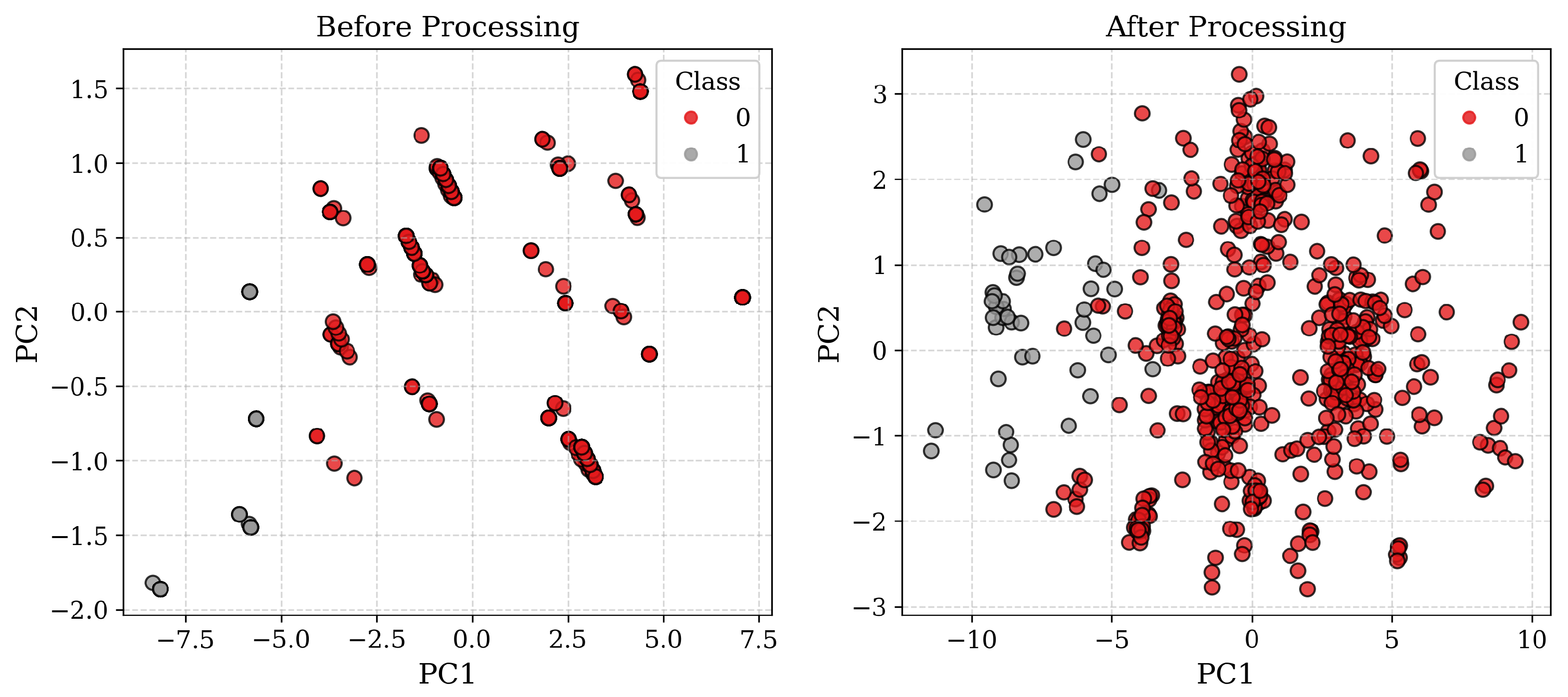
3.5. PCA Visualization of Data Before and After Processing

To illustrate the effect of preprocessing and augmentation on feature space structure, we applied Principal Component Analysis (PCA) to project the data into two dimensions. Figure 2 shows the scatter plots for the original dataset and the augmented dataset, with class labels indicated by color. Clear changes in distribution and overlap are visible, reflecting the intended perturbations.

3.6. Training, Testing, and Evaluation Scheme

Each experiment employed five machine learning algorithms: Random Forest [19], XGBoost [20], LightGBM [21], Support Vector Machine (SVM) [22], and Naïve Bayes. All models used default parameters. All experiments used 5-fold cross-validation with a fixed random seed ($\mathrm{SEED}=42$). To determine whether augmentations improved generalization, the test set remained unmodified ($y\_\mathrm{test}$ unperturbed) during ablation experiments. Each augmentation type was tested independently, then with grid search over hyperparameters to identify combinations that maintained performance while improving robustness.

For the final combined evaluation, all augmentation techniques (applied at reduced intensities) were introduced to $X\_\mathrm{test}$ and $y\_\mathrm{test}$. In addition, two perturbation types were incorporated to reflect deployment-related variability: (i) feature scaling, achieved by multiplying features by random factors drawn from a uniform range, to emulate calibration mismatches between laboratory setups and field equipment; (ii) additive shifts, applied as fixed offsets to feature values, to represent gradual environmental influences and equipment aging effects over time.

3.7. Metrics and Model Interpretability

Performance was evaluated using accuracy, precision, recall, F1 score, and ROC-AUC. Mean and standard deviation across folds are also reported.

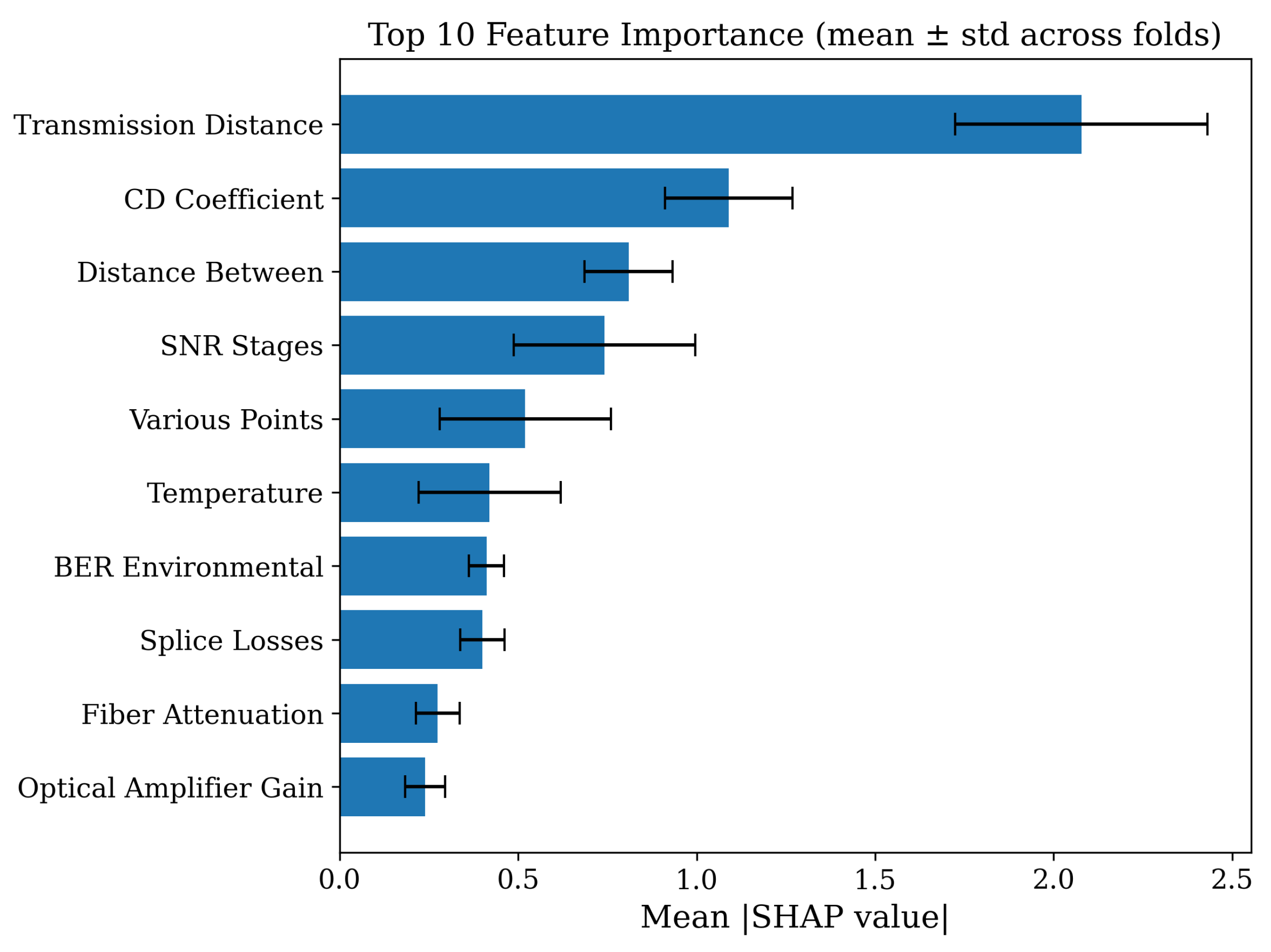
To interpret the models and identify influential features, SHAP [23] values were computed for each test sample in each fold of the best-performing model. SHAP values were then averaged across folds to estimate each feature’s overall contribution, with standard deviations indicating consistency of influence. The top-10 features by mean SHAP value were visualized in bar plots (with error bars for standard deviation) and in beeswarm plots to show per-sample SHAP value distributions.

4. Results

4.1. Label Flip Robustness

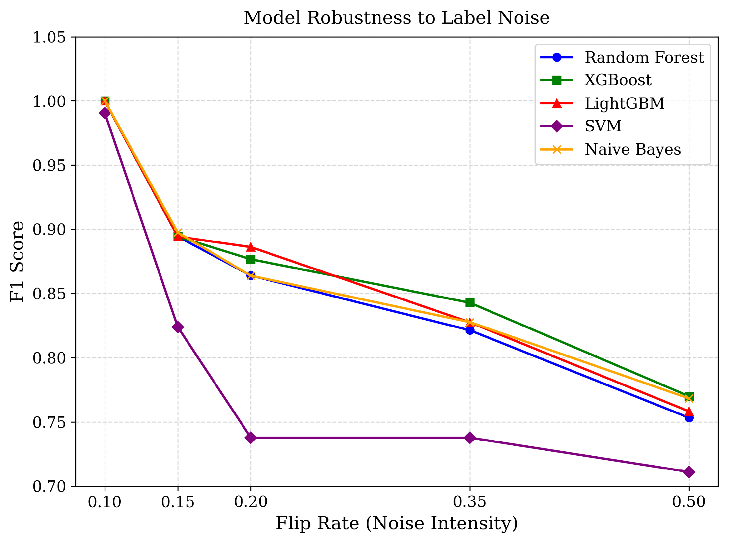
Figure 3 and

Table 1. Model F1 score under varying label flip rates.

Flip Rate	Random Forest	XGBoost	LightGBM	SVM	Naïve Bayes
0.10	1.000	1.000	1.000	0.990	1.000
0.15	0.894	0.894	0.894	0.824	0.897
0.20	0.864	0.877	0.886	0.738	0.864
0.35	0.821	0.843	0.828	0.738	0.828
0.50	0.753	0.770	0.758	0.711	0.768

show the F1 score degradation for various controlled label flip rates ($\alpha$) across models. All models achieved near-perfect F1 score at $\alpha =0.10$, indicating strong resilience to low-level annotation noise. However, performance declined progressively as flip rates increased. Tree-based models (Random Forest, XGBoost, LightGBM) maintained relatively stable performance up to $\alpha =0.20$, whereas SVM exhibited earlier and sharper degradation beyond $\alpha =0.15$. At $\alpha =0.50$, F1- core fell to around 0.75–0.77 for most models, reflecting the difficulty of learning from highly corrupted labels.

This difference in robustness can be attributed to the mechanisms of these algorithms. Ensemble tree methods aggregate decisions over multiple feature subspaces, effectively averaging out localized noise, while margin-based SVM is more sensitive to boundary-localized mislabels. Notably, LightGBM demonstrated slightly better tolerance than Random Forest under moderate flip rates, highlighting the benefit of gradient-boosting optimization. These findings suggest that, for deployment in noisy labeling environments, tree-based ensembles are the most reliable, while SVM may require additional noise-handling strategies.

4.2. Gaussian Noise Robustness

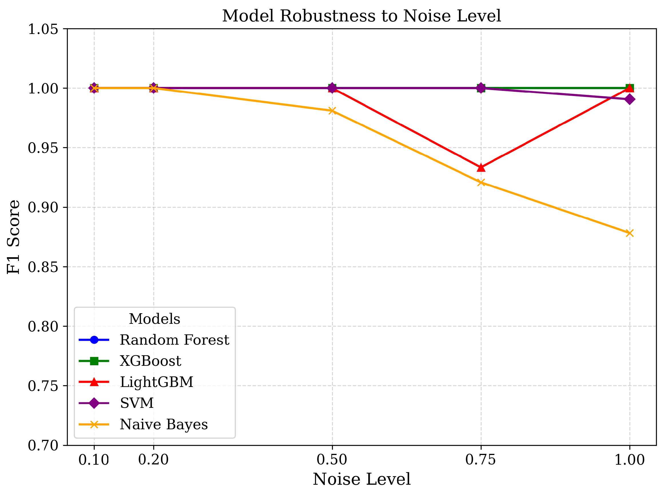
Figure 4 and

Table 2. Model F1 score under varying Gaussian noise levels.

Noise Rate	Random Forest	XGBoost	LightGBM	SVM	Naïve Bayes
0.10	1.000	1.000	1.000	1.000	1.000
0.20	1.000	1.000	1.000	1.000	1.000
0.50	1.000	1.000	1.000	1.000	0.981
0.75	1.000	1.000	0.933	1.000	0.921
1.00	1.000	1.000	1.000	0.990	0.878

illustrate model robustness to Gaussian feature perturbations. For noise levels up to $\sigma =0.50$, all models retained near-perfect accuracy, indicating that their learned decision boundaries generalized well to moderate measurement noise. Beyond this threshold, Naïve Bayes exhibited measurable degradation, with F1 score dropping to around 0.88 at $\sigma =1.00$. This heightened sensitivity can be attributed to its strong reliance on probabilistic distributional assumptions: Gaussian noise substantially distorts feature distributions, and the multiplicative nature of likelihood estimation amplifies such deviations.

In contrast, ensemble tree models (Random Forest, XGBoost, LightGBM) and SVM maintained stable performance even under heavy noise, suggesting that class separability in the feature space remainws largely intact. Interestingly, LightGBM showed a slight dip at $\sigma =0.75$ relative to Random Forest and XGBoost, hinting that its boosting-based feature splits may be somewhat more vulnerable to extreme perturbations. Overall, ensemble methods demonstrated the strongest generalization, while Naïve Bayes proved least suited for deployment in scenarios with high sensor variance.

4.3. Missing-Value Robustness

To evaluate robustness under incomplete measurements, we compared three imputation methods: mean, KNN, and MICE. As shown in

Table 3. Naïve Bayes F1 score under different imputation methods.

Missing Rate	Mean	KNN	MICE
0.10	0.873	1.000	1.000
0.20	0.744	1.000	1.000
0.35	0.711	1.000	1.000
0.50	0.613	0.897	0.981

, mean imputation resulted in rapid performance degradation for Naïve Bayes, with F1 scores dropping to ≈0.61 at 50% missingness. KNN imputation performed better, maintaining high F1 scores up to 35% missingness but showed noticeable decline at the 50% level. In contrast, MICE consistently preserved multivariate feature relationships and delivered near-perfect F1 scores even at the highest missing rate (≈0.981 for Naïve Bayes). Across models, MICE provided the most stable recovery of missing values and was therefore adopted as the default imputation strategy in subsequent experiments.

Table 4. Model F1 score under under varying missing rates (mean imputation).

Missing Rate	Random Forest	XGBoost	LightGBM	SVM	Naïve Bayes
0.10	1.000	1.000	1.000	0.990	0.873
0.20	1.000	0.990	0.990	0.972	0.744
0.35	0.990	0.990	0.990	0.812	0.711
0.50	0.972	0.936	1.000	0.747	0.613

,

Table 5. Model F1 score under under varying missing rates (KNN imputation).

Missing Rate	Random Forest	XGBoost	LightGBM	SVM	Naïve Bayes
0.10	1.000	0.990	0.990	1.000	1.000
0.10	1.000	0.990	0.990	1.000	1.000
0.10	1.000	1.000	1.000	1.000	1.000
0.50	0.981	0.990	0.990	0.948	0.897

and

Table 6. Model F1 score under under varying missing rates (MICE imputation).

Missing Rate	Random Forest	XGBoost	LightGBM	SVM	Naïve Bayes
0.10	1.000	0.990	0.990	1.000	1.000
0.20	1.000	1.000	0.990	1.000	1.000
0.35	1.000	1.000	0.990	1.000	1.000
0.50	0.990	0.990	0.990	0.990	0.981

further compare model performance under different imputation methods. With mean imputation, tree-based ensemble models (Random Forest, XGBoost, LightGBM) retained relatively high robustness, while SVM and especially Naïve Bayes were much more sensitive to increasing missingness. KNN imputation improved overall stability, although degradation still occurred at higher missing levels. Under MICE, nearly all models maintained F1 scores above 0.98 even at 50% missingness, demonstrating its superiority as a general-purpose imputer.

When comparing algorithms, tree-based ensembles showed the strongest resilience, as their split-based learning can tolerate moderate imputation errors. SVM exhibited moderate sensitivity to missingness, reflecting its reliance on precise feature scaling. Naïve Bayes was the most vulnerable under mean imputation because its independence assumptions and multiplicative likelihood estimation make it highly sensitive to distortions in marginal distributions. These results indicate that the choice of both imputation method and classifier architecture jointly determines robustness, with tree-based ensemble models combined with MICE offering the most reliable performance in incomplete data scenarios.

4.4. Combined Augmentation

Through grid search, we identified the optimal training augmentation configuration (flip_rate = 0.10, noise_level = 0.50, missing_rate = 0.20), which preserved performance on the clean test set without degradation. Under the test set simulating real-world perturbations (flip_rate = 0.05, noise_level = 0.10, missing_rate = 0.05, scale_factor = 0.95, shift_value = 0.10), the augmented model achieved robust results (averaged over five folds): accuracy = 0.950, precision = 0.632, recall = 1.000, F1 = 0.771, ROC-AUC = 0.999.

In contrast, the model trained without augmentation performed substantially worse: accuracy = 0.863, precision = 0.384, recall = 1.000, F1 = 0.551, ROC-AUC = 0.926. The model trained with data augmentation had aimproved accuracy by 10.1%, precision by 64.7%, F1 score by 39.9%, and ROC-AUC by 7.9%. These results demonstrate that augmentation effectively mitigates the performance drop caused by distribution shifts, particularly by improving precision and overall discriminative ability. The remaining sharp decline in precision, despite perfect recall, suggests that perturbations primarily increase false positives, which highlights an important trade-off to consider in operational deployments.

4.5. SHAP Analysis and Practical Implications

To further investigate the decision-making process of the best-performing model under the optimal data augmentation configuration, we conducted a SHAP (SHapley Additive exPlanations) analysis. This approach quantifies the contribution of each input feature to the model’s predictions, enabling a more interpretable understanding of the model’s behavior in the context of optical network quality-of-transmission (QoT) estimation.

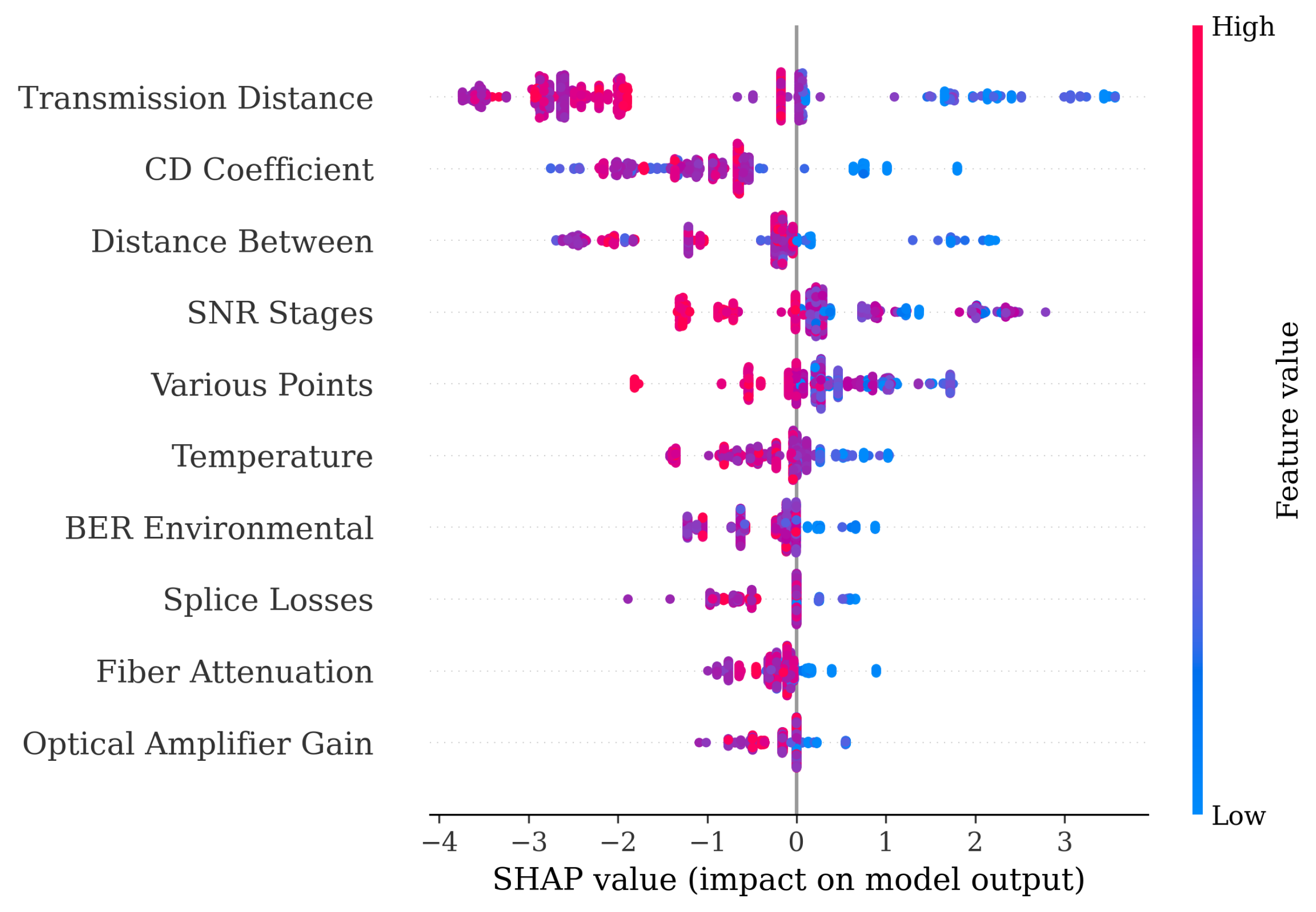
Figure 5 presents a bar chart with standard deviation error bars ranking the top-10 most important features by their mean absolute SHAP values, illustrating both the magnitude and variability of their contributions. Figure 6 is a bee swarm plot that shows the distribution of SHAP values for all samples and top features, providing insight into whether each feature generally increases or decreases the predicted QoT and how this effect varies across the dataset.

The analysis revealed that transmission distance is by far the most influential predictor, with a mean absolute SHAP value of 2.08 and the highest variability across samples, indicating that link length consistently drives significant changes in predicted QoT. The CD coefficient and distance between follow as the second and third most important features, reflecting the impact of chromatic dispersion and physical span length on signal quality. Parameters such as SNR stages, various points, and temperature also exhibit substantial contributions, highlighting the interplay between noise accumulation, network topology, and environmental conditions.

Beyond identifying the most influential features, SHAP analysis provides practical guidance for network operation and monitoring. Transmission distance, which consistently showed the highest SHAP values, indicates that long-haul links should be prioritized in quality monitoring systems, as even small changes in distance-related parameters can drive significant QoT degradation. Similarly, the chromatic dispersion (CD) coefficient and distance between spans emerged as dominant contributors, suggesting that dispersion management and span planning remain critical levers for maintaining network reliability. Environmental factors such as temperature and intermediate SNR stages also exhibited substantial SHAP contributions, highlighting the need to incorporate real-time environmental sensing and noise accumulation tracking in deployment.

From an operational perspective, these findings imply that monitoring systems should allocate more resources to features with consistently high SHAP influence while using less impactful features as supplementary indicators. Moreover, by observing shifts in SHAP importance across different augmentation settings, operators can detect when the decision process of a model becomes unstable, thus enabling proactive recalibration. In this way, the proposed interpretability analysis not only improves trust in ML-based QoT estimators but also offers actionable insights for field engineers in optical network maintenance.

5. Discussion

This work advances optical signal quality prediction by explicitly addressing robustness to noise, missing values, and distribution shifts—factors often overlooked in prior studies that focused mainly on clean laboratory data [5,6,10]. Our results confirm that models trained only on idealized datasets tend to overfit and perform poorly when exposed to realistic perturbations, consistent with observations in the broader ML literature [9]. By contrast, the proposed augmentation framework systematically introduces uncertainty into training, enabling more reliable generalization.

A key finding is that augmentation not only preserved clean-data accuracy but also markedly improved robustness under perturbations. While previous optical QoT studies rarely examined distribution drift, our controlled simulations of calibration mismatches and equipment aging provide a tractable approximation of real deployment conditions. Compared with earlier work, our approach offers the first systematic evidence that augmentation mitigates false positives under noisy scenarios, although some trade-off in precision remains.

Model-level comparisons also yield actionable insights. Tree-based ensembles consistently showed higher resilience than SVM and Naïve Bayes, confirming their suitability for deployment in noisy environments.

Finally, SHAP-based interpretability adds practical value. Beyond ranking features, our analysis highlights transmission distance and chromatic dispersion as dominant factors, suggesting long-haul links and dispersion-prone spans should receive closer monitoring. Environmental variables such as temperature also emerged as relevant, extending prior interpretability work by linking feature importance directly to operational guidelines.

6. Conclusions

6.1. Summary of Results

This study demonstrates that targeted data augmentations—Gaussian noise injection, structured label flipping, synthetic missingness with advanced imputation—can enhance model robustness against realistic perturbations in optical signal quality classification. Our results reveal that

• Label noise has the most severe impact, with performance degrading significantly beyond a 15–20% flip rate, particularly for Naïve Bayes and SVM.
• Feature noise up to moderate-to-high levels ($\sigma \le 0.75$) barely affects tree-based ensembles but impacts Naïve Bayes under extreme distortion.
• Missingness is well-tolerated when coupled with advanced imputation (MICE > KNN > Mean).
• The optimal augmentation setting (flip_rate = 0.10, noise_level = 0.50, missing_rate = 0.20) preserved clean test accuracy while substantially improving robustness under distribution shifts, raising accuracy from 0.863 to 0.950, precision from 0.384 to 0.632, F1 from 0.551 to 0.771, and ROC-AUC from 0.926 to 0.999 compared to training without augmentation.

These results demonstrate that modular augmentation pipelines not only mitigate sensitivity to perturbations but also deliver measurable performance gains, enabling practitioners to tune perturbation levels to field conditions and strengthen real-world generalization without sacrificing laboratory performance.

6.2. Future Work

Future research will focus on expanding the scope and realism of the experimental setup by incorporating operational data from diverse and dynamic network environments. This includes developing adaptive data augmentation strategies that automatically tune perturbation parameters based on observed data characteristics, rather than relying solely on fixed, expert-defined settings. Additionally, more sophisticated sensor drift models—capturing correlated impairments, nonlinear feature interactions, and temporal patterns such as seasonal or event-driven trends—will be explored to better replicate real-world degradation processes. These advancements will help improve the generalizability and robustness of QoT estimation models in practical deployments.