Author Contributions
Conceptualization, E.L. and X.H.; methodology, E.L.; software, J.Y.; validation, L.Z., A.W. and J.L.; formal analysis, E.L. and S.Y.; resources, W.S.; data curation, E.L. and Y.G.; writing—original draft preparation, E.L.; writing—review and editing, E.L. All authors have read and agreed to the published version of the manuscript.
Funding
This work was funded by the National Natural Science Foundation of China, Youth Science Foundation Program grant number 62205181, the Shandong University Education and Teaching Reform Research Program grant number 2022Y126, the National Foundation of China, Youth Science Foundation Program grant number 62205181, the Shandong Provincial Science and Technology Department, Excellent Youth Fund (Overseas) grant number 2023HWYQ-023, the Natural Science Foundation of Shandong Province, Youth Fund grant number ZR2022QF017, the Organization Department of Shandong Provincial Committee, Taishan Scholars grant number tsqn202211038, and Shandong University Education and the Teaching Reform Research Program grant number XYJG2023058.
Figure 1.
OCT B-scan images display the retinal layers of healthy human eyes alongside annotations of each specific retinal tissue layer. Figure (a) presents the original B-scan image of the retinal layers, while Figure (b) illustrates the annotated ground truth, identifying the eight distinct layers of the retina: the Nerve Fiber Layer (NFL), Ganglion Cell Layer + Inner Plexiform Layer (GCL + IPL), Inner Nuclear Layer (INL), Outer Plexiform Layer (OPL), Outer Nuclear Layer (ONL), External Limiting Membrane + Inner Segments (ELM + IS), Outer Segments (OS), and Retinal Pigment Epithelium (RPE). Annotations for regions classified as background are also included.
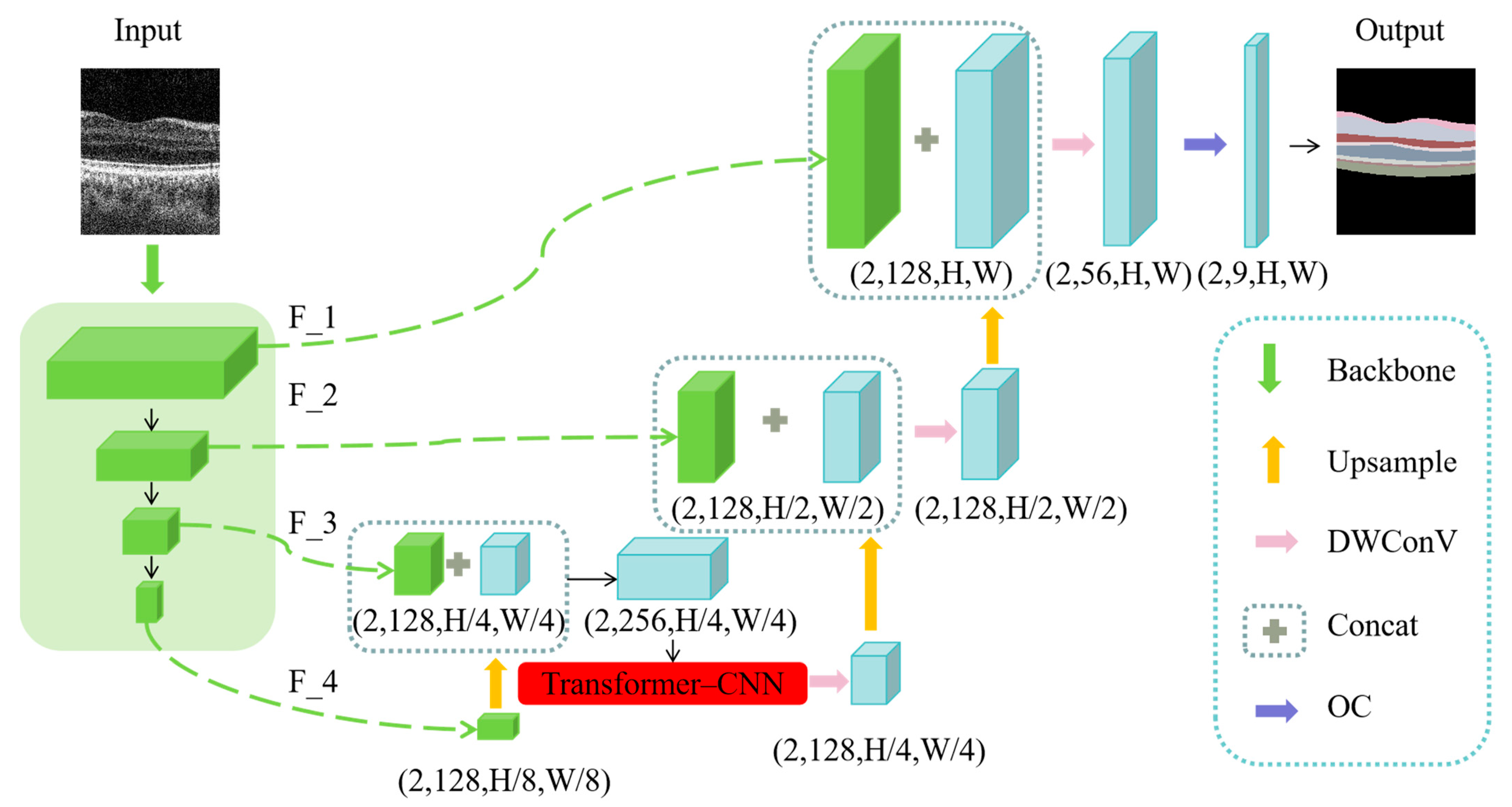
Figure 2.
Overall Network Architecture of MT_Net.
Figure 2.
Overall Network Architecture of MT_Net.
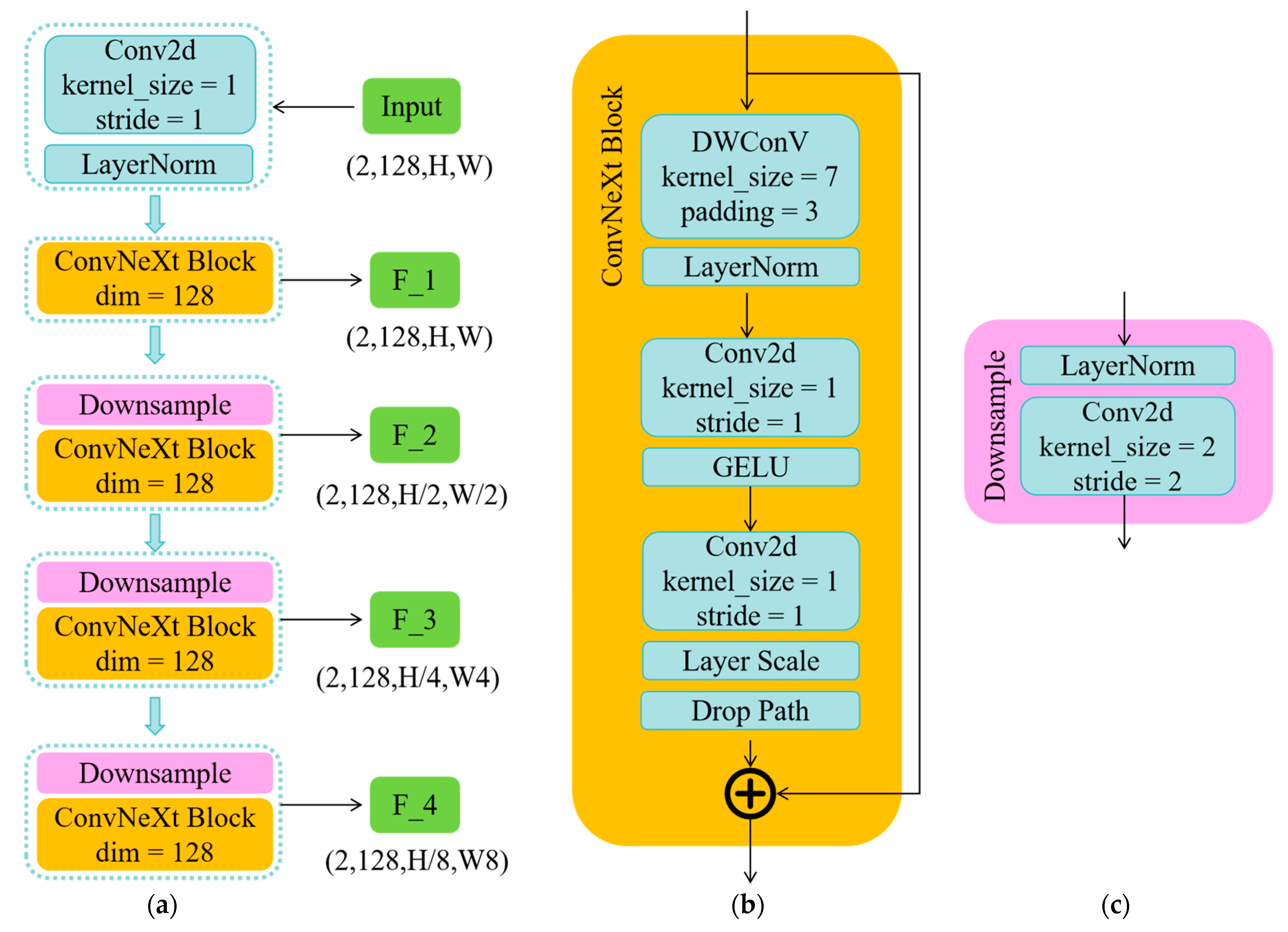
Figure 3.
The proposed method framework. Figure (a) depicts the overall framework of the ConvNeXt network, Figure (b) details the components of the ConvNeXt Block module, and Figure (c) illustrates the composition of the Downsample module.
Figure 3.
The proposed method framework. Figure (a) depicts the overall framework of the ConvNeXt network, Figure (b) details the components of the ConvNeXt Block module, and Figure (c) illustrates the composition of the Downsample module.
Figure 5.
System setup for vnOCT for human retinal imaging. BD: beam dump; PC: polarization controller. EFs: two edge filters.
Figure 5.
System setup for vnOCT for human retinal imaging. BD: beam dump; PC: polarization controller. EFs: two edge filters.
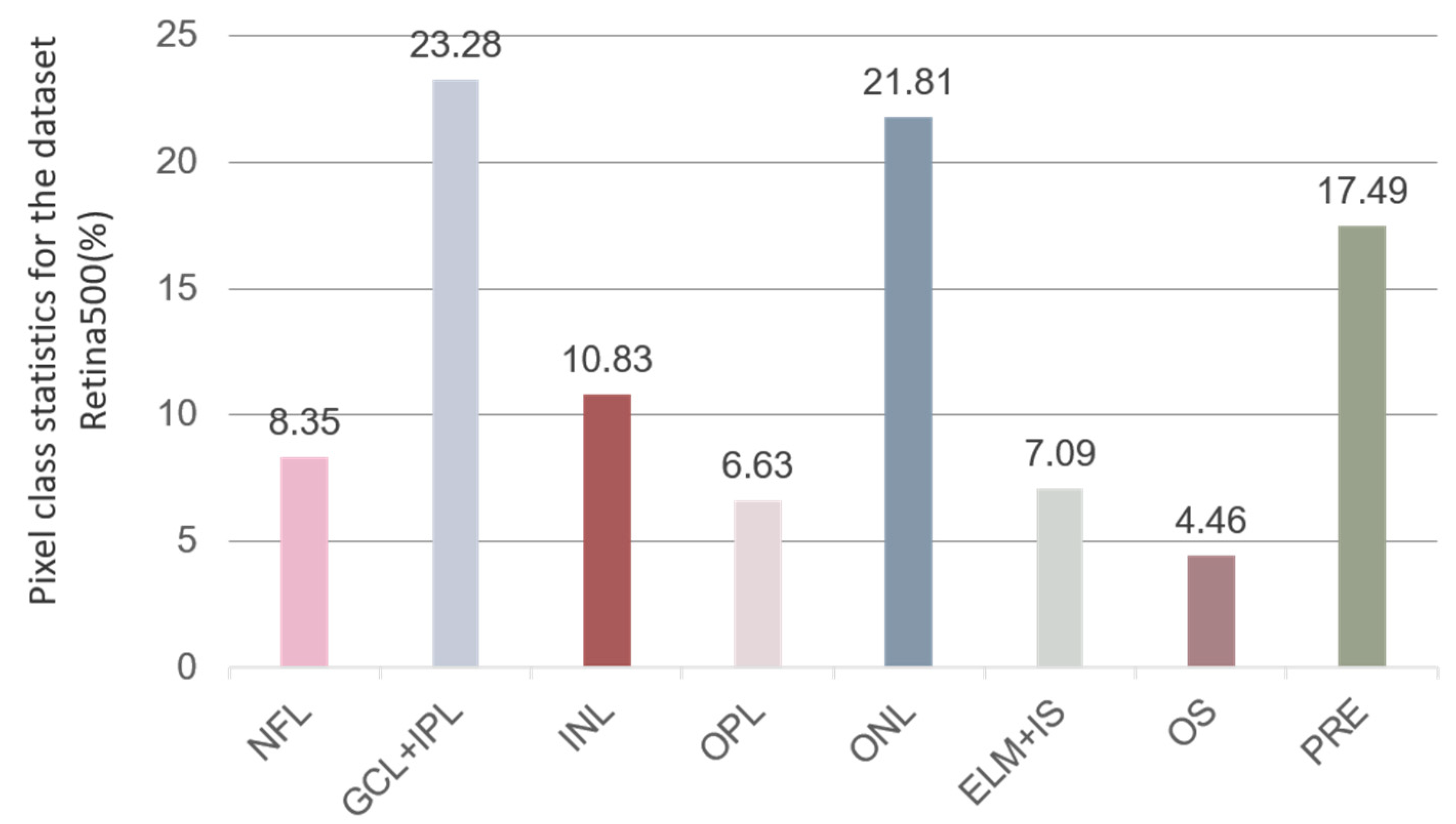
Figure 6.
The average percentage of pixels in each retinal layer in the Retina500 dataset among all retinal layers (excluding background).
Figure 6.
The average percentage of pixels in each retinal layer in the Retina500 dataset among all retinal layers (excluding background).
Figure 7.
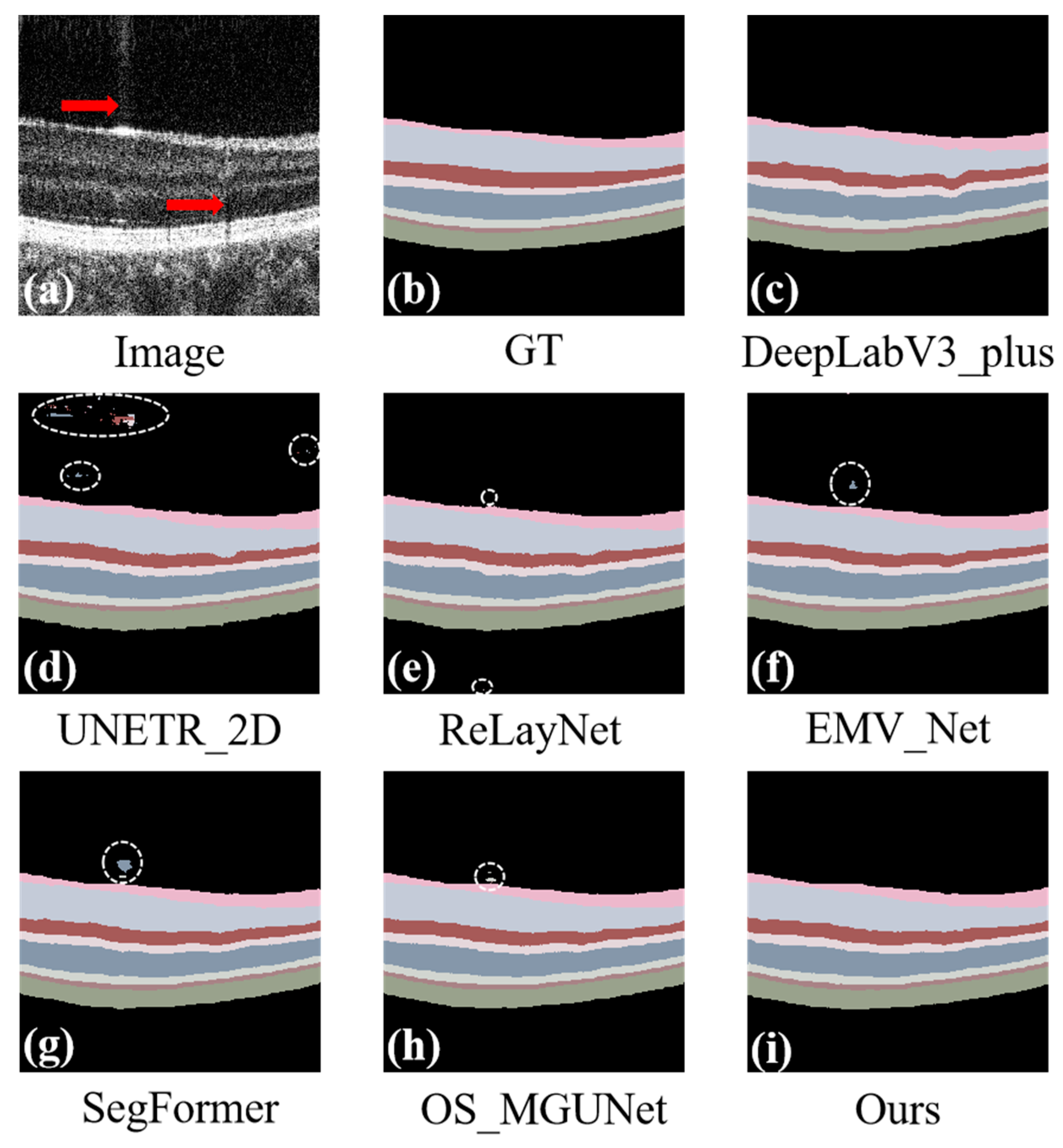
Predicted maps of retinal layer segmentation for randomized test images from the Retina500 dataset. Panel (a) displays the original image, and panel (b) shows the ground truth. The prediction maps are generated via various segmentation methods: DeepLab_v3+ in panel (c), UNETR_2D in panel (d), ReLayNet in panel (e), EMV_Net in panel (f), SegFormer in panel (g), OS_MGUNet in panel (h), and our proposed method in panel (i). Each panel demonstrates the effectiveness of the respective methods in segmenting the complex structures of the retinal layers.
Figure 8.
Segmentation effects of the model under the influence of noise and artifacts. Panel (a) displays the original image, and panel (b) shows the ground truth. The prediction maps are generated via various segmentation methods: DeepLab_v3+ in panel (c), UNETR_2D in panel (d), ReLayNet in panel (e), EMV_Net in panel (f), SegFormer in panel (g), OS_MGUNet in panel (h), and our proposed method in panel (i). Each panel demonstrates the effectiveness of the respective methods in segmenting the complex structures of the retinal layers.
Figure 9.
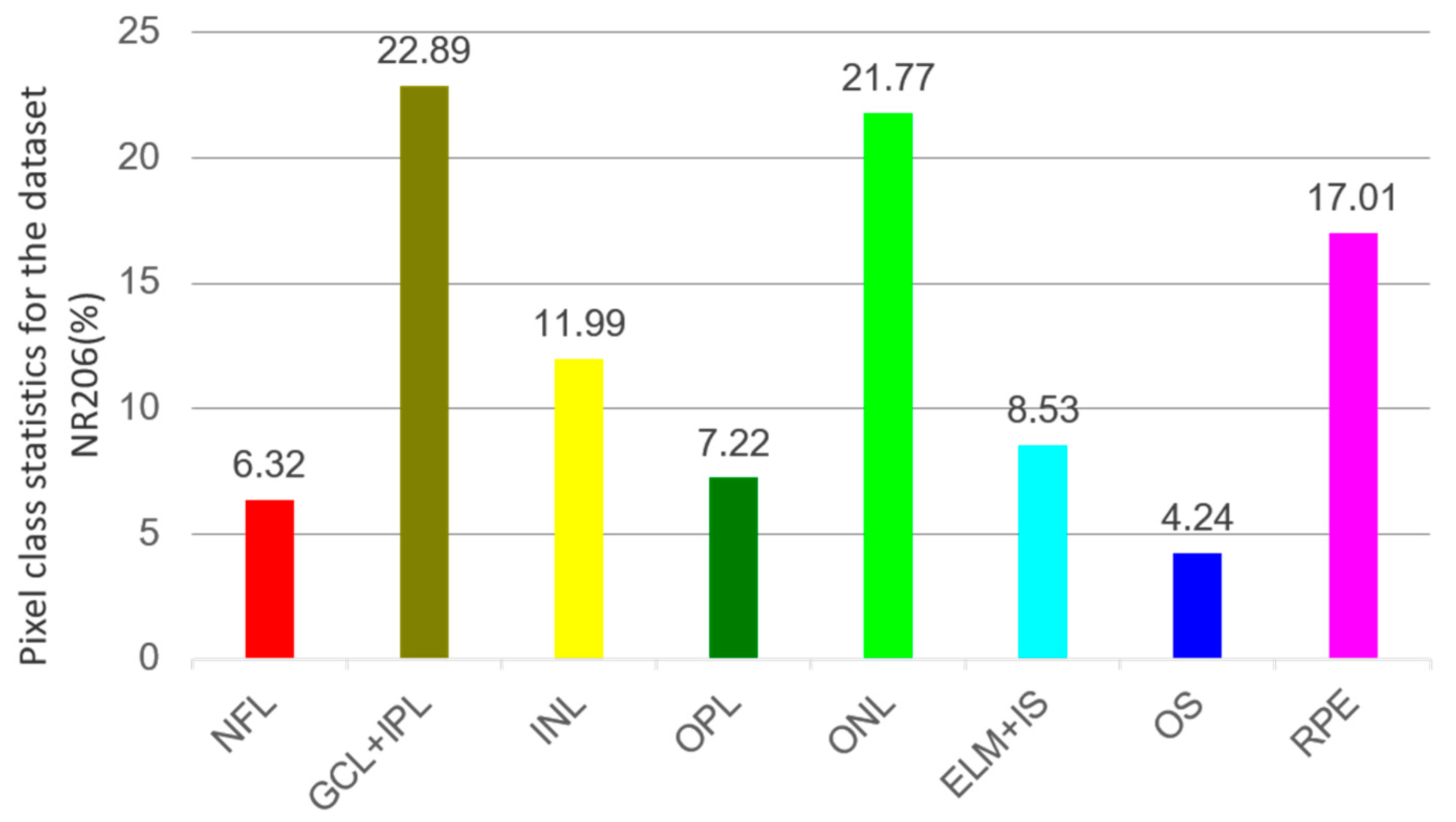
The average percentage of pixels in each retinal layer in the NR206 dataset among all retinal layers (excluding background).
Figure 9.
The average percentage of pixels in each retinal layer in the NR206 dataset among all retinal layers (excluding background).
Figure 10.
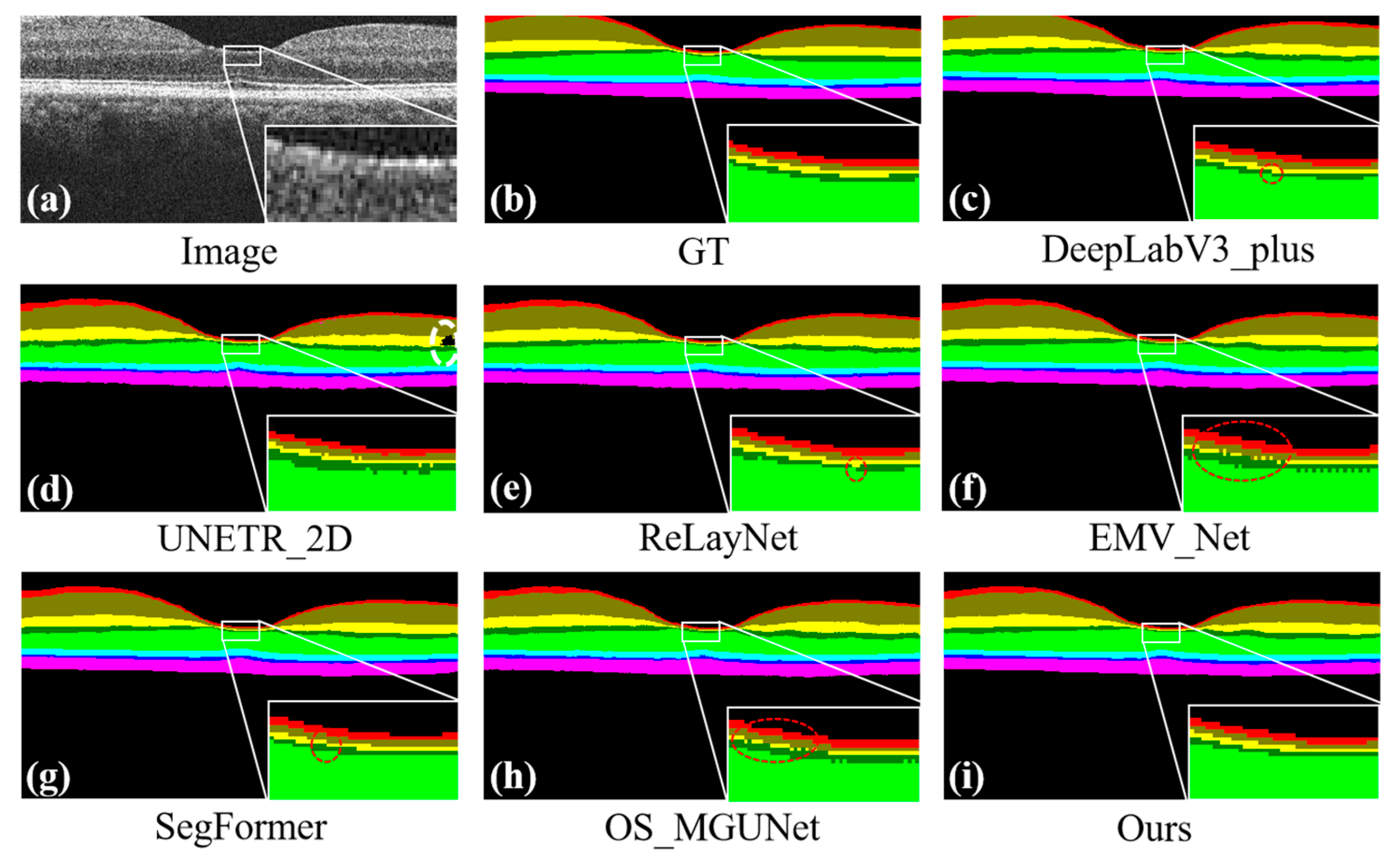
Predicted maps of retinal layer segmentation for randomized test images from the NR206 dataset. Panel (a) displays the original image, while panel (b) shows the ground truth. The subsequent panels illustrate the prediction maps generated by various segmentation methods: DeepLab_v3+ in panel (c), UNETR_2D in panel (d), ReLayNet in panel (e), EMV_Net in panel (f), SegFormer in panel (g), OS_MGUNet in panel (h), and our method in panel (i). Additionally, each panel includes a zoomed-in view to highlight the local details of the predictions, providing a closer look at the segmentation accuracy of each method.
Figure 11.
Ablation experiments performed on the Retina500 dataset, where (a) is the original image, (b) is the ground-truth, (c) is the prediction map without the Transformer module in our method, and (d) is the prediction map with the Transformer module in our method.
Figure 11.
Ablation experiments performed on the Retina500 dataset, where (a) is the original image, (b) is the ground-truth, (c) is the prediction map without the Transformer module in our method, and (d) is the prediction map with the Transformer module in our method.
Table 1.
Setup of datasets Retina500 and NR206.
Table 1.
Setup of datasets Retina500 and NR206.
| Dataset | Number | Train | Validation | Test |
|---|
| Retina500 | 500 | 400 | 50 | 50 |
| NR206 | 206 | 126 | 40 | 40 |
Table 2.
Quantitative comparison of evaluation indicators of various methods on the Retina500 dataset.
Table 2.
Quantitative comparison of evaluation indicators of various methods on the Retina500 dataset.
| Method | mIoU | Acc | mPA |
|---|
| DeepLab_v3+ [37] | 78.28 | 88.65 | 96.44 |
| UNETR_2D [38] | 78.62 | 89.49 | 96.17 |
| ReLayNet [14] | 80.14 | 90.22 | 96.58 |
| EMV_Net [35] | 80.24 | 89.99 | 96.65 |
| SegFormer [39] | 79.90 | 89.90 | 96.56 |
| OS_MGUNet [40] | 80.87 | 90.77 | 96.67 |
| MT_Net | 81.26 | 91.38 | 96.77 |
Table 3.
Dice score (%) of the segmentation results on the Retina500 dataset obtained by different methods.
Table 3.
Dice score (%) of the segmentation results on the Retina500 dataset obtained by different methods.
| Method | NFL | GCL + IPL | INL | OPL | ONL | ELM + IS | OS | RPE |
|---|
| DeepLab_v3+ [37] | 87.87 | 84.00 | 88.79 | 79.19 | 93.63 | 90.12 | 73.50 | 92.27 |
| UNETR_2D [38] | 86.54 | 92.71 | 87.50 | 79.13 | 93.33 | 91.62 | 79.15 | 92.21 |
| ReLayNet [14] | 88.46 | 94.00 | 89.54 | 81.59 | 93.58 | 90.46 | 90.13 | 92.35 |
| EMV_Net [35] | 88.49 | 93.75 | 88.92 | 82.34 | 94.29 | 91.56 | 78.36 | 92.61 |
| SegFormer [39] | 87.72 | 93.97 | 90.18 | 81.65 | 93.48 | 89.89 | 79.27 | 92.64 |
| OS_MGUNet [40] | 87.27 | 93.65 | 89.86 | 82.01 | 94.03 | 92.02 | 81.51 | 93.38 |
| MT_Net | 88.79 | 94.84 | 91.43 | 83.94 | 94.61 | 91.89 | 78.66 | 91.64 |
Table 4.
Quantitative comparison of evaluation indicators of various methods on the NR206 dataset.
Table 4.
Quantitative comparison of evaluation indicators of various methods on the NR206 dataset.
| Method | mIoU | Acc | mPA |
|---|
| DeepLab_v3+ [37] | 83.89 | 91.38 | 98.62 |
| UNETR_2D [38] | 83.07 | 90.29 | 98.50 |
| ReLayNet [14] | 83.95 | 90.80 | 98.64 |
| EMV_Net [35] | 83.59 | 91.25 | 98.56 |
| SegFormer [39] | 83.76 | 90.98 | 98.60 |
| OS_MGUNet [40] | 83.58 | 90.91 | 98.58 |
| MT_Net | 84.46 | 91.24 | 98.67 |
Table 5.
Dice score (%) of the segmentation results on the NR206 dataset obtained by different methods.
Table 5.
Dice score (%) of the segmentation results on the NR206 dataset obtained by different methods.
| Method | NFL | GCL + IPL | INL | OPL | ONL | ELM + IS | OS | RPE |
|---|
| DeepLab_v3+ [37] | 87.03 | 96.20 | 90.43 | 81.47 | 95.76 | 93.11 | 87.73 | 96.40 |
| UNETR_2D [38] | 87.05 | 95.60 | 88.82 | 79.37 | 95.42 | 93.00 | 88.29 | 96.37 |
| ReLayNet [14] | 87.82 | 96.33 | 90.57 | 80.31 | 95.78 | 93.35 | 87.61 | 96.44 |
| EMV_Net [35] | 86.98 | 96.09 | 90.31 | 81.38 | 95.81 | 92.85 | 87.45 | 95.85 |
| SegFormer [39] | 87.03 | 96.21 | 90.44 | 81.48 | 95.80 | 92.89 | 87.48 | 96.16 |
| OS_MGUNet [40] | 86.62 | 96.01 | 89.76 | 81.29 | 95.70 | 93.18 | 87.57 | 96.40 |
| MT_Net | 88.04 | 96.33 | 90.65 | 80.81 | 95.84 | 93.57 | 88.80 | 96.69 |
Table 6.
Inference time (s) statistics for various methods.
Table 6.
Inference time (s) statistics for various methods.
| Method | Inference Time |
|---|
| DeepLab_v3+ [37] | 1.87 |
| UNETR_2D [38] | 1.50 |
| ReLayNet [14] | 0.80 |
| EMV_Net [35] | 2.18 |
| SegFormer [39] | 1.16 |
| OS_MGUNet [40] | 1.36 |
| MT_Net | 3.16 |
Table 7.
Comparison of quantitative analysis on the Retina500 dataset through Transformer ablation experiments performed in our framework.
Table 7.
Comparison of quantitative analysis on the Retina500 dataset through Transformer ablation experiments performed in our framework.
| Method | Average_Dice | mIoU | Acc | mPA |
|---|
| No Transformer | 89.41 | 80.85 | 90.94 | 96.77 |
| MT_Net | 91.57 | 84.46 | 91.24 | 98.67 |
