Article

Real-Time Tracking of Photovoltaics by Differential Absorption Imaging in Optical Wireless Power Transmission

by
Kaoru Asaba
and
Tomoyuki Miyamoto
*
Laboratory for Future Interdisciplinary Research of Science and Technology (FIRST), Institute of Innovative Research (IIR), Tokyo Institute of Technology, R2-39, 4259 Nagatsuta, Midori-ku, Yokohama 226-8503, Japan
*
Author to whom correspondence should be addressed.
Photonics 2024, 11(6), 490; https://doi.org/10.3390/photonics11060490
Submission received: 12 April 2024 / Revised: 9 May 2024 / Accepted: 11 May 2024 / Published: 22 May 2024

Abstract

:
In the future, wireless power transmission is expected to cover power levels ranging from milliwatts to megawatts and over distances of a few meters to kilometers for both stationary and moving photovoltaic (PV) targets. Optical wireless power transmission (OWPT) is a promising solution for such multi-scale systems, which use the narrow beam divergence of light. To enhance the efficiency of power generation in PV targets, real-time detection of the target’s position and attitude is crucial for OWPT systems. The authors propose detecting the PV using differential absorption images as one such method. This paper investigates algorithms for tracking moving PV targets and evaluates their performance. The first algorithm combines thresholds with an autoregressive (AR) model, while the other two use estimation with Kalman filters. The comparison of tracking algorithms can be undertaken using a score function based on the position estimation error. The evaluation results indicate that the AR model combined with thresholds, on average, outperforms the other models. There was no significant difference between the approach involving use of a Kalman filter to estimate positions based on a uniform motion model and the approach involving use of a Kalman filter to estimate the AR model. The authors’ series of studies, from a former high-level requirement study to the current target tracking using differential absorption imaging, has verified a concept for one of the crucial processes in OWPT. These works form a step toward the practical implementation of OWPT systems.

1. Introduction

Wireless power transmission is expected to cover power levels ranging from milliwatts to several megawatts for stationary and moving targets, over transmission distances from a few meters to kilometers in future society [1]. Optical wireless power transmission (OWPT) is considered a promising candidate for such multi-scale systems, due to the narrow beam divergence of light [2,3,4,5]. To increase the power generation efficiency of photovoltaic (PV) targets, accurate beam alignment and shaping according to the target’s position and attitude are necessary [6]. Thus, real-time detection of the position and attitude of PV is crucial for OWPT systems. Although obtaining position information using satellites or indoor navigation systems is possible [7,8], the availability of such infrastructure for OWPT operations is not always guaranteed. Moreover, it is uncertain whether such systems meet the requirements of a specific OWPT system, and the estimation of the target’s attitude using such systems is limited. Therefore, research on position and attitude estimation specific to OWPT is necessary.
Previous research on the position and attitude estimation of targets in OWPT has been limited [9,10], and the authors faced challenges such as changes in background light due to weather conditions and diurnal variations, as well as misrecognition of surrounding objects. In OWPT, target detection should be minimally dependent on the background environment. One such method for detecting the target was proposed by the authors, and involved the use of differential absorption images of the target [11]. This method captures images of the target using the absorption wavelength ( λ O N ) and non-absorption wavelength ( λ O F F ) of the PV. If λ O N and λ O F F are close enough to each other, by generating the difference between these two wavelength images, the background will be canceled out and the PV image will be extracted. In a former study, the non-diffuse angle characteristics of the rear surface of the PV were investigated [12]. Then, position and attitude determination of stationary targets, using a combination of the differential absorption and stereo imagery, was reported [13]. It was found that a consistency condition, referred to as ‘integrity measure’, holds for the center coordinates of the target estimated from the left and the right images. It was also discovered that there exists a minimum exposure time for the integrity measure to hold, and that this depends on the attitude angle of the target. A physical model was constructed to determine this minimum exposure time under general conditions. The attitude angle estimation based on this model was reported in a previous paper [14], demonstrating that the method shows no degradation in accuracy near the normal, which is suitable for OWPT operations.
This paper discusses real-time position and attitude estimation for moving targets. For targets with non-diffuse reflection characteristics, the position estimation error increases when the target attitude deviates from normal to the light source. This can lead to outliers and data loss, which is particularly problematic in real-time consecutive position estimation. Thus, every PV tracking algorithm should include smoothing processes that appropriately handle outliers, interpolation processes that complement missing data, and position estimation and correction (if necessary) processes for the target. This paper compares the following three methods for the tracking algorithm and evaluates their performance.
  • A method utilizing an autoregressive (AR) model to correct the target position estimation when changes exceed the predetermined thresholds.
  • A uniform motion model estimated by a Kalman filter.
  • The AR model estimated by a Kalman filter.
An accuracy improvement is proposed for the estimation using the fact that the direction (azimuth angle) can be estimated with precision, as has been reported in a former paper [13]. It was found that some challenges must be addressed for the camera that will be used in real-time attitude estimation. These requirements must be considered when selecting or developing the appropriate hardware for the operational system. The authors conducted an analysis of the high-level requirements for OWPT beam alignment and shaping in a former study [6]. It is confirmed that this research and the former study are consistent.
Unlike traditional solar power generation, OWPT requires the detection of the PV from the transmitter, tracking it if necessary, and then irradiating the power beam. The authors’ series of studies validated a concept that is essential in OWPT and established a definite step towards the practical implementation of OWPT systems.
This paper is structured as follows: Section 2 provides a review of previous research papers focusing on positioning and attitude determination utilizing a combination of differential absorption and stereo imagery. In Section 3, the tracking of moving targets is discussed. This includes the optimization of the camera parameters used in experiments for successive position estimation, as well as presenting initial experimental results for position and attitude estimation. Section 4 explores three algorithms for tracking moving targets, accompanied by discussions on their evaluation metric. Section 5 discusses algorithmic improvements and introduces the error model of the metric. Section 6 concludes the paper with a comparative analysis of a system-level misalignment requirement proposed in a former study. In Appendix A, data are added to support the discussion in Section 5.

2. Review of Positioning and Attitude Determination of PV by Differential Absorption Imaging

The section below discusses the application of the principle of position determination using differential absorption and stereo imaging, along with the introduction of an integrity measure as a consistency condition in position determination. The information presented here is based on former research papers [12,13,14].
In this method, a total of four infrared image sensors are required. These sensors correspond to the left and the right images of λ O N and of λ O F F 
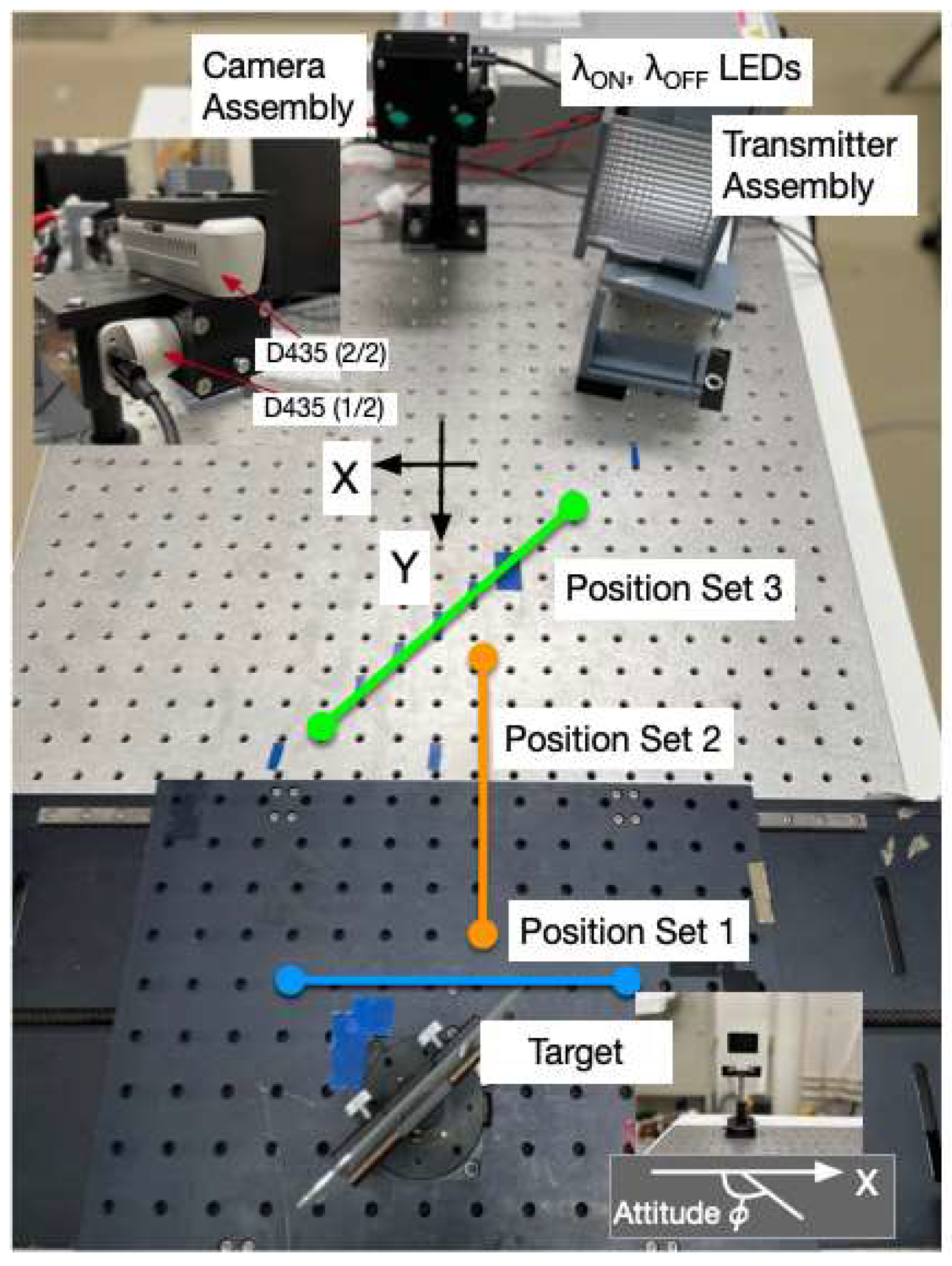
, respectively. The left and the right differential images are generated and binarized. The center coordinates of the target are estimated from these images, and the position of the target is then determined from their parallax. To evaluate the accuracy of the target position determination, experiments were conducted by varying the position and attitude of the target. The layout of the experimental setup is shown in Figure 1. Two Intel D435TM depth cameras were used in the experiments. These have two image sensors per unit [15] and were assembled as per the camera assembly shown in the figure. Although these cameras can generate depth information, this feature was not utilized in the experiments in this paper and the former papers. Instead, output from the camera assembly was processed by independent software to generate the differential absorption images and target’s position. The software was developed in PythonTM [16] for camera control, real-time position determination, and data output. Then, the position data processing to estimate the target’s tracked position was implemented in MathematicaTM [17]. The Python program ran on a Dell OptiPlex 7040 PC running Windows 10 OS, including an Intel(R) CoreTM i7-6700 CPU with a speed of 3.41 GHz and 16 GB RAM.
The optical bench used in the experiment has 23 (horizontal) × 31 (vertical) threaded holes arranged with a pitch of 25.4 mm. They are considered as lattice points in the 2D coordinate system 11 x   11 , 3 y   27 . In this paper, X and Y coordinates are represented using these coordinates. In the experiment, the target was placed at positions selected from Figure 1 and position sets 1, 2, and 3.
Position set 1: (−3, 27), (−2, 27), (−1, 27), (0, 27), (1, 27), (2, 27), (3, 27)
Position set 2: (0, 27), (0, 26), (0, 25), (0, 23), (0, 19)
Position set 3: (−4, 11), (−2, 13), (−1, 14), (0, 15), (1, 16), (2, 17), (4, 19)
It should be noted that the target in the experiment was not necessarily moving exactly along these position sets. The true track is displayed in each plot figure. Table 1 summarizes the experiment parameters, and specific details are outlined in a former paper [13].
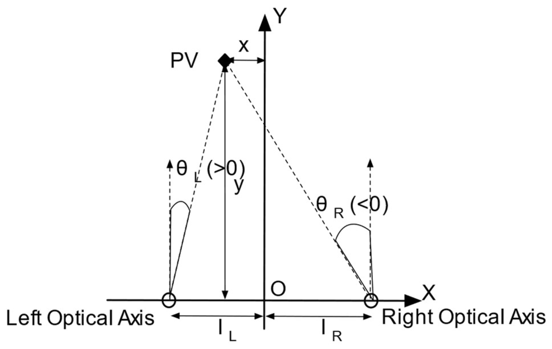
The camera assembly was positioned at the coordinate origin 0,0 . There are two optical axes of the left and right image sensors shown in Figure 2 (left and Right optical axis). These define the XY plane and are aligned parallel along the Y-axis.
The output image size of the sensors was set to 640 × 480 pixels. The origin 0 ,   0 of the pixel coordinate system for the image sensors is defined at the lower-left corner. The pixel coordinates ξ ,   η for both the left and the right image sensors are defined as 0 ξ 639 and 0 η 479 , respectively. Let the left and the right pixel coordinates of the target be ξ L , η L and ξ R ,   η R , respectively. The target position x ,   y in the 2D plane can then be determined from Figure 2, as follows:
x = ξ L 320 l L + l R ξ L ξ R l L
y = l L + l R θ ξ L ξ R
where l L and l R are known dimensions, with values of 17.5 mm and 32.5 mm, respectively, according to the D435 datasheet. θ is a constant that depends on the experiment system, which has been described in a former paper [13].
θ = 2.6   m r a d / p x
The target’s center coordinates, (ξL, ηL) and (ξR, ηR), should correspond with the same point. From the obtained pixel coordinates of the target, the consistency conditions (integrity measure) given by Equations (4) and (5) holds.
C1: ξLξR > 0
C2: ηLηR = 0
It is important to note that the integrity measure behaves randomly when the exposure time of the image sensor is short. However, it rapidly converges for values above a certain threshold. This minimum exposure time can be used to estimate the attitude angle of the target. A physical model was established in order to determine the minimum exposure time required for any given target position [14]. Leveraging this physical model and the measurement of the minimum exposure time allows the attitude angles of the target to be estimated.

3. Experiments of Real-Time Successive Positioning and Attitude Determination of the PV

3.1. Experiments Configuration and Tuning of Camera Parameters

The experiments described in this paper utilized two D435 cameras designated for receiving λ O N (camera 1) and λ O F F (camera 2). Before conducting successive position estimation experiments, it was necessary to determine the maximum data rates available using these two cameras, evaluate the latency between them, and estimate the time required for position estimation. The data rate and latency depend intrinsically on D435, while the time for position estimation depends on the PC and the operating system (OS) used in the experiments. Furthermore, appropriate parameters must be set in advance. There are two methods for synchronizing the two D435 cameras: hardware synchronization and software synchronization [18]. In this experiment, software synchronization was employed. Data acquisition from camera 1 and camera 2 was sequenced as follows and is depicted in Figure 3.
  • Initiating data stream for camera 1:
The data stream for camera 1 was commenced by issuing a command. Upon the arrival of data in the buffer, a timestamp (T1) was obtained.
2.
Wait command for camera 1:
Following the acquisition of T1, a wait command (wait1) was executed.
3.
Data acquisition for camera 2:
For camera 2, two options were considered for issuing commands. One option was using the ‘poll’ command, which enabled the obtaining of data from camera 2’s buffer along with its timestamp (T2) at T1+wait1. The other option was to use the ‘wait’ command to retrieve the subsequent data and timestamp (T’2) from camera 2’s data stream [19,20].
Using the measurement W P T 2 T 1 , taken by using the poll command for camera 2, and W W T 2 T 1 , by using the wait command, the camera’s internal frame rate (FR) for its exposure time (ExpTime) was estimated according to the model in Equation (6).
W W W P = 100 m s e c + E x p T i m e 1 / F R + 1 1 F R
The bracket ( [   ] ) in Equation (6) represents the integer part. The fitting results for FR as an integer based on the measured W W W P are presented in Figure 4.
In the experiments of static target position estimation in former papers, exposure times of 100 or 200 ms were significant. Given that the frame rate is 2 Hz when the exposure time is 200 ms in Figure 4 and considering the data processing time in PC and OS, a wait time (wait2) in Figure 3 was set as 1 s. In addition to this, the decision was made to utilize the combination of camera 1 with a wait command and camera 2 with a poll command over the wait/wait configuration, as the former was anticipated to result in a smaller latency between camera 1 and camera 2. The latency between camera 1 and camera 2 was measured by varying wait1 in Figure 3, and the results are presented in Figure 5.
In Figure 5a, the latency for 50 successive data is depicted when wait1 is set to 18 ms and exposure time (exp time) is 200 ms. In this case, the latency takes two values: +100 ms and −160 ms. Figure 5b plots the maximum minus (−) the minimum latency normalized by the camera’s exposure time (exp time). The clustering of data around 1 on the vertical axis indicates that the latency fluctuates over the entire width corresponding to exp time. While the latency does not exhibit strong dependency on wait1, wait1 was set to 18 ms for exp time = 200 ms and 12 ms for 100 ms in this paper. The deviation from 1 on the vertical axis of Figure 5b for shorter exp time can be attributed to the time taken to estimate the position.
Figure 6a shows the time sequence for 50 consecutive position estimations, revealing that it took approximately 60 s for this process. It should be noted that about 8 s were allocated for the initial set camera profile and start stream and the final stop stream processes. On the other hand, a large portion of time spent on capture data and position estimation was attributed to wait2 in Figure 6. Figure 6b displays the net time for capture data and position estimation, obtained by subtracting wait2 (=1 s) from the total time. The processing time required for position determination was within the range of 30 to 40 ms. It is worth noting that this value depends on the performance of the PC and OS used in the experiments.

3.2. Real-Time Positioning of the PV

The initial experiment of 50 consecutive position estimations was carried out using the setup depicted in Figure 7a. The target mounted on the rotation stage was fixed on the linear stage and manually translated. During experiments involving varying the attitude angles, deviation of the attitude angle from around 90 degrees caused data to fail to meet the integrity measure, and consequently led to a higher rate of data loss. The results for position set 1 (ϕ = 85 degrees) are shown in Figure 7b. Similar observations were made for position sets 2 and 3. These issues are addressed in Section 4 and Section 5.

3.3. Successive Attitude Determination of the PV

Like successive position estimation, it is feasible to estimate attitude angles in real time using the method described in Section 2. Figure 8 illustrates the outcomes of the attitude angle estimation, while fixing the target at (0, 27) and varying its attitude from 40 to 120 degrees. To estimate the attitude using the integrity measure, it is necessary to search for the minimum exposure time at which it converges. During the experiment, the current minimum value was searched around the previous value while varying the attitude angles.
The estimation error was minimized in the neighborhood of the normal direction. Furthermore, the time required for estimation depends on the number of searches conducted for the minimum exposure time and was typically about 10 to 15 s. This duration is explained by the set camera profile and start stream and stop stream functions, which are necessary for each search iteration, as illustrated in Figure 6a.
In summary of Section 3, some challenges pertaining to successive position estimation and real-time attitude angle estimation are identified. One such challenge is the latency between camera 1 and camera 2, as seen in Figure 5. However, since the velocity of the target is roughly 0.1 unit/s, the latency between the two cameras is not an issue in the current experiments. Furthermore, this latency can be minimized by synchronizing the two cameras using hardware. Another challenge is the time required for the set camera profile and start stream and stop stream functions, shown in Figure 6a. Although this time is not negligible, it is not an inherent issue with the proposed method in this paper. This challenge can be effectively addressed by designing the camera system with an awareness of this aspect, thereby optimizing the overall performance of the system. Using a high-speed PC and compiled application software, the time for positioning would reduce from 30~50 ms to 20 ms or less. If the time for the start frame can be reduced from 2 s to 50 ms and the time for the stop frame from 6 s to 50 ms, the total time, including positioning and start/stop stream, can be reduced to less than 120 ms. Because, as we find from Figure 8b, there needs to be twice the search iteration to find the minimum exposure time, this makes the attitude estimation 4 Hz (=1/(2 × 120 ms)). Suppose that attitude angular velocity of the target is 90 deg/10 s, then, attitude would be measured with a 2.25-degree error. In comparison with that shown Figure 8a, this would be acceptable.

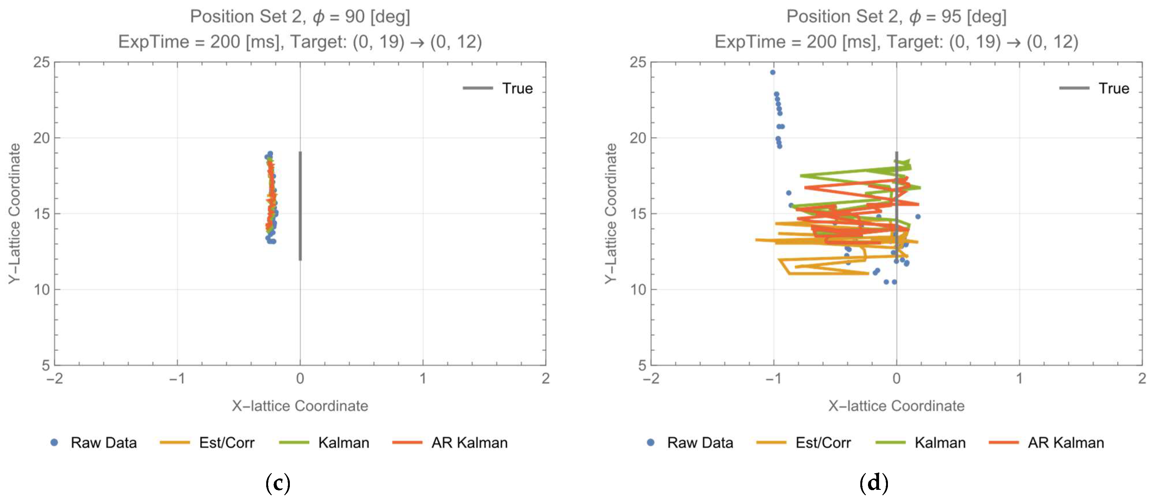
4. Tracking of the PV
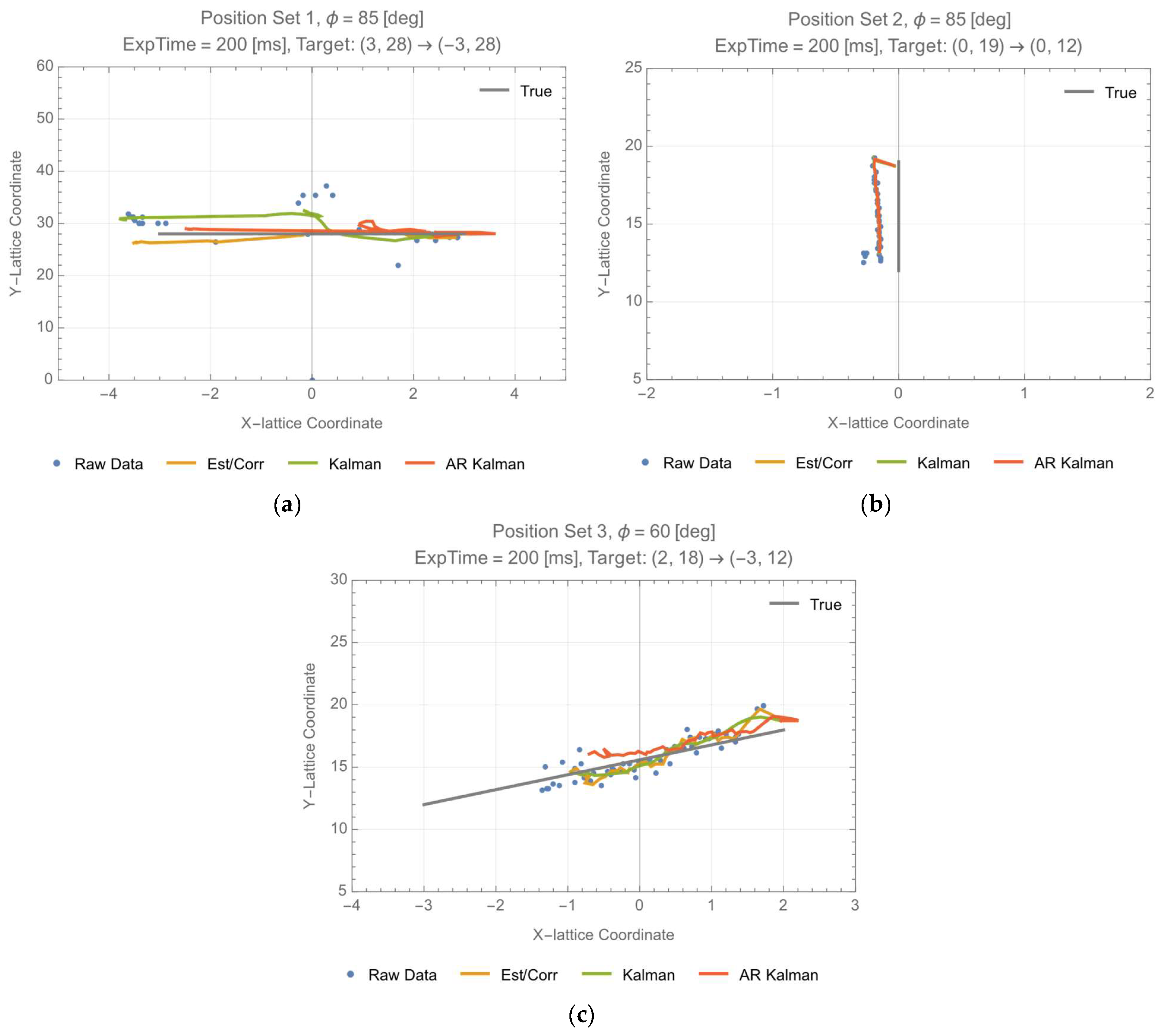
In Figure 7b, there are outliers near the position estimation at x = 0 , and there is data loss around x = 1 . Data loss can happen when the attitude angle ϕ deviates from the normal to the transmitter, even when the received light is excessively intense near the normal direction. Since Figure 7b is for data with angles close to the normal direction (ϕ = 85 deg), outliers and data loss were likely caused by excessively intense light.
To address the issue of outliers and missing data, it is necessary to appropriately interpolate the raw data, smooth it, and correct outliers. In this section, three algorithms are discussed for this purpose. To assess the algorithms, a score function is defined based on the true values of the target positions.

4.1. Tracking Algorithms

Three tracking algorithms are presented. The first employs a combination of thresholds and an autoregressive (AR) model. It is a supervised anomaly rejection algorithm and requires training before operation. On the other hand, the other two algorithms use Kalman filters for estimation and do not require any training.

4.1.1. AR Model with Threshold (Estimator/Corrector)

The raw data from successive position estimation can be interpreted as time-series data. Analyzing such data using an autoregressive model, including outlier handling, is widely used in various fields [21,22].
  • Raw data (measurement) processing (the primary smoothing)
Let x n and x n + 1 be two successive raw data (measurements). If the change from x n to x n + 1 does not exceed a predefined threshold, neither smoothing nor interpolation is performed. If the change from x n to x n + 1 exceeds a predefined threshold T or x n + 1 is missing, primary smoothing and interpolation of missing data for the (n + 1)-th position data x n + 1 are executed as per Equation (7).
x n + 1 = x n + 1 , x n + 1 x n T 1 2 2 x n x n 1 + 2 x n 2 + x n 3 , x n + 1   i s   m i s s i n g   o r     x n + 1 x n > T
2.
Estimator (the secondary smoothing and the primary estimate)
After the primary smoothing, the secondary smoothing is carried out using a Butterworth low-pass filter [23]. The cutoff frequency of the filter is set to ω c = 0.1 rad/s, and its order is N = 8. The outcome of this process is referred to as the primary estimate, which is denoted as x n .
3.
Corrector (the secondary estimate)
The process applies the same procedure to x n as per Equation (7), then results in the secondary estimates (tracker output) x n . The thresholds in this case are denoted as T .
The above three processes are applied to the X coordinate and the Y coordinate estimations. The specified thresholds for each are T x ,   T y = 2 ,   2.3 and T x ,   T y = 1 ,   2 . Before tracking, the initial data for the AR model and the low-pass filter are needed. The median of 50 consecutive position determinations for the stationary target was used for this purpose, and it was then duplicated as necessary (four times for the AR model and eight times for the low-pass filter). This algorithm requires acquiring data before its operation and to optimize both T x , T y and T x , T y beforehand.

4.1.2. Uniform Motion Model Estimated by Kalman Filter (Kalman)

Algorithm in Section 4.1.1, the estimator/corrector, is a supervised model that requires threshold optimization through training. On the other hand, in Section 4.1.2 and Section 4.1.3, models that do not require any training are explored.
Assuming no external force on the target, the steady state Kalman filter [24] is used to estimate the position and the velocity of the n-th data point. Let measurement X n = x n ,   x ˙ n T , and the raw data for x ˙ n be given by x ˙ n = x n x n 1 Δ t . The prediction for the n-th data using the data up to (n − 1)-th estimation is denoted as X n , and the estimation for the n-th data using the data up to n-th measurement and the n-th prediction is denoted as X n . The corresponding state equation is given by Equation (8a), Equation (8b), Equation (8c), and the observation equation is by Equation (9a) and Equation (9b).
X n = F X n 1 + G w
F = 1 t 0 1
G w 2 G T = 0 0 0 w 2
x n = H X n + R
H = 1 ,   0
In this experiment, the fact that the data rate is 1 Hz implies t = 1 . Let N μ ,   σ a Gaussian distribution with mean μ and standard deviation σ . The system noise w is assumed to be w ~ N 0 ,   0.05 . Similarly, the measurement noise is assumed to follow R ~ N 0 , Σ , where Σ represents the standard deviation during initial value determination. The estimation X n can be obtained using the prediction X n , the measurement x n and the Kalman gain K as follows:
X n = X n + K x n H X n
  • Raw data processing
In case of missing raw data, the missing values are interpolated using Equation (11), as follows:
X r a w , n = F X r a w , n 1
2.
Smoothing
The interpolated raw data X r a w ,   n are input to the same Butterworth low-pass filter as in Section 4.2.1. The resulting values are denoted as X n .
3.
Position estimation (tracker output)
The n-th prediction X n is obtained from Equation (8a) using the (n − 1)-th estimation X n 1 . Along with x n = H X n , the n-th estimation X n is calculated using Equation (10). The final tracker output is x n = H X n . This process is applied to both the X-coordinate and the Y-coordinate estimations. The initial values generation process is the same as in Section 4.1.1.

4.1.3. AR Model Estimated by Kalman Filter (AR Kalman)

Additionally, estimation using a Kalman filter for an AR model is widely employed in the analysis of time-series data [25,26,27]. In this algorithm, the AR model in Equation (7) is estimated using a Kalman filter. Equation (8b), Equation (8c), Equation (9b) are replaced by Equation (12c), Equation (12d), Equation (12e).
X n = x n ,   x n 1 ,   x n 2 ,   x n 3 T
X n = F X n 1 + G w
F = 1 1 2 1 1 2 1 0 0 0 0 1 0 0 0 0 1 0
G w 2 G T = 3 · w 2 0 0 0 0 w 2 0 0 0 0 w 2 0 0 0 0 w 2
H = 1,0 , 0,0
Equation (11) is replaced by a similar equation as Equation (12b). The estimation procedure used to obtain the tracker output is x n = H X n , and the initialization method is the same as in Section 4.1.1.

4.2. Assessment of the Three Algorithms

4.2.1. Score Function and Estimation of True Position

The algorithms from Section 4.1.1, Section 4.1.2 and Section 4.1.3 enable tracking of the target. An excerpt from the tracking results is shown in Figure 9. The procedure to generate the tracking plots in this paper is as follows.
  • The Python program outputs position data in real time and each measurement (position determination) is successively stored in a list (list A).
  • The Mathematica program takes measurement data from list A and estimates its tracked position one by one using the algorithms. Then, each estimation is successively stored in a list (list B).
  • The tracking plots are generated from list B.
It should be noted that, except for the plot generation process using Mathematica, the rest is conducted on an essentially real-time basis. When comparing these algorithms under the same target distance, etc., because the amount of computation is not so different among the three algorithms, the difference appears in tracking errors.
To assess the performance of the algorithms, a score function is defined. It quantifies the tracked results.
S c o r e = 100 1 + e
e = 1 N i = 1 N e i
where e i denotes a position error associated with each tracked target data, and e represents the average over N (=50) data of the tracking process. Each e i is defined as follows:
e i = x i x t , i 2 + y i y t , i 2
where x i , y i are the i-th estimates obtained by the algorithms. On the other hand, x t , i , y t , i are the true values of the target, which are generally determined by measuring the target position using an independent device from the experimental setup in Figure 1. However, this paper proposes a simpler method to estimate them.
The score utilizing e i defined by Equation (14) is referred to as the true position (TP)-based score in this paper. A former study has shown that estimating the direction angle ψ , defined by t a n ψ = x y , is more accurate compared with the position estimation x ,   y [13]. The direction error Δ ψ , due to position estimation errors Δ x and Δ y , is obtained by Equation (15), where ξ L R is the horizontal coordinate in the left (right) image sensor of the target, and Δ ξ L R represents its error.
Δ ψ = y Δ x x Δ y x 2 + y 2 = y 2 x 2 + y 2 ξ L Δ ξ R + ξ R Δ ξ L ξ L + ξ R Δ θ
Assuming ξ L and ξ R are quantities of the same order, and assuming the same for Δ ξ L and Δ ξ R , the evaluation of Δ ψ is approximated as Δ ψ ~ Δ θ Δ ξ R L = 2.6   m r a d 0.15   d e g × Δ ξ R L p x . By re-evaluating the accuracy of the direction angle estimation from the data included in a former paper [13], 
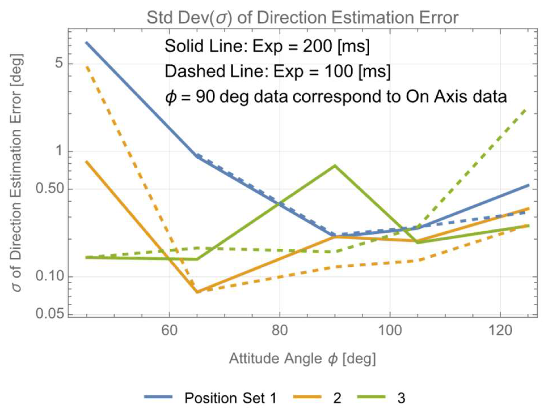
Figure 10 is obtained. The actual experimental data included a constant offset that varied from day to day, and this constant offset is due to errors in the daily setup of the experimental apparatus. In Figure 10, the accuracy of the direction angle estimation is evaluated by the standard deviation across each position set, excluding this offset.
From Figure 10, the accuracy of the direction angle ψ estimation varies with the target’s attitude angle ϕ, and ψ 
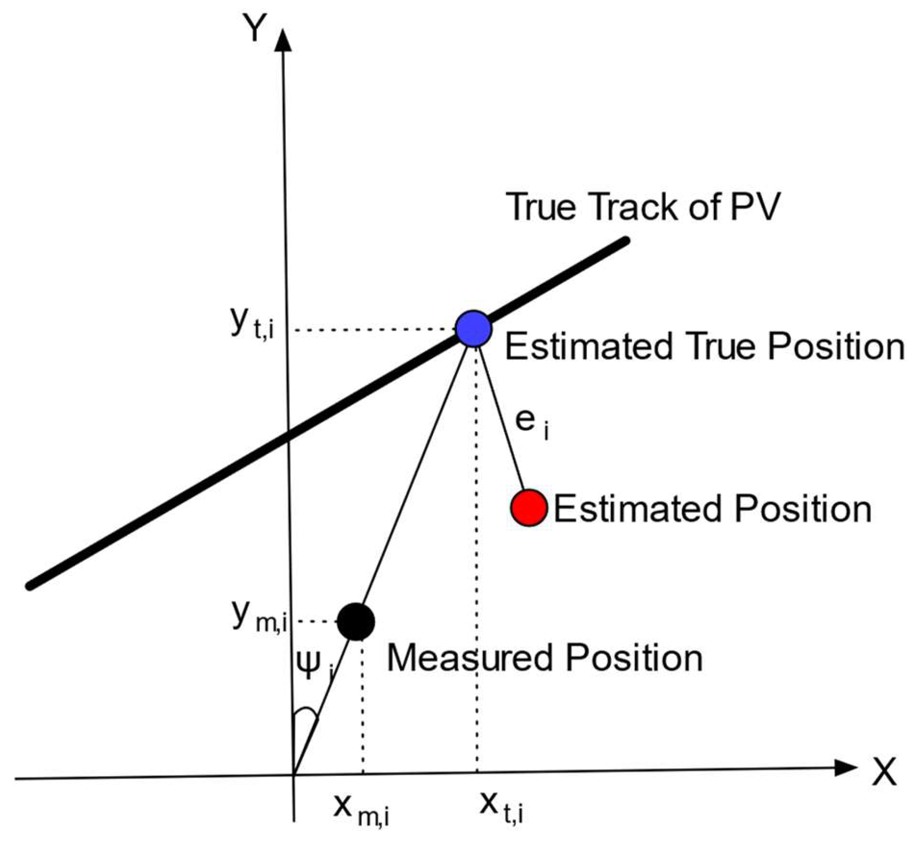
can be estimated with an accuracy of approximately 0.15 degrees when the target is close to the normal direction. From Equation (15), this corresponds to about 1 pixel error in the pixel coordinate system, which can be regarded as the measurement limit. Then, the true position can be estimated by the intersection of the true track of the target, which is known in the experiments and the line x i = y i t a n ψ i as depicted in Figure 11. e i can be calculated from Equation (14) as the distance between the estimated position by the algorithm and the estimated true position.

4.2.2. Assessment of the Three Algorithms

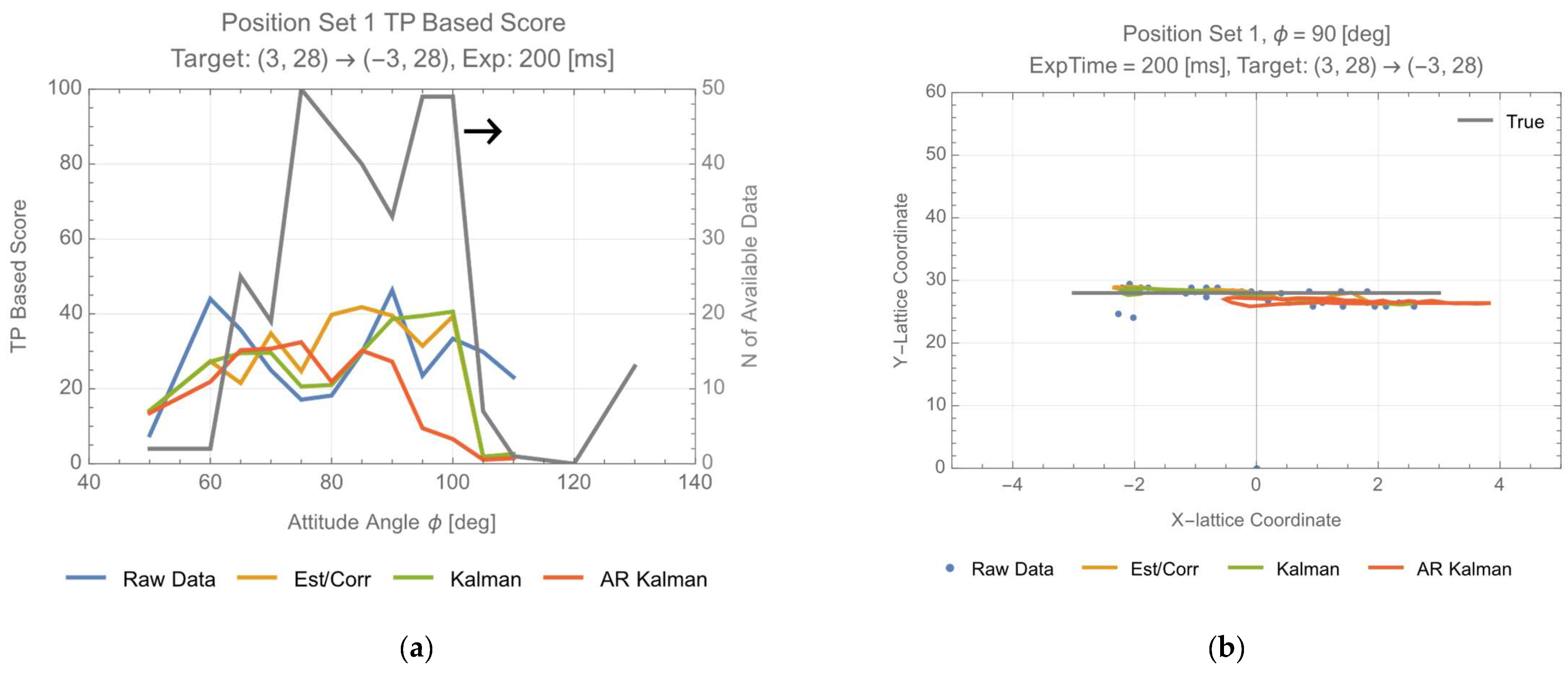
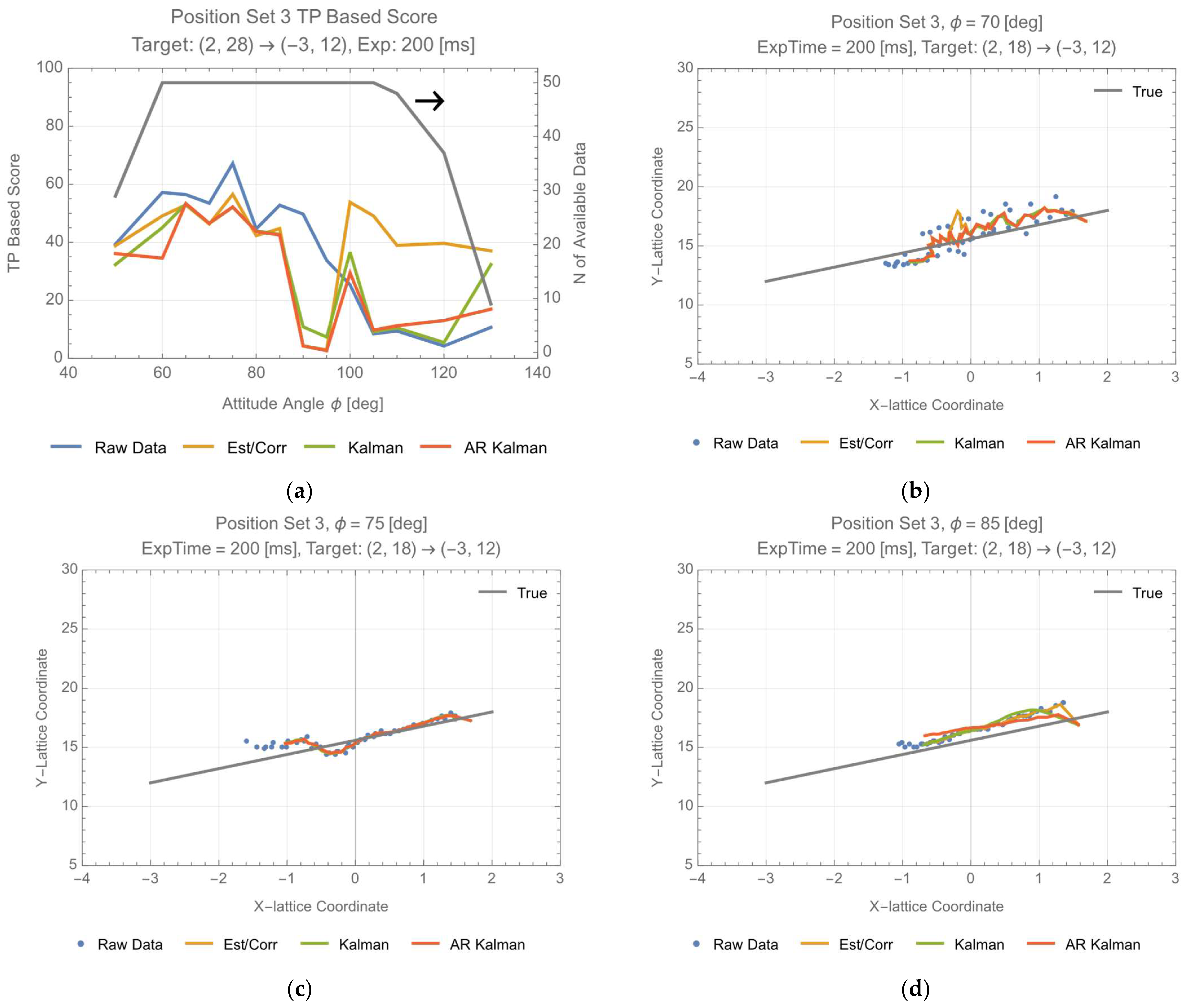
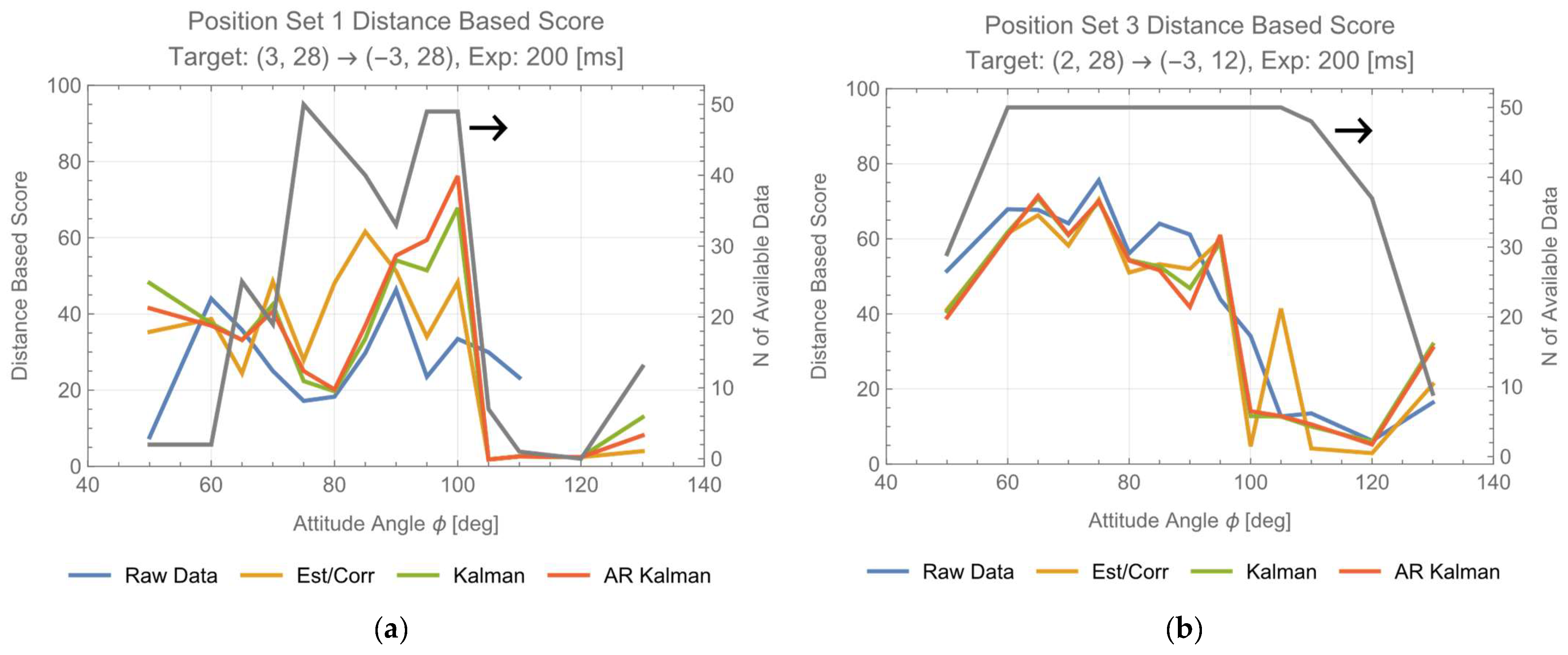
The results of the TP-based score are displayed in Figure 12 (position set 1) and 
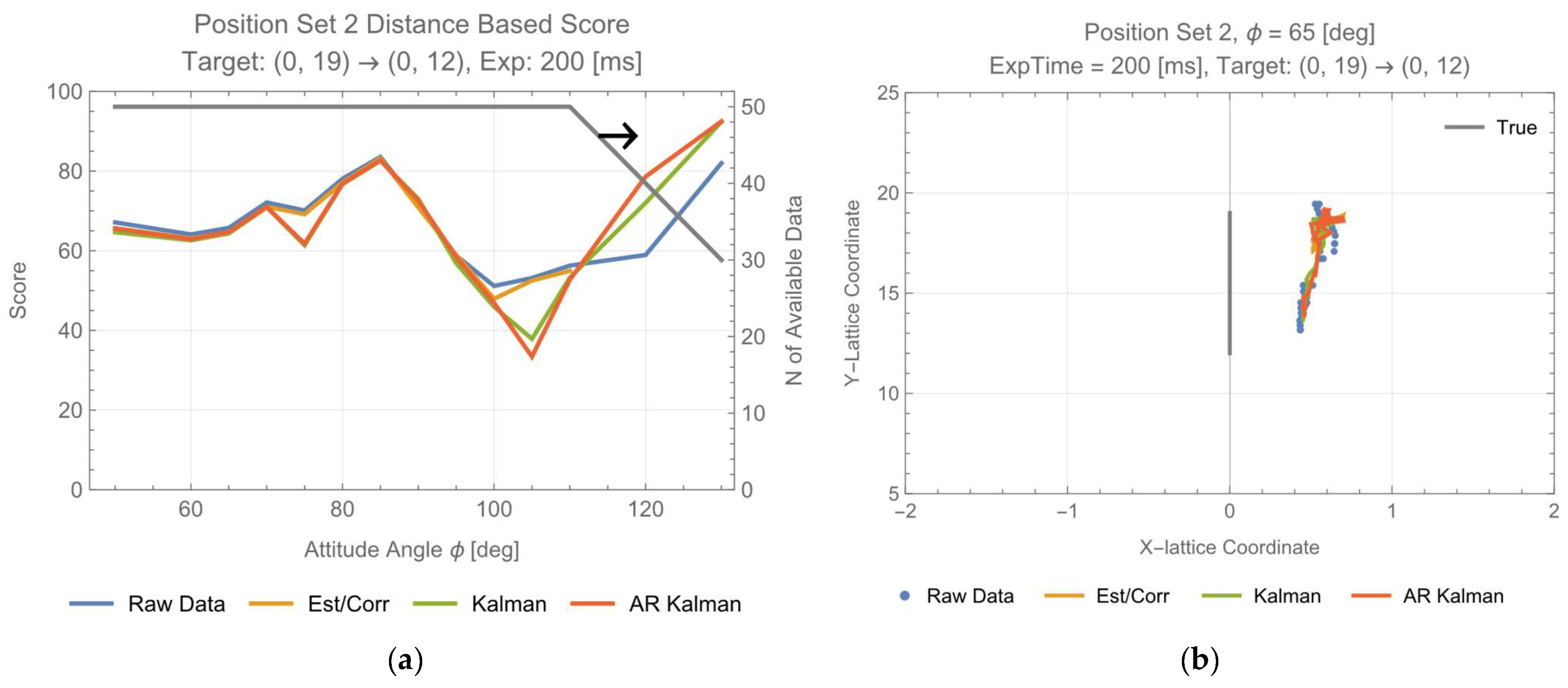
Figure 13 (position set 3). Along with the score evaluation results, the right vertical axis is showcased by the N (number) of available data which meet the integrity measure. Based on the plot, it appears that the values on the horizontal axis corresponding with the maximum values (=50) on the right vertical axis are near the normal direction, and that the scores seem to increase there. In Figure 12, position set 1 shows many outliers and missing data, suggesting that the correction by the algorithm is effective. However, since position set 3 data contain fewer outliers and missing data, the algorithm correction is limited in comparison with the raw data. Although the evaluation results of the three algorithms do not differ significantly, it seems that the estimator/corrector, which requires costs for additional training, behaves slightly superior to (the uniform motion/) Kalman filter and AR (model/) Kalman filter.

5. Discussion

5.1. Accuracy Improvement of the Three Algorithms

Figure 10 suggests that each position measurement accurately estimated ψ i near the normal, and this fact implies that ψ i can be regarded as a reliable (true) value there. The three algorithms in Section 4.1 estimated two coordinates x ,   y independently for position estimation. On the other hand, if we focus on the Y coordinate estimation and use it with the ‘reliable value’ ψ to calculate the X coordinate by x = y tan ψ , as shown in Figure 14, this estimation involves one estimation and one reliable value. In this case, improvement in accuracy is expected.
In this algorithm, the estimation error of ψ ( Δ ψ ) introduces an error in the score function S c o r e ( Δ S c o r e ). In situations where there is attitude angle deviation from the normal, the estimation of the direction may be subject to error. Δ S c o r e can be expressed as:
Δ S c o r e = S c o r e 2 100 1 N i = 1 N ( 2 y i   s e c ψ   t a n ψ ) Δ ψ
The value of Δ ψ is known to vary with the attitude angle ϕ, as illustrated in Figure 10. To evaluate Score and ΔScore, the results are shown in Figure 15, where ΔScore is represented as error bars.
Comparing Figure 15a with Figure 12a and Figure 15b with Figure 13b, there was a noticeable improvement in the scores for both cases. Despite the ranking of the three algorithms remaining largely consistent, estimator/corrector has a better average performance compared with both Kalman filter and AR Kalman filter.

5.2. Assessment of the Algorithms for Position Set 2

While the conclusion of Section 4.2.2 is supported by the data of position sets 1 and 3, there remains a question of whether the data of position set 2 also supports that.
For position set 2, while the improved method in Section 5.1 is applicable, evaluating the score using the method described in Section 4.2.1 to estimate the true value is not feasible. As an alternative, a possible method is to evaluate the target’s position error by measuring the distance between the estimated position and the true track instead of the true position. This method is referred to as distance-based score in this paper. This corresponds to using h I instead of e i in Figure 14, and, in other words, evaluating the score based solely on the cross-track error, ignoring the along-track error. From Figure 14, the following Equation (17) holds:
h i = e i s i n ω ψ
For position set 1, where ω = 90 deg and ψ < 5.7 (deg) (=0.1 (rad)), h i e i , and TP-based score and distance-based score are nearly identical. For position set 3, h i < e i , and distance-based score tends to overestimate. The track for position set 2 does not allow the application of Equation (17).
Figure 16 showcases the evaluation results of position estimation using the method in Section 5.1 and the scoring based on distance-based score.
Comparing Figure 15 and Figure 16, it can be concluded that the differences between them are minimal for position set 1, 3 data. Figure 17 presents the evaluation results of distance-based score for position set 2 data, where position estimation using the method in Section 5.1 was applied. Furthermore, the analysis results for additional data are added in Figure A1 and Figure A2 in Appendix A.
In position set 2, it is crucial to pay more attention to the impact of ignoring along-track errors in distance-based score. In Figure 17c, there exists a constant X direction error, but there does not seem to be any noticeable irregularity in the Y direction. Similarly, Figure 17b,d show random position errors in the X direction, but no observable random error in the Y direction. This suggests that the motion of the target along the Y axis is tracked appropriately. Based on the data, it can be inferred that the impact of ignoring along-track errors in position set 2 is allowable. This conclusion is also supported by the data in Figure A1 and Figure A2. Therefore, in position set 2, it is acceptable to evaluate the algorithms using distance-based score. When the three algorithms, modified according to Section 5.1, are assessed with distance-based score in position set 2, there is no significant difference in their performance.
Based on the discussion in Section 4.2.2 and above, it is concluded that, when there are many outliers and missing data, such as position set 1, the correction of outliers and interpolation of missing data by the algorithms are effective. Among the algorithms, estimator/corrector, which requires training costs, appears to be the best option as it outperforms both the Kalman filter and the AR Kalman filter. On the other hand, where there are fewer outliers and missing data, such as in position sets 2 and 3, the effect of the correction and the interpolation by the algorithms are limited, and the score of the measurements (raw data) may not be necessarily surpassed by the algorithms. In such cases, the performance of the three algorithms can be considered equivalent.

5.3. Consistency between System-Level Requirement Study

In the authors’ previous research, high-level requirement analysis for OWPT beam alignment and shaping was conducted. The overall power generation efficiency of the OWPT system ( η s y s t e m ) is expressed as:
η s y s t e m = η L i g h t   S o u r c e × η T r a n s m i s s i o n × η P o w e r   G e n e r a t i o n × η S o l a r C e l l
Among these, η L i g h t   S o u r c e , η S o l a r C e l l are device-dependent parameters, and η T r a n s m i s s i o n is a parameter that depends on the operating environment. η P o w e r   G e n e r a t i o n indicates the proportion of the beam energy incident on the PV that contributes to power generation [28]. The calculation method for η P o w e r   G e n e r a t i o n , including errors of the transmission optics is explained in a former research paper [6]. Figure 18 shows the analysis results for the X direction alignment error and power generation ratio in a cooperative OWPT system with a target size of 100 mm × 100 mm, which is used as a reference size in the former analysis [6]. From Figure 16 and Figure 17, the alignment error is estimated to be approximately 0.67 units or less. Figure 18 shows that the alignment error tolerance on the PV surface does not depend on the target distance, and that the power generation ratio can be greater than 55% for the estimated alignment error (≤0.67 unit = 17.0 mm).
It is worth noting that the accuracy depends on the exposure time of the image sensor, and that there is a minimum exposure time for the positioning accuracy to converge [13]. Because SNR is proportional to exposure time, it can be reworded that there is a minimum SNR for the positioning accuracy to converge. The SNR depends on several parameters; the formula was derived [11]. Since the target’s position is determined in the pixel coordinate system in this method, the resolution of the position estimation is determined by the angle of view of the pixel ( θ = 2.6 mrad/px). The further the target is, the smaller θ needs to be, thus the accuracy is limited by this parameter. The value ‘55%’ would be sufficient for an initial acquisition, and a high-resolution camera, a zoom lens, or enlarging the target size will be necessary to improve this.

6. Conclusions

This paper discussed real-time position and attitude estimation for moving targets.
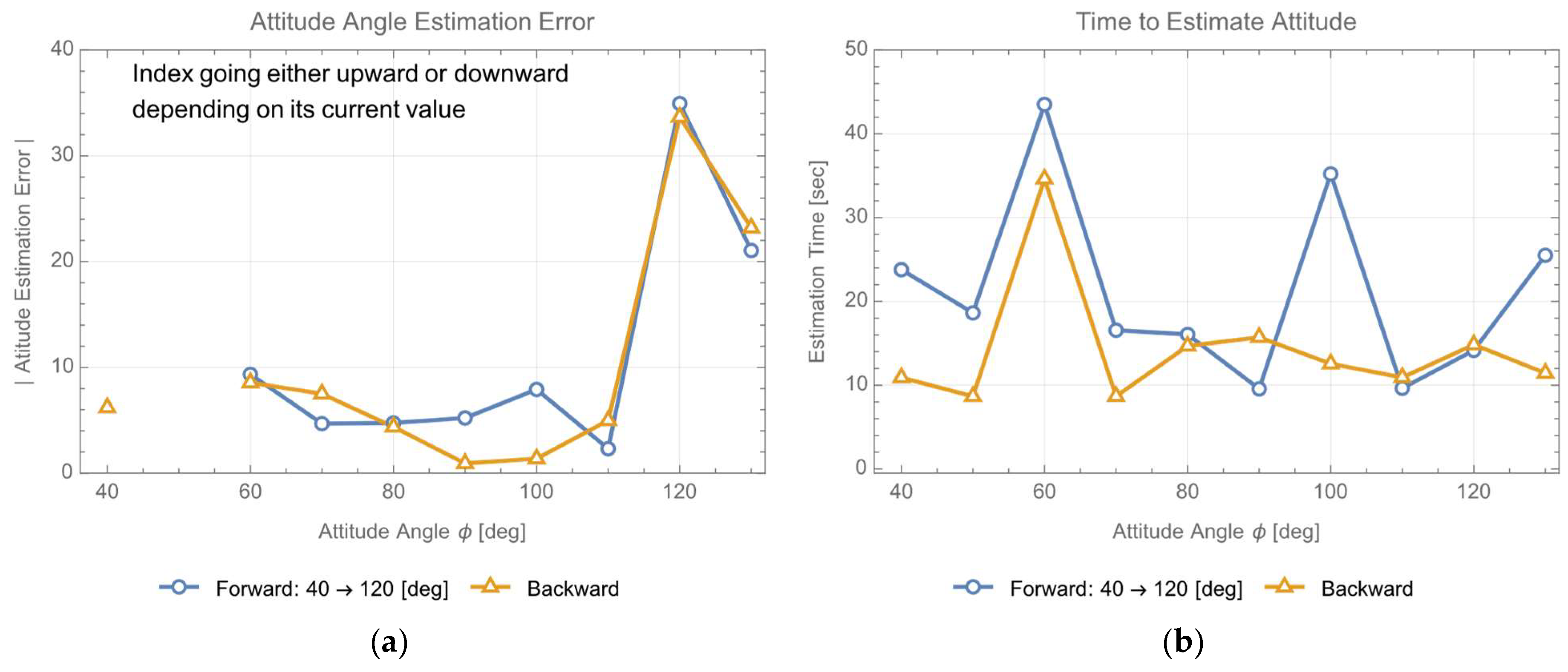
The target’s direction ψ can be accurately estimated with about ±0.15 deg (~±1 px) precision when it is near the normal. This feature can be used to improve the accuracy of position estimation by estimating the X coordinate as x = y   t a n ψ using Y coordinate estimation y and ψ . As a result, within the experiment set of 660 × 200 mm size, real-time tracking of the PV confirmed that the target positions were estimated within 17 mm error, and that its attitude was estimated within 10 deg error around the normal. It is worth noting that this accuracy can be improved by using a higher-resolution camera.
A score function based on the position estimation error can be used to compare three tracking algorithms. Position sets 1 and 3 allow for the estimation of true values using the azimuth angle ψ and the true track, enabling evaluation with true position (TP)-based score. For evaluation of position set 2 data, distance-based score based on the distance from the true track can be defined and rationally used. Based on the evaluation results of the score functions for the three algorithms, the estimator/corrector, a supervised model using AR models and thresholds, is generally superior, while there is little difference between the method of using the Kalman filter to estimate the position with a uniform motion model and the method of estimating the AR model with the Kalman filter. The choice of tracking algorithm depends on the system design. If a system allows for the training of a supervised algorithm, then choosing estimator/corrector would yield generally superior results, particularly near the normal position. However, if training is not an option, then choosing one of the algorithms using the Kalman filter should suffice.
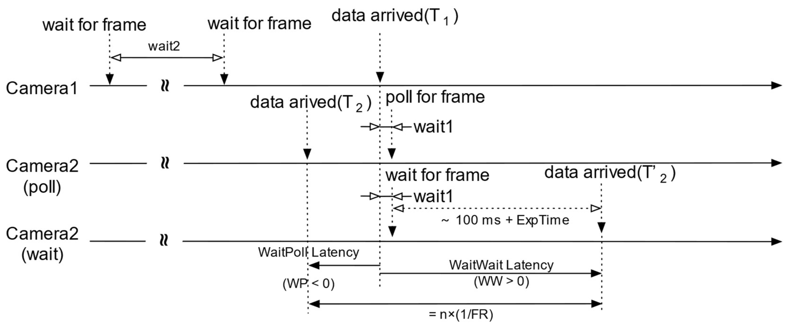
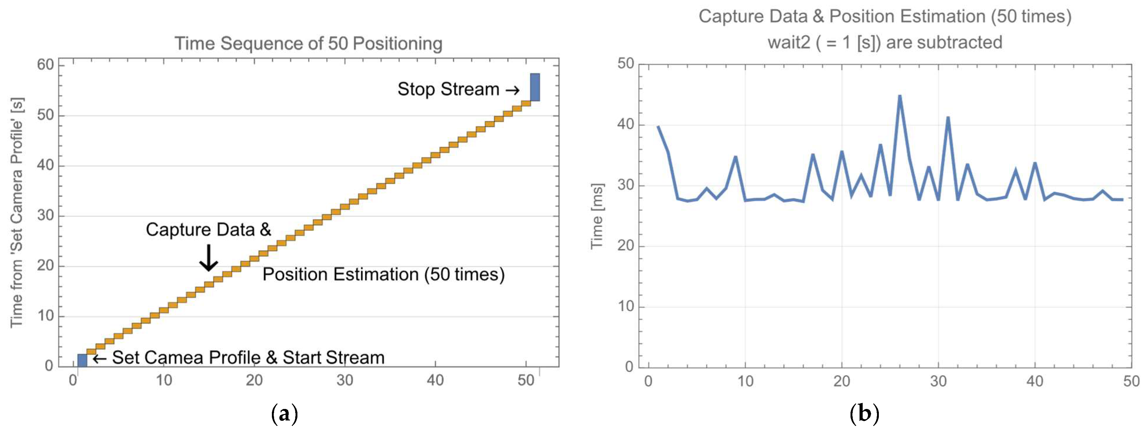
This paper investigated the necessary parameter settings for real-time position and attitude estimation based on an experimental setup that utilizes Intel D435. During the experiments, certain challenges related to the cameras were identified. To track the target and perform real-time position and attitude estimation, the initial configuration and the start/stop procedures for the camera must be executed within a short enough time relative to the camera’s data rate. Additionally, to minimize the latency between two cameras respectively corresponding to λ O N and λ O F F , hardware-based synchronization between the cameras is desirable. Suppose the time for the start/stop frame can be reduced from 8 s to 100 ms, the total time, including positioning and start/stop stream, is less than 125 ms. Such reduction, with the use of a high-speed PC, will generate attitude estimation data up to 4 Hz.
The detection and estimation of PV targets’ position and attitude angles are crucial for the implementation of OWPT systems. A series of studies by the authors have proposed a method addressing a unique and indispensable process for OWPT. From high-level requirements analysis in former research to target tracking in this paper, the conceptual verification of the method has been conducted. These works exhibit an advancement towards the practical implementation of OWPT systems.

Author Contributions

Conceptualization, K.A. and T.M.; methodology, K.A. and T.M.; formal analysis, K.A.; investigation, K.A.; data curation, K.A.; software, K.A.; writing—original draft preparation, K.A.; writing—review and editing, T.M.; project administration, T.M.; funding acquisition, T.M. All authors have read and agreed to the published version of the manuscript.

Funding

This work was partially supported by the Tsurugi-Photonics Foundation (No. 20220502) and the Takahashi Industrial and Economic Research Foundation (No. I2-003-13). In addition, part of this paper is based on the project commissioned by the Mechanical Social Systems Foundation and Optoelectronics Industry and Technology Development Association (“Formulation of strategies for market development of optical wireless power transmission systems for small mobilities”).

Institutional Review Board Statement

Not applicable.

Informed Consent Statement

Not applicable.

Data Availability Statement

Data are contained within the article.

Acknowledgments

The authors wish to thank Kenta Moriyama, members of the T. Miyamoto Lab for discussion and assistance, and Yota Suzuki of the Open Facility Center of Tokyo Institute of Technology for design support and manufacturing of the equipment for the experiments.

Conflicts of Interest

The authors declare no conflicts of interest.

Appendix A

Supporting data of position set 2.
Figure A1. Assessment of distance-based score for position set 2 with another data set, exp time = 200 (ms), (a) distance-based score; (b) data of ϕ = 75 (deg); (c) ϕ = 90 (deg); (d) ϕ = 95 (deg).
Photonics 11 00490 g0a1aPhotonics 11 00490 g0a1b
Figure A2. Assessment of distance-based score for position set 2 with another data set, exp time = 100 (ms), (a) distance-based score; (b) data of ϕ = 60 (deg); (c) ϕ = 70 (deg); (d) ϕ = 85 (deg).
Photonics 11 00490 g0a2

References

  1. Frolova, E.; Dobroskok, N.; Morozov, A. Critical Review of Wireless Electromagnetic Power Transmission Methods; Atlantis Press: Dordrecht, The Netherlands, 2022; pp. 14–20. [Google Scholar]
  2. Mohsan, S.A.H.; Othman, N.Q.H.; Khan, M.A.; Amjad, H.; Żywiołek, J. A Comprehensive Review of Micro UAV Charging Techniques. Micromachines 2022, 13, 977. [Google Scholar] [CrossRef] [PubMed]
  3. Qaraqe, M.; Usman, M.; Serbes, A.; Ansari, I.S.; Alouini, M.-S. Power Hotspots in Space: Powering CubeSats via Inter-Satellite Optical Wireless Power Transfer. IEEE Internet Things Mag. 2022, 5, 180–185. [Google Scholar] [CrossRef]
  4. Marcinkowski, A.; Carrio, L.; Hilliard, S.; Edwards, C.; Elhawary, A.; Clem, D.; Blood, M.; May, L.; Cichan, T. Lunar Surface Power Architecture Concepts. In Proceedings of the 2023 IEEE Aerospace Conference, Big Sky, MT, USA, 4–11 March 2023; pp. 1–19. [Google Scholar]
  5. Technologies, P. PowerLight Ships the First Long Distance Power over Fiber Prototype for Powering Telecom 5G Networks to a Major US Telecom; PowerLight Technologies: Kent, WA, USA, 2023. [Google Scholar]
  6. Asaba, K.; Miyamoto, T. System Level Requirement Analysis of Beam Alignment and Shaping for Optical Wireless Power Transmission System by Semi–Empirical Simulation. Photonics 2022, 9, 452. [Google Scholar] [CrossRef]
  7. GPS.Gov: GPS Accuracy. Available online: https://www.gps.gov/systems/gps/performance/accuracy/ (accessed on 9 May 2022).
  8. Indoor Positioning System. Available online: https://www.quuppa.com/indoor-positioning-system/ (accessed on 9 May 2022).
  9. Setiawan Putra, A.W.; Kato, H.; Maruyama, T. Infrared LED Marker for Target Recognition in Indoor and Outdoor Applications of Optical Wireless Power Transmission System. Jpn. J. Appl. Phys. 2020, 59, SOOD06. [Google Scholar] [CrossRef]
  10. Imai, H.; Watanabe, N.; Chujo, K.; Hayashi, H.; Yamauchi, A. Beam-Tracking Technology Developed for Free-Space Optical Communication and Its Application to Optical Wireless Power Transfer. In Proceedings of the 4th Optical Wireless and Fiber Power Transmission Conference (OWPT2022), Yokohama, Japan, 18–21 April 2022. [Google Scholar]
  11. Asaba, K.; Moriyama, K.; Miyamoto, T. Preliminary Characterization of Robust Detection Method of Solar Cell Array for Optical Wireless Power Transmission with Differential Absorption Image Sensing. Photonics 2022, 9, 861. [Google Scholar] [CrossRef]
  12. Asaba, K.; Miyamoto, T. Solar Cell Detection and Position, Attitude Determination by Differential Absorption Imaging in Optical Wireless Power Transmission. Photonics 2023, 10, 553. [Google Scholar] [CrossRef]
  13. Asaba, K.; Miyamoto, T. Positioning of a Photovoltaic Device on a Real Two-Dimensional Plane in Optical Wireless Power Transmission by Means of Infrared Differential Absorption Imaging. Photonics 2023, 10, 1111. [Google Scholar] [CrossRef]
  14. Asaba, K.; Miyamoto, T. Attitude Determination of Photovoltaic Device by Means of Differential Absorption Imaging. Photonics 2023, 11, 32. [Google Scholar] [CrossRef]
  15. Intel® RealSenseTM. Available online: https://www.intelrealsense.com/sdk-2/ (accessed on 24 August 2022).
  16. Welcome to Python.Org. Available online: https://www.python.org/ (accessed on 24 August 2022).
  17. Wolfram Mathematica: Modern Technical Computing. Available online: https://www.wolfram.com/mathematica/ (accessed on 15 August 2022).
  18. Hardware and Software Synchronization—Realsense Multicam · Issue #11669 · IntelRealSense/Librealsense. Available online: https://github.com/IntelRealSense/librealsense/issues/11669 (accessed on 10 February 2024).
  19. API How-To. Available online: https://dev.intelrealsense.com/docs/api-how-to (accessed on 20 February 2024).
  20. Difference between ‘poll_for_frames’ and ‘wait_for_frames’ Modes? · Issue #2422 · IntelRealSense/Librealsense · GitHub. Available online: https://github.com/IntelRealSense/librealsense/issues/2422 (accessed on 20 February 2024).
  21. Montgomery, D.C.; Jennings, C.L.; Kulahci, M. Introduction to Time Series Analysis and Forecasting, 2nd ed.; John Wiley & Sons: Hoboke, NJ, USA, 2015; ISBN 978-1-118-74511-3. [Google Scholar]
  22. Chandola, V.; Banerjee, A.; Kumar, V. Anomaly Detection: A Survey. ACM Comput. Surv. 2009, 41, 1–58. [Google Scholar] [CrossRef]
  23. Oppenheim, A.V.; Schafer, R.W. Digital Singal Processing; Prentice-Hall: Englewood Cliffs, NJ, USA, 1975; ISBN 0-13-214635-5. [Google Scholar]
  24. Haykin, S. Adaptive Filter Theory, 2nd ed.; Prentice-Hall: Englewood Cliffs, NJ, USA, 1991; ISBN 0-13-005513-1. [Google Scholar]
  25. Jones, R.H. Maximum Likelihood Fitting of ARMA Models to Time Series with Missing Observations. Technometrics 1980, 22, 389–395. [Google Scholar] [CrossRef]
  26. Zhou, X.; Zhao, Y.; Zhuang, X. Kalman Filter Channel Tracking Algorithm Based on AR Model in WCDMA Systems. In Proceedings of the WCC 2000—ICSP 2000, 2000 5th International Conference on Signal Processing Proceedings, 16th World Computer Congress 2000, Beijing, China, 21–25 August 2000; Volume 3, pp. 1759–1762. [Google Scholar]
  27. Tatinati, S.; Veluvolu, K.C.; Hong, S.-M.; Latt, W.T.; Ang, W.T. Physiological Tremor Estimation With Autoregressive (AR) Model and Kalman Filter for Robotics Applications. IEEE Sens. J. 2013, 13, 4977–4985. [Google Scholar] [CrossRef]
  28. Tang, J.; Matsunaga, K.; Miyamoto, T. Numerical Analysis of Power Generation Characteristics in Beam Irradiation Control of Indoor OWPT System. Opt. Rev. 2020, 27, 170–176. [Google Scholar] [CrossRef]
Figure 1. Configuration of the experiments.
Photonics 11 00490 g001
Figure 2. Position estimation by stereo imagery.
Photonics 11 00490 g002
Figure 3. Timing chart of camera 1 and camera 2.
Photonics 11 00490 g003
Figure 4. Frame rate estimation.
Photonics 11 00490 g004
Figure 5. Camera 1 → camera 2 latency, (a) latency (wait1 = 18 (ms), exp time = 200 (ms)); (b) Max–min latency of 50 successive data, normalized by exp time.
Photonics 11 00490 g005
Figure 6. Time sequence of 50 successive position estimations. (a) The whole sequence (wait1 = 18 (ms), exp time = 200 (ms)). (b) Time for capture and position estimation (50 data).
Photonics 11 00490 g006
Figure 7. Moving target experiments. (a) Layout of experiments (position set 1). (b) Position set 1 data.
Photonics 11 00490 g007
Figure 8. Successive attitude determination of the PV. (a) The attitude estimation error. (b) The time to estimate the attitude.
Photonics 11 00490 g008
Figure 9. Tracking of the PV target, (ac) position sets 1, 2, and 3.
Photonics 11 00490 g009
Figure 10. Direction angle estimation accuracy.
Photonics 11 00490 g010
Figure 11. True position estimation by direction angle ψ .
Photonics 11 00490 g011
Figure 12. Assessment of the three algorithms by TP-based score for position set 1, (a) TP-based score; (b) data of ϕ = 90 (deg); (c) ϕ = 95 (deg); (d) ϕ = 100 (deg).
Photonics 11 00490 g012aPhotonics 11 00490 g012b
Figure 13. Assessment of the three algorithms by TP-based score for position set 3, (a) TP-based score; (b) data of ϕ = 70 (deg); (c) ϕ = 75 (deg); (d) ϕ = 85 (deg).
Photonics 11 00490 g013
Figure 14. Position estimation by direction angle ψ .
Photonics 11 00490 g014
Figure 15. Assessment of the three improved algorithms by TP-based score, (a) position set 1; (b) position set 3.
Photonics 11 00490 g015
Figure 16. Assessment of the three improved algorithms by distance-based score, (a) position set 1; (b) position set 3.
Photonics 11 00490 g016
Figure 17. Assessment of the three algorithms by distance-based score for position set 2, (a) distance-based score; (b) data of ϕ = 75 (deg); (c) ϕ = 90 (deg); (d) ϕ = 95 (deg).
Photonics 11 00490 g017aPhotonics 11 00490 g017b
Figure 18. Power generation ratio and X alignment error.
Photonics 11 00490 g018
Table 1. Parameters in the experiments.
LED power 2   mW   ×   2   for   λ = 850 nm and 940 nm
GaAs substrate2-inch diameter
GaAs PV6 cm × 4 cm
Distance from the camera assembly660 mm (typical)
Attitude angle43~123 deg (typical)
CameraIntel D435TM × 2
Exposure time25, 50, 100, 250, 500, 1000, 2500, 5000, 10,000, 25,000, 50,000, 100,000 and 200,000 μ s
Image size640 × 480 px
Disclaimer/Publisher’s Note: The statements, opinions and data contained in all publications are solely those of the individual author(s) and contributor(s) and not of MDPI and/or the editor(s). MDPI and/or the editor(s) disclaim responsibility for any injury to people or property resulting from any ideas, methods, instructions or products referred to in the content.

