Single-Shot Fringe Projection Profilometry Based on LC-SLM Modulation and Polarization Multiplexing


Abstract
1. Introduction
2. Materials and Methods
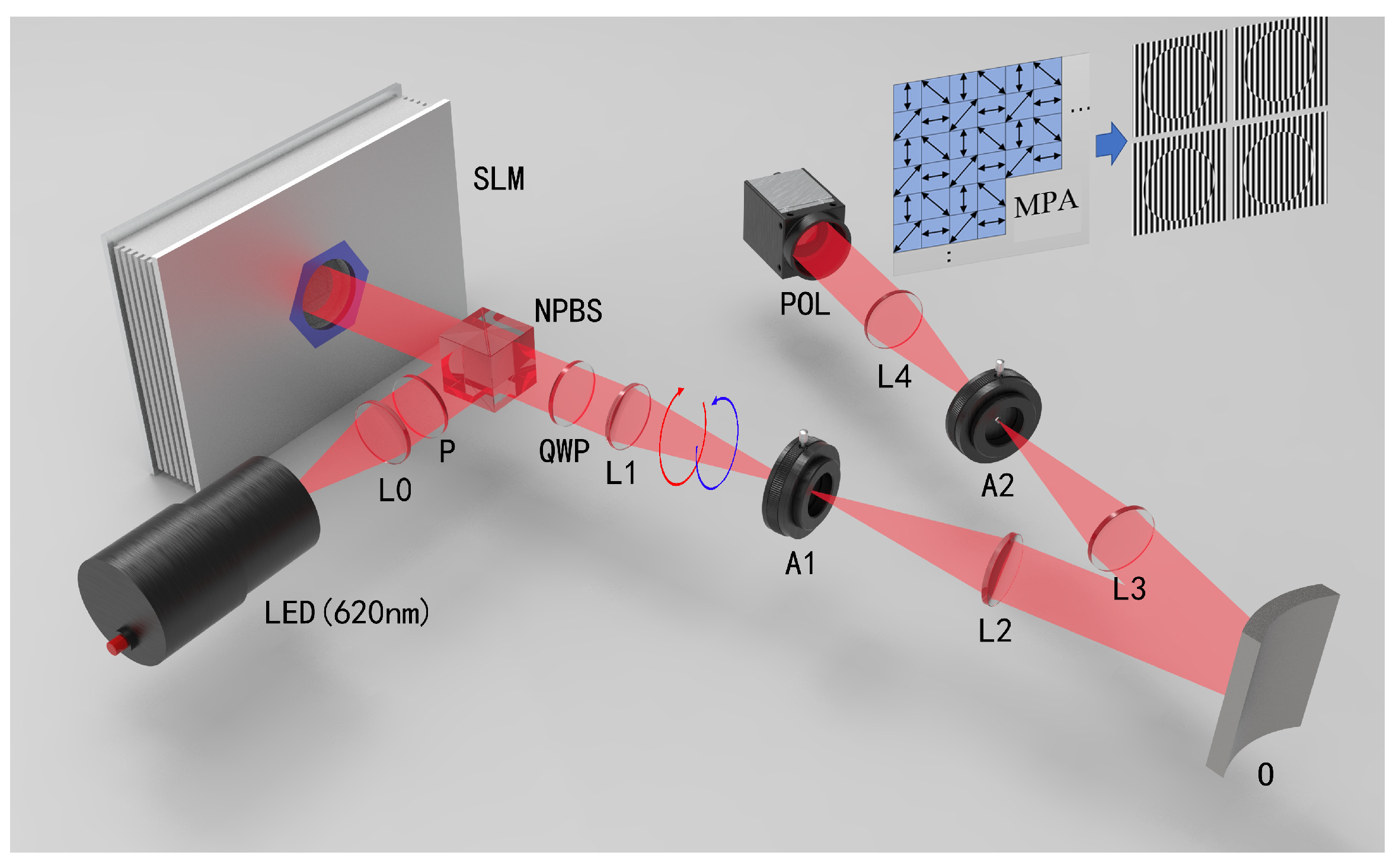
2.1. Principle of Optical System
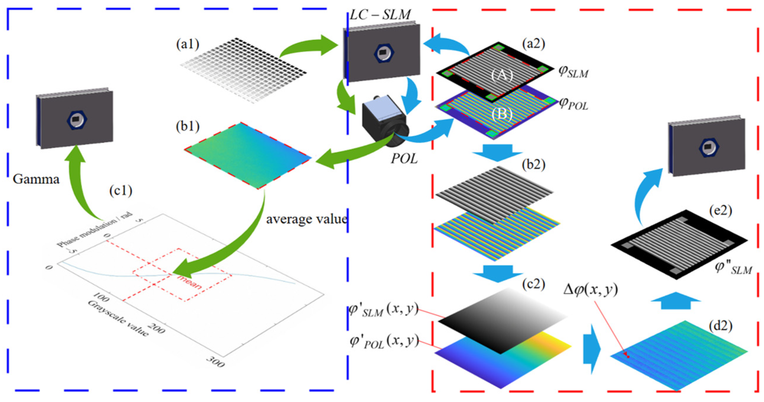
2.2. Phase Calibration of LC-SLM
3. Results
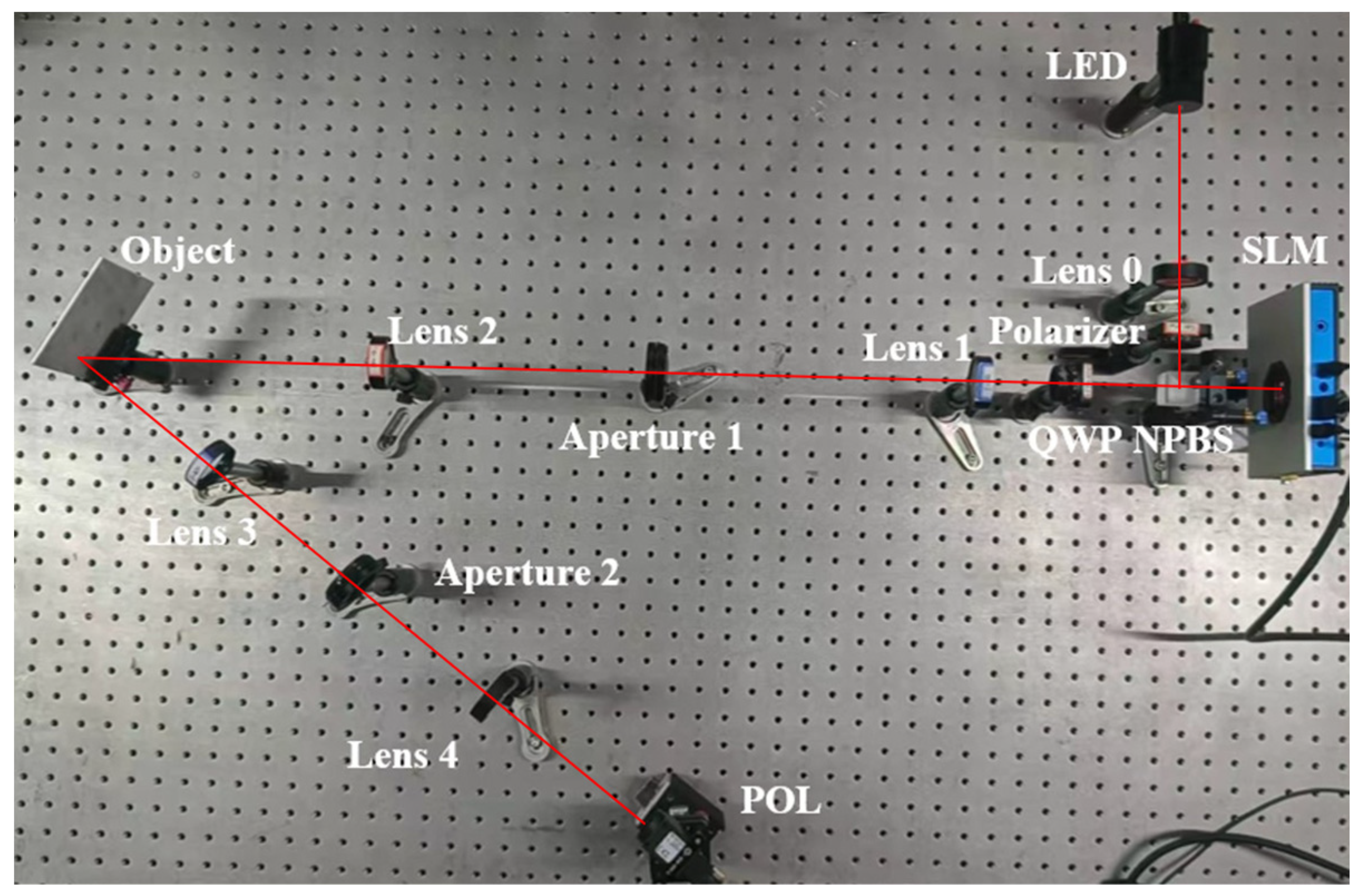
3.1. Optical System
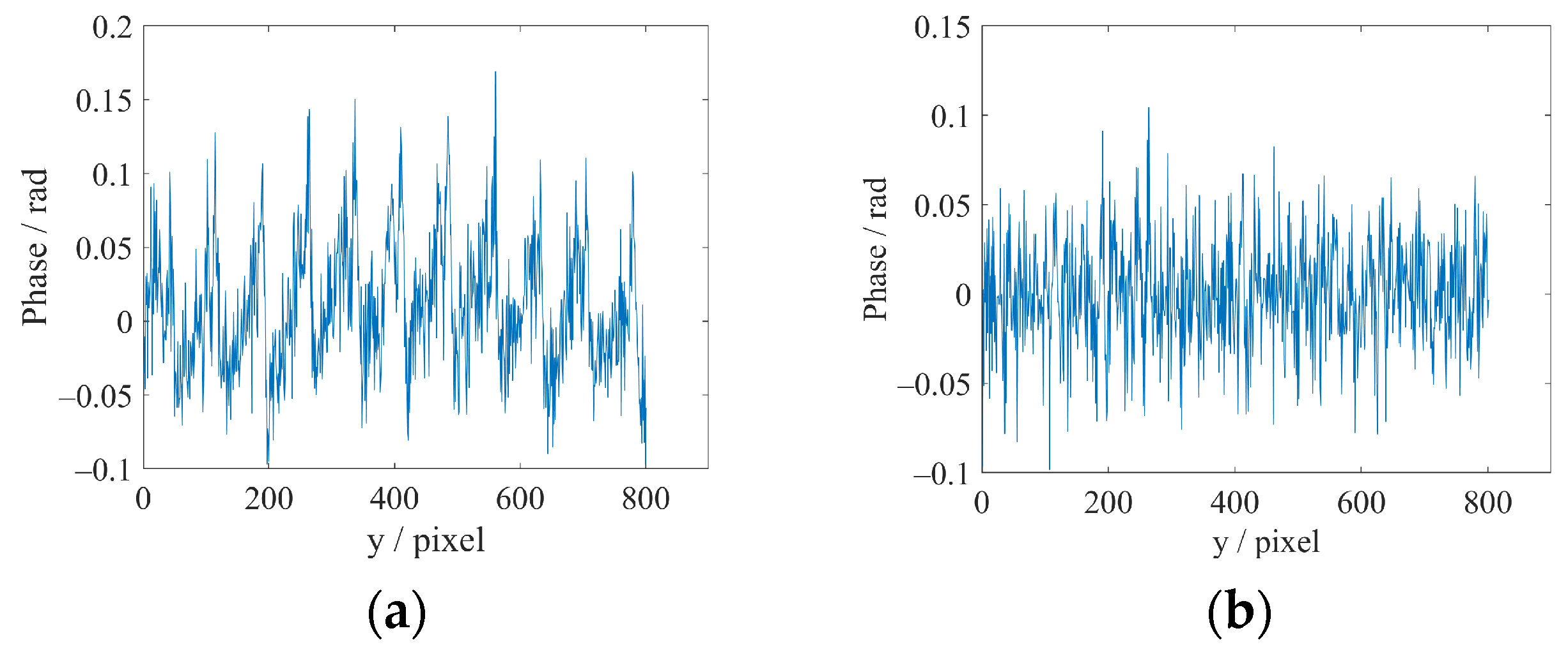
3.2. LC-SLM Nonlinear Correction Experiment
3.3. Sample Measurement
4. Discussion
5. Conclusions
Author Contributions
Funding
Institutional Review Board Statement
Informed Consent Statement
Data Availability Statement
Conflicts of Interest
References
- Cai, Z.; Liu, X.; Peng, X.; Yin, Y.; Li, A.; Wu, J.; Gao, B.Z. Structured light field 3D imaging. Opt. Express 2016, 24, 20324–20334. [Google Scholar] [CrossRef] [PubMed]
- Fu, Y.; Luo, Q. Fringe projection profilometry based on a novel phase shift method. Opt. Express 2011, 19, 21739–21747. [Google Scholar] [CrossRef]
- Strand, T.C. Optical three-dimensional sensing for machine vision. Opt. Eng. 1985, 24, 240133. [Google Scholar] [CrossRef]
- Duan, M.; Jin, Y.; Xu, C.; Xu, X.; Zhu, C.; Chen, E. Phase-shifting profilometry for the robust 3-D shape measurement of moving objects. Opt. Express 2019, 27, 22100–22115. [Google Scholar] [CrossRef] [PubMed]
- Zhang, Z.; Huang, S.; Meng, S.; Gao, F.; Jiang, X. A simple, flexible and automatic 3D calibration method for a phase calculation-based fringe projection imaging system. Opt. Express 2013, 21, 12218–12227. [Google Scholar] [CrossRef]
- Srinivasan, V.; Liu, H.C.; Halioua, M. Automated phase-measuring profilometry of 3-D diffuse objects. Appl. Opt. 1984, 23, 3105–3108. [Google Scholar] [CrossRef]
- Takeda, M.; Mutoh, K. Fourier transform profilometry for the automatic measurement of 3-D object shapes. Appl. Opt. 1983, 22, 3977–3982. [Google Scholar] [CrossRef]
- Kemao, Q. Two-dimensional windowed Fourier transform for fringe pattern analysis: Principles, applications and implementations. Opt. Lasers Eng. 2007, 45, 304–317. [Google Scholar] [CrossRef]
- Zhong, J.; Weng, J. Phase retrieval of optical fringe patterns from the ridge of a wavelet transform. Opt. Lett. 2005, 30, 2560–2562. [Google Scholar] [CrossRef]
- Huang, L.; Kemao, Q.; Pan, B.; Asundi, A.K. Comparison of Fourier transform, windowed Fourier transform, and wavelet transform methods for phase extraction from a single fringe pattern in fringe projection profilometry. Opt. Lasers Eng. 2010, 48, 141–148. [Google Scholar] [CrossRef]
- Liu, H.; Yan, N.; Shao, B.; Yuan, S.; Zhang, X. Deep Learning in Fringe Projection: A Review. Neurocomputing 2024, 581, 127493. [Google Scholar] [CrossRef]
- Wang, C.; Zhou, P.; Zhu, J. Deep learning-based end-to-end 3D depth recovery from a single-frame fringe pattern with the MSUNet++ network. Opt. Express 2023, 31, 33287–33298. [Google Scholar] [CrossRef] [PubMed]
- Feng, S.; Chen, Q.; Gu, G.; Tao, T.; Zhang, L.; Hu, Y.; Yin, W.; Zuo, C. Fringe pattern analysis using deep learning. Adv. Photonics 2019, 1, 025001. [Google Scholar] [CrossRef]
- Zheng, Y.; Wang, S.; Li, Q.; Li, B. Fringe projection profilometry by conducting deep learning from its digital twin. Opt. Express 2020, 28, 36568–36583. [Google Scholar] [CrossRef]
- Liu, B.; Wang, C.; Wang, S.; Wu, G. Color crosstalk compensation method for color phase-shifting fringe projection profilometry based on the phase correction matrix. Opt. Express 2024, 32, 5793–5808. [Google Scholar] [CrossRef]
- Zhu, Q.; Zhao, H.; Zhao, Z. Research on iterative decoupling algorithm in color fringe projection profilometry. Opt. Laser Technol. 2023, 164, 109541. [Google Scholar] [CrossRef]
- Wan, Y.; Cao, Y.; Liu, X.; Tao, T.; Kofman, J. High-frequency color-encoded fringe-projection profilometry based on geometry constraint for large depth range. Opt. Express 2020, 28, 13043–13058. [Google Scholar] [CrossRef]
- Zhang, Z.; Towers, D.P.; Towers, C.E. Snapshot color fringe projection for absolute three-dimensional metrology of video sequences. Appl. Opt. 2010, 49, 5947–5953. [Google Scholar] [CrossRef]
- Zhang, Z.; Towers, C.E.; Towers, D.P. Time efficient color fringe projection system for 3D shape and color using optimum 3-frequency selection. Opt. Express 2006, 14, 6444–6455. [Google Scholar] [CrossRef]
- Zhou, X.; Jia, S.; Zhang, H.; Lin, Z.; Wen, B.; Wang, L.; Zhang, Y. Single-frame fringe pattern analysis with synchronous phase-shifting based on polarization interferometry phase measuring deflectometry (PIPMD). Opt. Lasers Eng. 2024, 181, 108406. [Google Scholar] [CrossRef]
- Chen, Z.; Wang, X.; Liang, R. Snapshot phase shift fringe projection 3D surface measurement. Opt. Express 2015, 23, 667–673. [Google Scholar] [CrossRef] [PubMed]
- Zhao, Z.; Zhang, H.; Xiao, Z.; Du, H.; Zhuang, Y.; Fan, C.; Zhao, H. Robust 2D phase unwrapping algorithm based on the transport of intensity equation. Meas. Sci. Technol. 2018, 30, 015201. [Google Scholar] [CrossRef]
- Du, Y.; Li, J.; Fan, C.; Yang, X.; Zhao, Z.; Zhao, H. Dynamic three-dimensional deformation measurement by polarization-multiplexing of full complex amplitude. Opt. Express 2024, 32, 11737–11750. [Google Scholar] [CrossRef]
- Rodriguez-Zurita, G.; Meneses-Fabian, C.; Toto-Arellano, N.I.; Vázquez-Castillo, J.F.; Robledo-Sánchez, C. One-shot phase-shifting phase-grating interferometry with modulation of polarization: Case of four interferograms. Opt. Express 2008, 16, 7806–7817. [Google Scholar] [CrossRef] [PubMed]
- Novak, M.; Millerd, J.; Brock, N.; North-Morris, M.; Hayes, J.; Wyant, J. Analysis of a micropolarizer array-based simultaneous phase-shifting interferometer. Appl. Opt. 2005, 44, 6861–6868. [Google Scholar] [CrossRef] [PubMed]
- Guo, W.; Wu, Z.; Zhang, Q.; Wang, Y. Real-time motion-induced error compensation for 4-step phase-shifting profilometry. Opt. Express 2021, 29, 23822–23834. [Google Scholar] [CrossRef]
- Shan, X.; Duan, M.; Ai, Y.; Hu, L. Calibration approaches of the phase nonlinearity of the phase-only liquid crystal spatial light modulator. Acta Photonica Sin. 2014, 43, 0623001. [Google Scholar] [CrossRef]
- Otón, J.; Ambs, P.; Millán, M.S.; Pérez-Cabré, E. Multipoint phase calibration for improved compensation of inherent wavefront distortion in parallel aligned liquid crystal on silicon displays. Appl. Opt. 2007, 46, 5667–5679. [Google Scholar] [CrossRef]


Disclaimer/Publisher’s Note: The statements, opinions and data contained in all publications are solely those of the individual author(s) and contributor(s) and not of MDPI and/or the editor(s). MDPI and/or the editor(s) disclaim responsibility for any injury to people or property resulting from any ideas, methods, instructions or products referred to in the content. |
© 2024 by the authors. Licensee MDPI, Basel, Switzerland. This article is an open access article distributed under the terms and conditions of the Creative Commons Attribution (CC BY) license (https://creativecommons.org/licenses/by/4.0/).
Share and Cite
Shu, L.; Li, J.; Du, Y.; Fan, C.; Hu, Z.; Chen, H.; Zhao, H.; Zhao, Z. Single-Shot Fringe Projection Profilometry Based on LC-SLM Modulation and Polarization Multiplexing. Photonics 2024, 11, 994. https://doi.org/10.3390/photonics11110994
Shu L, Li J, Du Y, Fan C, Hu Z, Chen H, Zhao H, Zhao Z. Single-Shot Fringe Projection Profilometry Based on LC-SLM Modulation and Polarization Multiplexing. Photonics. 2024; 11(11):994. https://doi.org/10.3390/photonics11110994
Chicago/Turabian StyleShu, Long, Junxiang Li, Yijun Du, Chen Fan, Zirui Hu, Huan Chen, Hong Zhao, and Zixin Zhao. 2024. "Single-Shot Fringe Projection Profilometry Based on LC-SLM Modulation and Polarization Multiplexing" Photonics 11, no. 11: 994. https://doi.org/10.3390/photonics11110994
APA StyleShu, L., Li, J., Du, Y., Fan, C., Hu, Z., Chen, H., Zhao, H., & Zhao, Z. (2024). Single-Shot Fringe Projection Profilometry Based on LC-SLM Modulation and Polarization Multiplexing. Photonics, 11(11), 994. https://doi.org/10.3390/photonics11110994