Abstract
The tip–tilt mirror (TTM) is an important component of adaptive optics (AO) to achieve beam stabilization and pointing tracking. In many practical applications, the information of accurate TTM dynamics, complete system state, and noise characteristics is difficult to achieve due to the lack of sufficient sensors, which then restricts the implementation of high precision tracking control for TTM. To this end, this paper proposes a new method based on noisy-output feedback Q-learning. Without relying on neural networks or additional sensors, it infers the dynamics of the controlled system and reference jitter using only noisy measurements, thereby achieving optimal tracking control for the TTM system. We have established a modified Bellman equation based on estimation theory, directly linking noisy measurements to system performance. On this basis, a fast iterative learning of the control law is implemented through the adaptive transversal predictor and experience replay technique, making the algorithm more efficient. The proposed algorithm has been validated with an application to a TTM tracking control system, which is capable of quickly learning near-optimal control law under the interference of random noise. In terms of tracking performance, the method reduces the tracking error by up to 98.7% compared with the traditional integral control while maintaining a stable control process. Therefore, this approach may provide an intelligent solution for control issues in AO systems.
1. Introduction
The tip–tilt mirror (TTM) tracking control system is one of the most important components of the adaptive optics (AO) system, which is primarily used in various optical systems to compensate for beam jitter caused by the atmosphere, mechanical vibrations, and other factors in the optical path. The aim is to achieve beam stabilization and enhance the pointing accuracy or imaging quality of the system [1,2,3]. Although the traditional integral controllers most used in TTM systems are simple in design and stable, they have limited control bandwidth, and thus it is increasingly difficult to satisfy the system’s needs in increasingly complex application scenarios. With the advancement of artificial intelligence (AI), many studies have integrated machine learning techniques into system control schemes to establish intelligent systems and enhance performance [4,5,6]. The authors in [7] developed a reinforcement learning (RL) method based on recurrent neural networks (RNNs) for jitter suppression in TTM systems, achieving control performance superior to that of the optimal gain integrator. However, most existing machine learning-based methods focus on the development of neural networks as the key to controller design, and complex network models require a large amount of sampling data and time consumption during training, which is not conducive to the application needs of practical systems.
In order to implement a simpler and more efficient reinforcement learning method in the system, Werbos [8] attempted to interpret the reinforcement learning concept from the perspective of optimal control computation and proposed the Adaptive Dynamic Programming (ADP) algorithm. Compared to traditional deep reinforcement learning algorithms, the ADP method provides a convex optimization control index and replaces the slow update of neural networks with efficient iterative numerical solutions, greatly improving the efficiency and stability of the algorithm. This makes ADP-based RL a powerful tool for solving the dynamic optimal control problems of unknown systems (including optimal tracking control) [9,10,11]. And therefore, the research based on ADP-based RL has been widely carried out in simulated systems such as autonomous vehicles [12,13], energy systems [14,15], and robot control [16,17]. However, in many of the TTM systems, there are two more factors that affect the design and performance of a controller except for the unknown dynamics. The first is the unmeasurable system state. The complexity of real systems and the absence of matching sensors results in incomplete system state information, making it tough to control such partially observed Markov decision processes (POMDPs) [18] through standard state feedback methods. The second one is the stochastic noise introduced by the sensors or by the environment, which requires us to analyze the problem from the perspective of stochastic system control.
On the one hand, in addressing scenarios with unmeasurable state information, numerous studies have leveraged neural networks for state estimation instead of traditional full-state observers [19,20,21]. Despite their ability to capture system nonlinearities, these networks require meticulous design to ensure stability and a large amount of training time for convergency. Alternative approaches [22,23,24] focus on output feedback (OPFB), enabling linear state reconstruction from input–output data, thereby facilitating optimal control outcomes without estimation errors. The aforementioned methods, while showing progress in managing unmeasurable states, are tailored for deterministic systems. Those methods that rely on input–output data for system state reconstruction will become ineffective when measurement data are corrupted by stochastic noise. This susceptibility to noise significantly restricts their applicability in practical scenarios, where both measurement and computational noise are inherent.
On the other hand, for the control problem of stochastic systems containing noise, a system transformation method was applied in [25] to convert the stochastic linear-quadratic (SLQ) control problem with signal-dependent noise into a deterministic framework. The authors of [26] introduced an optimistic least-squares policy iteration (O-LSPI) strategy for controlling linear stochastic systems subjected to additive noise. Furthermore, the control challenges for stochastic systems with both signal-dependent and additive noise have been studied in [27,28]. To deal with stochastic systems with unmeasurable state, the authors of [29] designed a data-driven two-stage control strategy to obtain the optimal observer and optimal controller, respectively. It is worth noting that only signal-dependent noise is considered in [25], while actual measurement noise is typically additive in nature. The system state is assumed to be known in [26,28], and the work in [20,27] relies on the assumption that the noise is measurable.
The TTM systems are typically stochastic systems that simultaneously contain unknown noise and unmeasurable state. The above discussion implies that it still remains a challenge to design optimal controllers for TTM systems using only noisy input–output data when both the system state and the noise information are unavailable. Motivated by this, this paper develops an improved RL-based tracking control scheme for TTM systems. To the best of our knowledge, there is currently little relevant research on this issue, which means that our work has greater potential and advantage in solving tracking control problems in practice. We validate the effectiveness of the scheme to achieve tracking control in a TTM system. The main contributions of the proposed scheme are summarized as follows:
- A RL-based noisy-OPFB Q-learning scheme is proposed, which achieves a rapid and effective solution for the near optimal tracking controller according to state estimation theory, transversal prediction, and experience replay techniques.
- In contrast to the works in [25,27,28], the additive noise independent of state and inputs are taken into account, and the measurable assumption of full state or noise information is removed; only measured input–output data are used during the entire learning process. Also, an additional state observation step is not required, so it is more convenient to implement than the methods in [29].
- The effectiveness of the algorithm is demonstrated through an application example in a TTM tracking control system. Meanwhile, the application prospects of the method in the control of intelligent optical systems have been illustrated by a comparison with the traditional integral controller.
The remainder of this paper is organized as follows: The problem and some preliminaries are stated in Section 2. Section 3 describes the main development of this paper, where a noisy-OPFB Q-learning scheme for stochastic linear quadratic tracking systems is established. Section 4 presents a TTM tracking control system that demonstrates the effectiveness of the proposed algorithm through numerical application examples and analysis. Finally, some concluding remarks are summarized in Section 5.
2. Problem Formulation
A schematic diagram of a classic TTM control system is shown in Figure 1. The far-field camera detects the positional error of the focused spot and feeds it back to the controller. The controller calculates the control voltage and drives the TTM to rapidly deflect the mirror in the opposite direction, compensating for the beam jitter. In principle, this process can also be seen as a tracking control of the beam jitter signal. It can be seen that without adding additional sensors, the system can only obtain the tracking error signal contaminated by the camera’s stochastic noise. The model and state information of the controlled TTM system and the reference jitter signal are unknown, and the noise is unmeasurable. Therefore, designing a stochastic optimal tracking controller under these conditions is challenging.
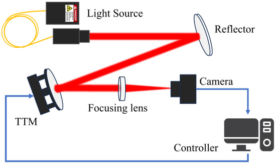
Figure 1.
Schematic diagram of a classic TTM tracking control system.
Consider the representation of the above TTM system as a state space model of the form
where is the unknown system state, is the control input, and is the system output; for simplicity, we assume . A, B, and C are unknown system matrices with proper dimensions. and are uncorrelated zero-mean Gaussian white noise with their semi-positive defined covariance matrices denoted as W1 and V. In addition, this TTM system is considered to have a time delay of two frames.
The time delay of system (1) reflects the aftereffect of the control input; we could rewrite the time delay system in a delay-free form using state augmentation. By combining the delayed inputs with the original state, the augmented state can be obtained as , and the delay-free system is
The beam jitter signal to be tracked by system (1) can be expressed in the following reference trajectory model:
where is the state of system (1). and are unknown constant matrices.
Remark 1.
System (3) is known as a command generator model [30], where E is not required to be Hurwitz. Such a model is able to generate many common trajectories, such as sinusoidal signals, square waveforms, the ramp, and so on.
Without loss of generality, we give the following assumptions: , the pair is controllable, and and are observable. Considering the system model (1) and the reference trajectory model (3), the following augmented system can be constructed:
where the augmented state is , is the augmented noise term with its covariance matrix , and is the augmented system output, which represents the tracking error.
For jitter tracking and suppression in TTM systems, the stochastic optimal tracking problem aims to find an optimal feedback control sequence to minimize the following cost function:
where is a discount factor, which is necessary here to make sure that is bounded even though disturbed by noises. and are symmetric weight matrices, respectively; and are observable. The cost function (5) is also known as the value function.
Under given assumptions, it is clear that when noise terms and are not considered, the problem mentioned above degenerates into the infinite-horizon linear quadratic tracking problem and has an optimal solution.
where is the unique positive defined solution to the following algebraic Riccati equation (ARE):
When noises are not neglectable, the certainty equivalence principle shows that the optimal controllers in stochastic and deterministic environments have exactly the same form. Thus, the controller (6) is equally capable of minimizing the cost function (5), subject to the constraints of system (4). Since the ARE (7) is nonlinear and is difficult to have a direct solution, the following value iteration (VI) algorithm [31] is proposed to obtain the optimal solution in an iterative way, as shown in Algorithm 1.
| Algorithm 1: VI algorithm |
|
The VI algorithm has been proved to have the convergency properties and . However, Algorithm 1 requires knowledge of system dynamics (4), and the full-state feedback controller form necessitates complete state information. Such information is typically difficult to obtain in practical systems, making analytical solutions challenging. Therefore, the following sections will introduce how to design an optimal controller using a fully data-driven approach by incorporating model-free RL methods and the concept of a state observer.
3. Principle of Noisy-OPFB Q-Learning Scheme
3.1. State Reconstruction Using Data History
Since there is no access to complete system state information, an information history vector is first defined, which consists of the input and output data history available at time k, as shown below.
and this information history can be used to describe the same evolution nature of system dynamics (4) by .
Based on this, the minimum-variance estimate of the system state is given as
together with the estimation error and its covariance matrix defined by
The separation principle points out that for a linear stochastic system (4), the design of optimal control policy can be divided into two parts: (a) the optimal control gain designed under the condition of complete state information for a deterministic system, and (b) the optimal state estimate for the stochastic system based on information history.
Here, consider the state observer for system (4) as in form of
and
where denotes the a priori estimate and is the innovation information of the observer. is the steady-state observer gain and is the a priori estimation error covariance matrix.
By substituting (12) into (11) the state estimate can be rearranged into an iterative form
and expanding it on a time horizon , one has
Note the state observer is asymptotically stable and converges to a steady-state value, which means has all its eigenvalues within the unit circle. So the first term on the right side of (14) becomes small enough to be neglected when given a sufficiently large number N, and that makes the state estimate a linear combination of input and output data history.
where is a constant coefficient matrix and is the sufficient statistic [32], which is a summary of all the essential information history in that is actually needed for feedback control, resulting in data reduction when the amount of data in information history is too large for practice.
Remark 2.
According to (15), the state estimate can be reconstructed directly from the available information history . However, the solution to the steady-state observer gain still requires the complete knowledge of the system model. In the following discussion, an output feedback Q learning scheme is developed to release this requirement.
3.2. Online Output Feedback Q-Learning Scheme
Have a look back at the value function (5); it could be rewritten in terms of nested conditional expectations when complete state information is unavailable.
Based on the relationship between the state and its estimate, substituting (10) into (16) yields
where denotes the trace operation. The second to third equation holds because of the orthogonal property of the estimation error that . Note is independent of the control input ; therefore, the term , which characterizes the effect of the estimation error, makes no contribution to the design of the optimal control policy and will be discarded to formulate an equivalent value function.
Note the conditioning is on , which is a sufficient statistic of the information history ; the Bellman equation can then be given by writing (18) into the form of a difference equation
To relate the cost function to the control inputs, define the following Q function:
which constitutes exactly the form of the Bellman equation.
Lemma 1.
The value function (19) has a quadratic structure of the state estimate , attached by a penalty term introduced by an estimation error that and .
Proof of Lemma 1.
Suppose for , one has .
Substituting (11) into (19), one has
Given the discrete-time Hamiltonian function
The optimal controller can be obtained by satisfying the stationary condition to have , and substituting the back into (22) yields
Hence (22) holds for arbitrary and this completes the proof. □
According to Lemma 1 and by substituting (11) into (20), we yield a quadratic form of the Q function:
where the superscript indicates the certain control policy that the control input follows. The effect of can be discarded considering that it is not related to the control input that is to be optimized.
Now, the output feedback Q function can be formulated by replacing in (24) with the sufficient statistic based on the result of (15) to have
where is a symmetric kernel matrix with its dimension equals .
Hence, substituting (25) into (20) gives the Bellman equation in a quadratic form
and the corresponding control input is then obtained by satisfying the stationary condition to have
Remark 3.
It should be emphasized that the Q function (23) maintains the quadratic form of the input and output data and is weighted by the kernel matrix H. The control input (27) has almost the same form as in (6) but features the advantage of using only available historical measurements, avoiding the need for direct measurements and calculations of the system matrices, system state, or observer gain.
According to (26) and (27), a noisy-OPFB Q-learning algorithm can be built as expressed in Algorithm 2.
| Algorithm 2: Improved noisy-OPFB Q-learning algorithm |
|
Similar to the VI method, the and obtained by solving Algorithm 2 also satisfy the convergence properties and .
Remark 4.
Although Algorithm 2 gives the idea of using the noisy-OPFB Q-learning scheme to solve the stochastic tracking control problem, the limitations of unknown system dynamics and incomplete state information make it difficult to calculate the mathematical expectation in the Bellman Equation (26).
3.3. Algorithm Implementation
Considering that it is difficult to compute the mathematical expectation when the information of system matrices, state, and noise is unknown, this subsection introduces the adaptive transversal predictor (ATP) that eliminates the conditional expectation computation by predicting the tracking error at time k + 1.
Notably, the expectation on the right side of Equation (26) is applied to all potential random variables, specifically to the system output that is not included in the information history . To cope with this, a possible approach is to estimate with . As shown in [33], based on the AutoRegresive Moving Average with eXogeneous input (ARMAX) model, a one-step linear prediction of the system output can be given as
where M is the length of data history that is required for prediction. and are the coefficients of the predictor. This predictor is thought to approximate the prediction performance of the optimal Kalman predictor when it converges.
Note that the information history used in (28) is fully contained in the data history ; define by
where is to emphasize that the control input uses only currently available information history, so it is deterministic under the given condition . Substituting (29) into (26) gives the Bellman equation in a deterministic form
Define the operators for and for any symmetric matrix , where and are elements of and , respectively. The Q function can be rewritten as a product of a set of quadratic basis functions and a set of coefficients that
Now the Bellman Equation (31) can be solved by rewriting it as the following least squares problem:
where represents the regression vector and . The subscript indicates the number of iterations and superscript represents the different samples in a batch. To guarantee the solvability of of Equation (32) and the uniqueness of the solution, the following full-rank condition must be satisfied:
The full-rank condition mandates a sufficiently large batch size to ensure adequate representation while also necessitating the incorporation of exploration noise with adequate intensity into the control input. This exploration noise can be selected as multiple sinusoidal signals or as random Gaussian noise, linearly integrated into the system’s control input. The exploration noise is widely used in adaptive control methods to facilitate the fulfillment of persistence of excitation (PE) conditions [34] and benefits from disrupting the correlations among elements of and enhancing the diversity of the sampled data. Consequently, the full-rank condition is essential for ensuring convergence.
Furthermore, to enhance data sampling efficiency, this paper employs the experience replay mechanism [35], a standard component in the majority of RL algorithms. The input–output data generated during the interaction with real systems will form a tuple according to and then get sequentially stored in a replay buffer . For each iteration step, data are randomly sampled from . This method also diminishes the strong temporal correlations within the sample data, enabling data reuse. It is important to note that the data utilized for policy updates are derived from the initialized admissible controller. This characteristic indicates that the proposed scheme is off-policy [36], distinguishing them from the conventional on-policy algorithms.
Based on the above discussion, the implementation of the noisy-OPFB Q-learning algorithm can be detailed in Algorithm 3.
| Algorithm 3: Implementation of the noisy-OPFB Q-learning algorithm |
|
Remark 5.
It is important to note that the entire learning process of the ATP is conducted online during the data sampling phase, precluding the need for any offline computation. This approach optimizes the utilization of time during data sampling, thereby significantly enhancing algorithmic efficiency. Once the ATP converges, the parameters become fixed, with no further learning occurring unless there is a change in the environment. Consequently, this does not interfere with the learning process of the controller.
Remark 6.
Compared with existing works, this paper has the following advantages: The noise is assumed to be available in [37], and complete state information is considered to be measurable in [28]; these assumptions are removed in this paper. In contrast to the method in [29], we do not need an extra learning phase for optimal state estimation. In addition, this work does not require the generation of multiple trajectories as in [38] to approximate mathematical expectations.
Remark 7.
To reduce the computational complexity, the data length N of must be limited, inevitably introducing estimation errors during the learning process. Consequently, the result obtained from Algorithm 3 does not precisely equate to the analytical solution of the Bellman Equation (26) and should be considered a near-optimal solution, which is influenced by the accuracy of estimation and prediction. However, we will demonstrate in the forthcoming numerical experiments that the near-optimal solution does not deviate significantly from the analytical solution, and the tracking control performance is satisfactory.
4. Results and Discussion
In this section, we verify the effectiveness of the proposed noisy-OPFB Q-learning algorithm through tracking control simulation experiments of a TTM system. The results confirm that our proposed algorithm can flexibly and effectively solve the stochastic tracking control problem in the presence of unknown noise and unknown system states.
4.1. Application Example of Tracking Control for a Tip–Tilt Mirror System
Figure 1 and its system dynamic model (1) are given here. The TTM, as an important controlled device, can be equated to a second-order resonance model from its structural schematic in Figure 2, which shows that its inherent elastic structure will generate mechanical resonance.
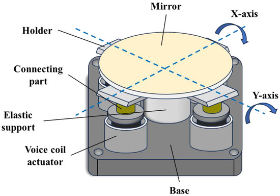
Figure 2.
Structure of a two-axis tip–tilt mirror.
We therefore model the TTM system as follows:
where and represent the natural frequency and damping factor of the TTM, respectively.
For the external reference signal, a sinusoidal signal with an amplitude of 5 urad is generated using model (3), and its system matrix can be expressed as
where . is the center frequency of the sinusoidal signal and is the system’s sampling rate. The entire control block diagram of applying the proposed noisy-OPFB Q-learning algorithm to the TTM tracking control system is shown in Figure 3. It should be emphasized that all the data used throughout the operation and optimization of the TTM tracking control system include only the control input and the noisy tracking error and do not depend on any of the system state information. This highlights the advantages of our proposed method over other Q-learning based methods.
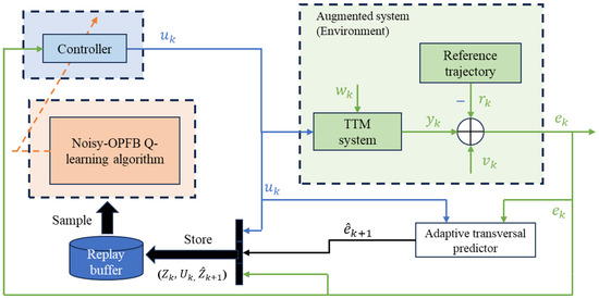
Figure 3.
The noisy-OPFB Q-learning tracking control scheme with application to a TTM system.
For simulation purposes, we consider only one axis of the TTM, and the sampling rate was set to 1 KHz. The parameters of the TTM are the same as those identified in [39]: and . The cost function remains in the form of (18), where we let , , and . The lengths of data history used for state estimation and output prediction were selected by and then . Thus, there are a total of 528 unknown parameters to be learned in the kernel matrix H and 31 unknown parameters to be learned in the controller. The rank condition is satisfied by adding an exploration noise with zero mean and unit variance ; the batch size is chosen as l = 600. In the subsequent simulations, we set the size of the experience replay buffer to 1000, which means that the system requires a 1 s sampling period to obtain a sufficient amount of training data, and these 1000 sets of data constitute the entire dataset needed for training. The initial controller gain was selected as .
4.2. Convergency Analysis
The convergence performance of the proposed algorithm is first verified. The process noise and measurement noise are assumed to be Gaussian white noise with distribution and . Considering a 10 Hz reference jitter signal and running the TTM control system shown in Figure 3 for 3 s, the tracking control trajectory is shown in Figure 4. It is observed that the controller converges after 1.75 s of learning, and the convergence curves of the controller parameters are displayed in Figure 5. The results show that the controller converges after only seven iterations, which is due to the fact that the proposed noisy-OPFB Q-learning algorithm is updated through efficient numerical solutions rather than stochastic gradient methods, ensuring a rapid and stable convergence process for the controller parameters. To further demonstrate that the trained controller is near optimal, we executed the algorithm 20 times under stochastic noise conditions and compared all solutions with the optimal analytical solution, as shown in Figure 6. The root-mean-square error (RMSE) between the near optimal solutions and the optimal analytical solution is only 0.027. This indicates that despite the introduction of approximation errors and random noise interference during the computation process, the proposed algorithm can still converge well near the optimal solution.
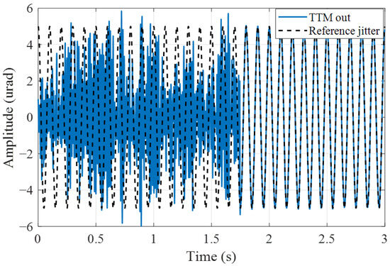
Figure 4.
Jitter tracking control trajectory of the TTM system.
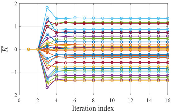
Figure 5.
Convergence curve of the controller. Each line corresponds to a parameter of the controller.
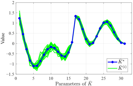
Figure 6.
Comparison of the solutions of 20 experiments with the optimal analytical solution. The green line indicates the solution in each experiment and the blue line indicates the optimal solution .
4.3. Tracking Control Performance Analysis
Considering the proposed algorithm directly optimizes the controller using noisy measurements, it is essential to analyze the impact of different camera detection noise levels on the jitter tracking performance. Figure 7, Figure 8 and Figure 9 illustrate the tracking effects on a 10 Hz reference jitter signal under measurement noise standard deviation (STD) of 0, 0.5, and 1. The results show that almost complete suppression of jitter is achieved in the absence of noise, while the jitter suppression effect deteriorates with increasing measurement noise STD. Figure 10 presents how the jitter tracking RMSEvaries with the noise STD. It can be observed that there is a roughly linear relationship between the noise STD and tracking RMSE, indicating that the noise level is directly related to tracking performance, and the estimation error introduced by noise is the primary factor affecting Algorithm 3. Nonetheless, fluctuations in the intensity of measurement noise over a wide range do not have a major impact on the tracking effectiveness and stability of the controller. This suggests that our proposed algorithm can accurately deduce the system’s dynamic characteristics from noisy measurements, thereby correctly calculating a near-optimal tracking controller. It eliminates the need for assumptions about measurable state information and the design of state observers, and thus is more generalizable and practical.
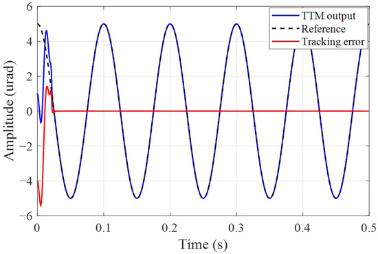
Figure 7.
Jitter tracking error with noise STD .
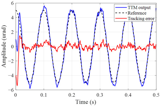
Figure 8.
Jitter tracking error with noise STD .
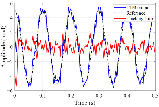
Figure 9.
Jitter tracking error with noise STD .
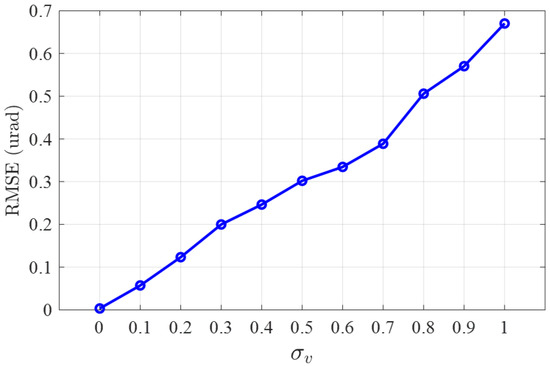
Figure 10.
Tracking RMSE at different measurement noise STD .
Furthermore, we verified the tracking control effectiveness of the proposed algorithm for beam jitter signals of different frequencies with measurement noise STD . The jitter tracking RMSE of the proposed algorithm was compared with that of a traditional integral controller, with the results presented in Table 1. From the results, it can be seen that with the increase in the jitter frequency, the integrator, limited by its control bandwidth, struggles to maintain tracking performance. Meanwhile, the phase lag effect causes an amplification of the jitter signal at 30 Hz, leading to a decrease in system stability. In contrast, the proposed algorithm achieved precise and stable tracking for both low and high frequencies; the RMSE is reduced up to 98.7%. Figure 11 shows a comparison example of the tracking error of a 100 Hz reference jitter. From the comparison results of power spectral density (PSD), the tracking error of the proposed method at 100 Hz is only −30 dB, which is 40.5 dB lower compared to the error of integral control. Therefore, in contrast to the traditional integrator, the noisy-OPFB Q-learning is independent of control bandwidth and can autonomously tailor the controller to various reference jitter signals, thus achieving broadband jitter tracking. This comparison underscores the effectiveness and adaptability of the proposed algorithm when applied to tilting mirror systems, making it a potent solution for beam jitter control issues.

Table 1.
Beam jitter tracking RMSE (urad) of different control methods.
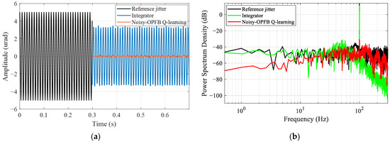
Figure 11.
Tracking comparison of different controllers under 100 Hz reference jitter: (a) RMSE; (b) power spectral density.
Finally, the algorithm’s adaptability to time-varying reference jitter signals and system models was analyzed, and the corresponding tracking trajectory is shown in Figure 12. To simulate environmental and reference signal changes, the frequency of the external jitter signal was changed from the initial 6 Hz to 13 Hz at 3 s. At the same time, the natural resonance frequency and the damping coefficient of the TTM model are changed to and , respectively. The trajectory in Figure 12 indicates that after a period of adaptation and learning, the controller can once again accurately track the jitter signal. The learning curve of the controller parameters in Figure 13 demonstrates that Algorithm 3 can continue to learn on the basis of an existing controller without the need for an additional parameter tuning process. It should be noted that the whole trajectory is closed-loop continuous, and the proposed algorithm does not cause any degradation of system stability during the updating process. This illustrates that the proposed algorithm possesses online learning and adaptive capabilities and could effectively address the tracking control issues of dynamic beam jitter in the TTM system caused by environmental changes.
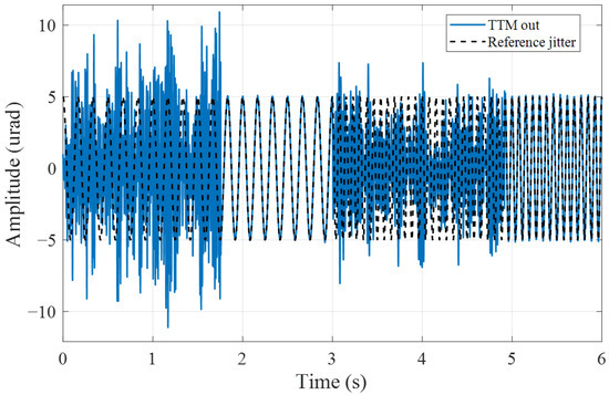
Figure 12.
Tracking control trajectory under time-varying reference jitter.
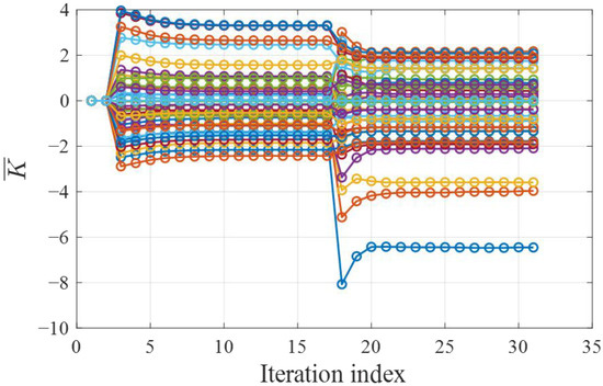
Figure 13.
Convergence curves of controller under time-varying reference jitter. Each line corresponds to a parameter of the controller.
5. Conclusions
This paper develops a noisy-OPFB Q-learning scheme to address the optimal tracking control problem for TTM systems under conditions of additive unknown noise interference, unmeasurable system states, and unknown system dynamics. This method adjusts the Bellman equation through the estimation theory and employs an adaptive transversal predictor and experience replay technique, which is able to obtain a fast and stable near-optimal solution in spite of interference from stochastic noise. The numerical iterative computation process based on Q-learning releases the reliance on neural network design, thus facilitating easier deployment in practical systems. We have applied the algorithm to an application example of a TTM tracking control simulation system, demonstrating the effectiveness of the proposed method. Compared to traditional integral control, our reinforcement learning-based approach exhibits better control stability, dynamic adaptability, and tracking performance. This offers the potential for realizing intelligent control of optical systems. Our future work will focus on deploying the scheme in actual systems and finding better methods to reduce the computational costs of complex systems.
Author Contributions
Conceptualization, S.G. and T.C.; methodology, S.G.; investigation, S.G. and Z.G.; data curation, S.G.; writing—original draft preparation, S.G.; writing—review and editing, T.C., Z.G., and P.Y.; visualization, Z.G. and L.K.; supervision, S.W. and P.Y.; resources, S.W. and P.Y. All authors have read and agreed to the published version of the manuscript.
Funding
This research was funded by the National Natural Science Foundation of China (No. 62005285, No. 62105336, No. 62305343).
Institutional Review Board Statement
Not applicable.
Informed Consent Statement
Not applicable.
Data Availability Statement
The data presented in this study are available on request from the corresponding author.
Conflicts of Interest
The authors declare no conflicts of interest.
References
- Arikawa, M.; Ito, T. Performance of Mode Diversity Reception of a Polarization-Division-Multiplexed Signal for Free-Space Optical Communication under Atmospheric Turbulence. Opt. Express 2018, 26, 28263. [Google Scholar] [CrossRef] [PubMed]
- Clénet, Y.; Kasper, M.; Ageorges, N.; Lidman, C.; Fusco, T.; Marco, O.P.; Hartung, M.; Mouillet, D.; Koehler, B.; Rousset, G. NAOS Performances: Impact of the Telescope Vibrations and Possible Origins. In Proceedings of the SF2A-2004: Semaine de l’Astrophysique Francaise, Paris, France, 14–18 June 2004; p. 179. [Google Scholar]
- Maly, J.R.; Erickson, D.; Pargett, T.J. Vibration Suppression for the Gemini Planet Imager. In Proceedings of the Ground-Based and Airborne Telescopes III, San Diego, CA, USA, 27 June–2 July 2010; SPIE: Bellingham, WA, USA, 2010; Volume 7733, pp. 506–514. [Google Scholar]
- Nousiainen, J.; Rajani, C.; Kasper, M.; Helin, T.; Haffert, S.Y.; Vérinaud, C.; Males, J.R.; Van Gorkom, K.; Close, L.M.; Long, J.D.; et al. Towards On-Sky Adaptive Optics Control Using Reinforcement Learning. A&A 2022, 664, A71. [Google Scholar] [CrossRef]
- Pou, B.; Ferreira, F.; Quinones, E.; Gratadour, D.; Martin, M. Adaptive Optics Control with Multi-Agent Model-Free Reinforcement Learning. Opt. Express 2022, 30, 2991. [Google Scholar] [CrossRef] [PubMed]
- Ke, H.; Xu, B.; Xu, Z.; Wen, L.; Yang, P.; Wang, S.; Dong, L. Self-Learning Control for Wavefront Sensorless Adaptive Optics System through Deep Reinforcement Learning. Optik 2019, 178, 785–793. [Google Scholar] [CrossRef]
- Landman, R.; Haffert, S.Y.; Radhakrishnan, V.M.; Keller, C.U. Self-Optimizing Adaptive Optics Control with Reinforcement Learning for High-Contrast Imaging. J. Astron. Telesc. Instrum. Syst. 2021, 7, 039002. [Google Scholar] [CrossRef]
- Werbos, P. Approximate Dynamic Programming for Real-Time Control and Neural Modeling. In Handbook of Intelligent Control; Van Nostrand Reinhold: New York, NY, USA, 1992. [Google Scholar]
- Qasem, O.; Gao, W. Robust Policy Iteration of Uncertain Interconnected Systems with Imperfect Data. IEEE Trans. Automat. Sci. Eng. 2023, 21, 1214–1222. [Google Scholar] [CrossRef]
- Song, R.; Lewis, F.L. Robust Optimal Control for a Class of Nonlinear Systems with Unknown Disturbances Based on Disturbance Observer and Policy Iteration. Neurocomputing 2020, 390, 185–195. [Google Scholar] [CrossRef]
- Al-Tamimi, A.; Lewis, F.L.; Abu-Khalaf, M. Model-Free Q-Learning Designs for Linear Discrete-Time Zero-Sum Games with Application to H-Infinity Control. Automatica 2007, 43, 473–481. [Google Scholar] [CrossRef]
- Li, Z.; Wang, M.; Ma, G. Adaptive Optimal Trajectory Tracking Control of AUVs Based on Reinforcement Learning. ISA Trans. 2023, 137, 122–132. [Google Scholar] [CrossRef]
- Wang, N.; Gao, Y.; Zhang, X. Data-Driven Performance-Prescribed Reinforcement Learning Control of an Unmanned Surface Vehicle. IEEE Trans. Neural Netw. Learning Syst. 2021, 32, 5456–5467. [Google Scholar] [CrossRef]
- Rizvi, S.A.A.; Pertzborn, A.J.; Lin, Z. Reinforcement Learning Based Optimal Tracking Control Under Unmeasurable Disturbances With Application to HVAC Systems. IEEE Trans. Neural Netw. Learn. Syst. 2022, 33, 7523–7533. [Google Scholar] [CrossRef] [PubMed]
- Wang, R.; Ma, D.; Li, M.-J.; Sun, Q.; Zhang, H.; Wang, P. Accurate Current Sharing and Voltage Regulation in Hybrid Wind/Solar Systems: An Adaptive Dynamic Programming Approach. IEEE Trans. Consumer Electron. 2022, 68, 261–272. [Google Scholar] [CrossRef]
- Yang, J.; Wang, Y.; Wang, T.; Yu, X. Optimal Tracking Control For A Two-Link Robotic Manipulator Via Adaptive Dynamic Programming. In Proceedings of the 2020 Chinese Automation Congress (CAC), Shanghai, China, 6 November 2020; pp. 2687–2692. [Google Scholar]
- Fang, H.; Zhu, Y.; Dian, S.; Xiang, G.; Guo, R.; Li, S. Robust Tracking Control for Magnetic Wheeled Mobile Robots Using Adaptive Dynamic Programming. ISA Trans. 2022, 128, 123–132. [Google Scholar] [CrossRef] [PubMed]
- Littman, M.L. A Tutorial on Partially Observable Markov Decision Processes. J. Math. Psychol. 2009, 53, 119–125. [Google Scholar] [CrossRef]
- Liu, D.; Huang, Y.; Wang, D.; Wei, Q. Neural-Network-Observer-Based Optimal Control for Unknown Nonlinear Systems Using Adaptive Dynamic Programming. Int. J. Control. 2013, 86, 1554–1566. [Google Scholar] [CrossRef]
- Mu, C.; Wang, D.; He, H. Novel Iterative Neural Dynamic Programming for Data-Based Approximate Optimal Control Design. Automatica 2017, 81, 240–252. [Google Scholar] [CrossRef]
- Zhang, H.; Cui, L.; Zhang, X.; Luo, Y. Data-Driven Robust Approximate Optimal Tracking Control for Unknown General Nonlinear Systems Using Adaptive Dynamic Programming Method. IEEE Trans. Neural Netw. 2011, 22, 2226–2236. [Google Scholar] [CrossRef] [PubMed]
- Rizvi, S.A.A.; Lin, Z. Output Feedback Q-Learning Control for the Discrete-Time Linear Quadratic Regulator Problem. IEEE Trans. Neural Netw. Learn. Syst. 2019, 30, 1523–1536. [Google Scholar] [CrossRef]
- Liu, Y.; Zhang, H.; Yu, R.; Qu, Q. Data-Driven Optimal Tracking Control for Discrete-Time Systems with Delays Using Adaptive Dynamic Programming. J. Frankl. Inst. 2018, 355, 5649–5666. [Google Scholar] [CrossRef]
- Kiumarsi, B.; Lewis, F.L.; Naghibi-Sistani, M.-B.; Karimpour, A. Optimal Tracking Control of Unknown Discrete-Time Linear Systems Using Input-Output Measured Data. IEEE Trans. Cybern. 2015, 45, 2770–2779. [Google Scholar] [CrossRef]
- Wang, T.; Zhang, H.; Luo, Y. Stochastic Linear Quadratic Optimal Control for Model-Free Discrete-Time Systems Based on Q-Learning Algorithm. Neurocomputing 2018, 312, 1–8. [Google Scholar] [CrossRef]
- Pang, B.; Jiang, Z.-P. Robust Reinforcement Learning: A Case Study in Linear Quadratic Regulation. AAAI 2021, 35, 9303–9311. [Google Scholar] [CrossRef]
- Tao, B.; Zhong-Ping, J. Adaptive Optimal Control for Linear Stochastic Systems with Additive Noise. In Proceedings of the 2015 34th Chinese Control Conference (CCC), Hangzhou, China, 28–30 July 2015; pp. 3011–3016. [Google Scholar]
- Lai, J.; Xiong, J.; Shu, Z. Model-Free Optimal Control of Discrete-Time Systems with Additive and Multiplicative Noises. Automatica 2023, 147, 110685. [Google Scholar] [CrossRef]
- Zhang, M.; Gan, M.-G.; Chen, J. Data-Driven Adaptive Optimal Control for Stochastic Systems with Unmeasurable State. Neurocomputing 2020, 397, 1–10. [Google Scholar] [CrossRef]
- Kiumarsi, B.; Lewis, F.L.; Modares, H.; Karimpour, A.; Naghibi-Sistani, M.-B. Reinforcement-Learning for Optimal Tracking Control of Linear Discrete-Time Systems with Unknown Dynamics. Automatica 2014, 50, 1167–1175. [Google Scholar] [CrossRef]
- Lancaster, P.; Rodman, L. Algebraic Riccati Equations, Clarendon Press: Oxford, UK, 1995; ISBN 0-19-159125-4.
- Speyer, J.L.; Chung, W.H. Stochastic Processes, Estimation, and Control, 1st ed.; Advances in Design and Control; Society for Industrial and Applied Mathematics: Philadelphia, PA, USA, 2008; ISBN 978-0-89871-655-9. [Google Scholar]
- Chen, C.-W.; Huang, J.-K. Adaptive State Estimation for Control of Flexible Structures. In Proceedings of the Advances in Optical Structure Systems, Orlando, FL, USA, 16–20 April 1990; Breakwell, J.A., Genberg, V.L., Krumweide, G.C., Eds.; SPIE: Bellingham, WA, USA, 1990; p. 252. [Google Scholar]
- Lewis, F.L.; Vrabie, D.; Vamvoudakis, K.G. Reinforcement Learning and Feedback Control: Using Natural Decision Methods to Design Optimal Adaptive Controllers. IEEE Control Syst. 2012, 32, 76–105. [Google Scholar] [CrossRef]
- Malla, N.; Ni, Z. A New History Experience Replay Design for Model-Free Adaptive Dynamic Programming. Neurocomputing 2017, 266, 141–149. [Google Scholar] [CrossRef]
- Song, R.; Lewis, F.L.; Wei, Q.; Zhang, H. Off-Policy Actor-Critic Structure for Optimal Control of Unknown Systems with Disturbances. IEEE Trans. Cybern. 2016, 46, 1041–1050. [Google Scholar] [CrossRef] [PubMed]
- Bian, T.; Jiang, Y.; Jiang, Z.-P. Adaptive Dynamic Programming for Stochastic Systems with State and Control Dependent Noise. IEEE Trans. Autom. Control. 2016, 61, 4170–4175. [Google Scholar] [CrossRef]
- Li, M.; Qin, J.; Zheng, W.X.; Wang, Y.; Kang, Y. Model-Free Design of Stochastic LQR Controller from Reinforcement Learning and Primal-Dual Optimization Perspective. arXiv 2021, arXiv:2103.09407. [Google Scholar]
- Lu, Y.; Fan, D.; Zhang, Z. Theoretical and Experimental Determination of Bandwidth for a Two-Axis Fast Steering Mirror. Optik 2013, 124, 2443–2449. [Google Scholar] [CrossRef]
Disclaimer/Publisher’s Note: The statements, opinions and data contained in all publications are solely those of the individual author(s) and contributor(s) and not of MDPI and/or the editor(s). MDPI and/or the editor(s) disclaim responsibility for any injury to people or property resulting from any ideas, methods, instructions or products referred to in the content. |
© 2024 by the authors. Licensee MDPI, Basel, Switzerland. This article is an open access article distributed under the terms and conditions of the Creative Commons Attribution (CC BY) license (https://creativecommons.org/licenses/by/4.0/).