Article

Cross-Correlation Algorithm Based on Speeded-Up Robust Features Parallel Acceleration for Shack–Hartmann Wavefront Sensing

1
National Laboratory on Adaptive Optics, Chengdu 610209, China
2
Institute of Optics and Electronics, Chinese Academy of Sciences, Chengdu 610209, China
3
School of Optoelectronics, University of Chinese Academy of Sciences, Beijing 100049, China
4
School of Electronic, Electrical and Communication Engineering, University of Chinese Academy of Sciences, Beijing 100049, China
*
Author to whom correspondence should be addressed.
Photonics 2024, 11(9), 844; https://doi.org/10.3390/photonics11090844
Submission received: 23 July 2024 / Revised: 20 August 2024 / Accepted: 1 September 2024 / Published: 5 September 2024
(This article belongs to the Special Issue Challenges and Future Directions in Adaptive Optics Technology)

Abstract

:
A cross-correlation algorithm to obtain the sub-aperture shifts that occur is a crucial aspect of scene-based SHWS (Shack–Hartmann wavefront sensing). However, when the sub-image is partially absent within the atmosphere, the traditional cross-correlation algorithm can easily obtain the wrong shift results. To overcome this drawback, we propose an algorithm based on SURFs (speeded-up-robust features) matching. In addition, to meet the speed required by wavefront sensing, CUDA parallel optimization of SURF matching is carried out using a GPU thread execution model and a programming model. The results show that the shift error can be reduced by more than two times, and the parallel algorithm can achieve nearly ten times the acceleration ratio.

1. Introduction

Wavefront sensing is a key aspect of the Adaptive Optics (AOs) technique that is extensively used in many areas, including large aperture astronomical telescopes, short-range laser transmission and optical microscopy [1,2,3,4,5]. Due to the advantages of a simple geometric structure, high processing speed and light energy utilization, the Shack–Hartmann wavefront sensor has become a popular wavefront sensing instrument. When the object is an extended scene, and not a point source, the Hartmann sub-apertures form images of the observed scene. The light field distribution of the sub-image of the Hartmann wavefront sensor is equal to the convolution of the ideal geometric optical image and the system point spread function, and the microlens array of the Hartmann wavefront sensor divides the incident distorted wavefront so that the sub-wavefront corresponding to the microlens can be approximately considered to contain only tilt. In this case, the procedure by which the shifts between the sub-images occurs is usually measured by cross-correlation analysis. Firstly, the image with the best quality is selected as the reference image, and then the shift results are obtained by matching the other sub-images with the reference image.
There are many fields of application for scene-based SHWS, such as imaging conducted along horizontal paths through the atmosphere [6], earth-observation satellites [7] and observations of the sun during the daytime [8]. Poyneer found that the cross-correlation algorithm works well in these applications in terms of both its performance with noise and its computational simplicity [9]. In this approach, the shifts between the reference image and other sub-images are determined from the location of their cross-correlation peaks.
So far, many analyses and improvements have been proposed for the cross-correlation approach. Hu Xinqi et al. [10] described the sub-image structure with a spatial spectrum and systematically analyzed the influence of sub-image structure and noise on the precision of scene-based SHWS. Erkin et al. [11] proposed the adaptive periodic-correlation (APC) algorithm to obtain a high precision, and [12] found that the error component depends on the content of the extended scene, and subtracting this component can improve APC. Wang Yawen et al. [13] proposed a Gamma-correlation algorithm and gradient cross-correlation algorithm to solve the problem of low sub-image contrast and the wraparound effect. Despite all of these improvements, the cross-correlation method still has a serious problem: the phenomenon of the partial absence of sub-images. Because the real-time motion change frequency of the object scene is greater than the Shack–Hartmann sensor sampling frequency, the sub-image is prone to partial absence, and this is common both at the short-range kilometer level or in tilted laser transmission, even when there is little content within the sub-images.
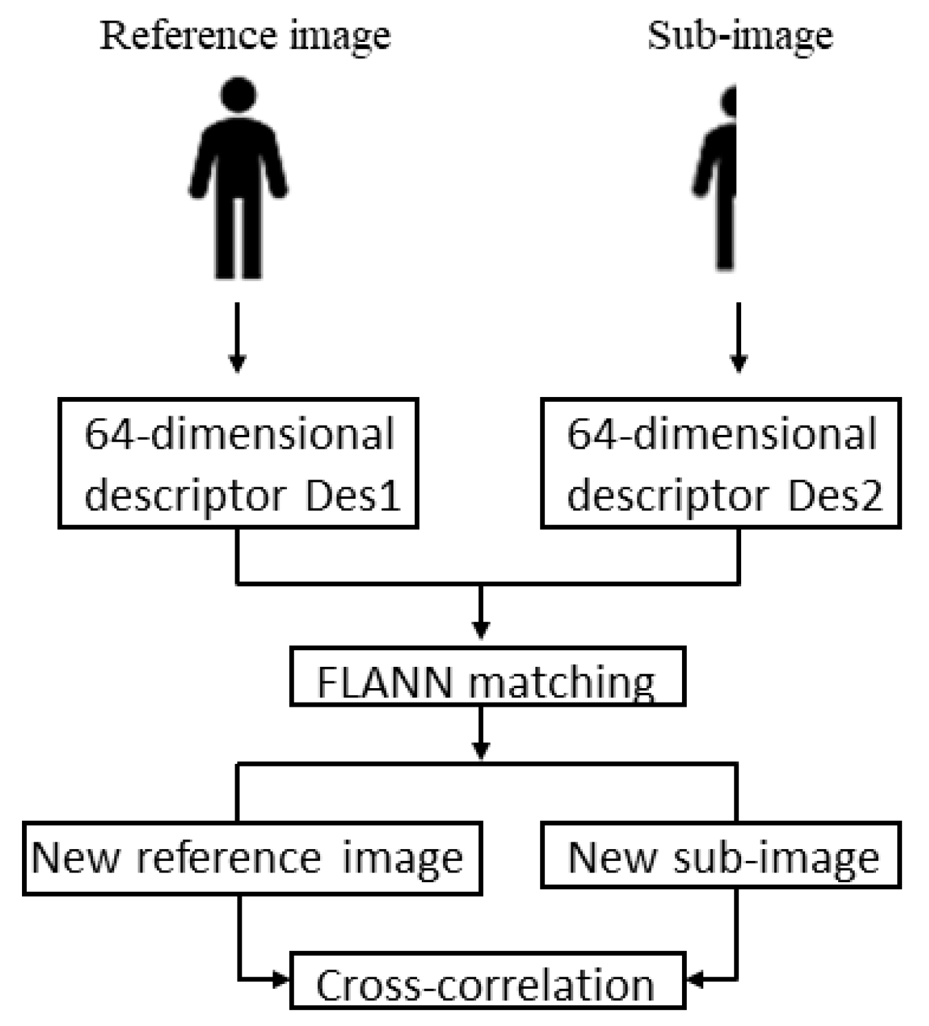
To address the above issue, this paper proposes a SURF-matching parallel acceleration method. In our method, after the Shack–Hartmann sensor acquires the sub-images, the reference image and each sub-image are first analyzed to detect, describe and match them using the SURF matching method. CUDA parallel optimization was carried out for SURF feature detection and description. Next, the matching pairs of each sub-image and reference image were retained as new images for the cross-correlation analysis. The digital simulation shows that the method can effectively minimize the effect of partially absent sub-images on wavefront sensing and quickly obtain shift results compared to the classical SURF matching method.

2. Principles and Methods

2.1. The Cross-Correlation Algorithm Description

We considered two sub-images formed by the two distinct sub-apertures of the scene-based SHWS (they are both N × N pixels), and the center of the sub-image with the best quality in the Shack–Hartmann array was used as the reference image I r x , y (it was M × M pixels including the object scene content, M < N); the other image was the test sub-image I a α + x , + y , where the α and are not necessarily integer amounts. As shown in Figure 1, the two finite pixel images traverse from left to right and from top to bottom. The normalized cross-correlation algorithm is expressed as follows [14]:
S ( α ,   ) = x = 1 M y = 1 M I r x , y - I r x , y ¯ × I a α + x , + y - I a α + x , + y ¯ x = 1 M y = 1 M I r x , y - I r x , y ¯ 2 × x = 1 M y = 1 M I a α + x , + y - I a α + x , + y ¯ 2 ,  
The denominator part of the formula is used for normalization. The I r x , y ¯ and I a α + x , + y ¯ represent the average gray values of the reference image pixels and the test sub-image pixels.
If we assume that the integer location of the maximum S ( α ,   ) is at ( Δ x , Δ y ) , then the sub-pixel estimation of the shift α can be obtained by parabolic interpolation [15]:
α = Δ x + 0.5 [ s ( Δ x 1 , Δ y ) s ( Δ x + 1 , Δ y ) ] s ( Δ x 1 , Δ y ) + s ( Δ x + 1 , Δ y ) 2 s ( Δ x , Δ y ) ,  

2.2. SURF Matching Parallel Acceleration Processing Analysis

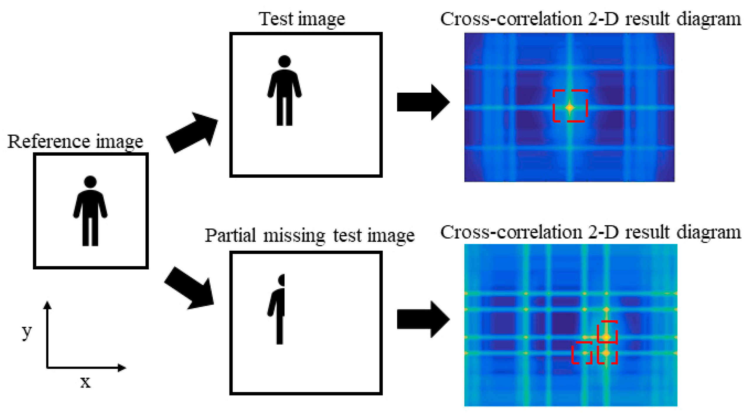
When the reference image of the M × M part is moved onto the test sub-image, the test sub-image shows a partial absence phenomenon. As shown in Figure 2, the object scene is a human icon, and multiple cross-correlation peaks appear (shown in the red boxes in Figure 2), which directly obtain the wrong shift results.
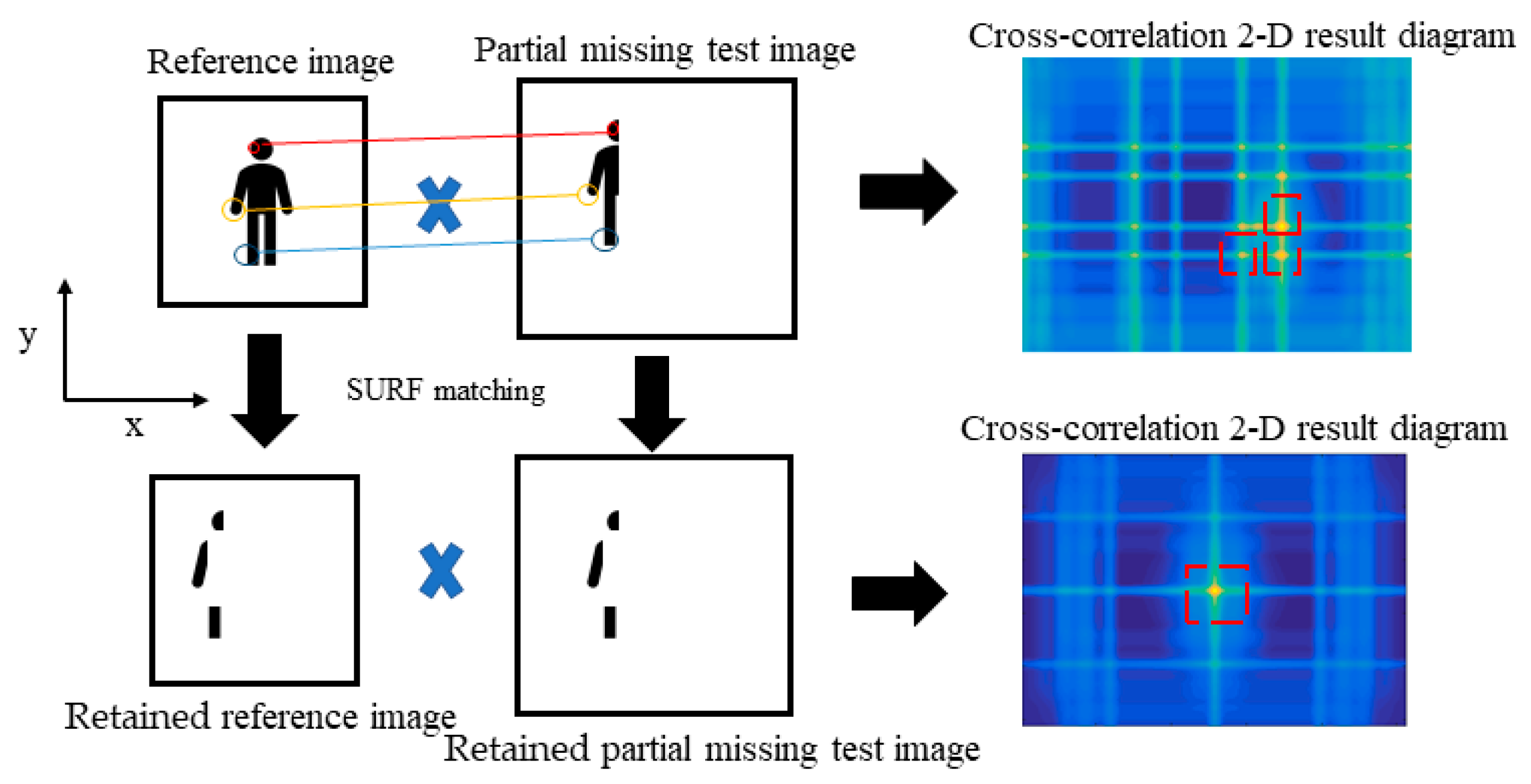
The partial absence test sub-image and the reference image pairs are matched by SURF, and only the matching pairs are retained before the subsequent cross-correlation analysis. As shown in Figure 3.
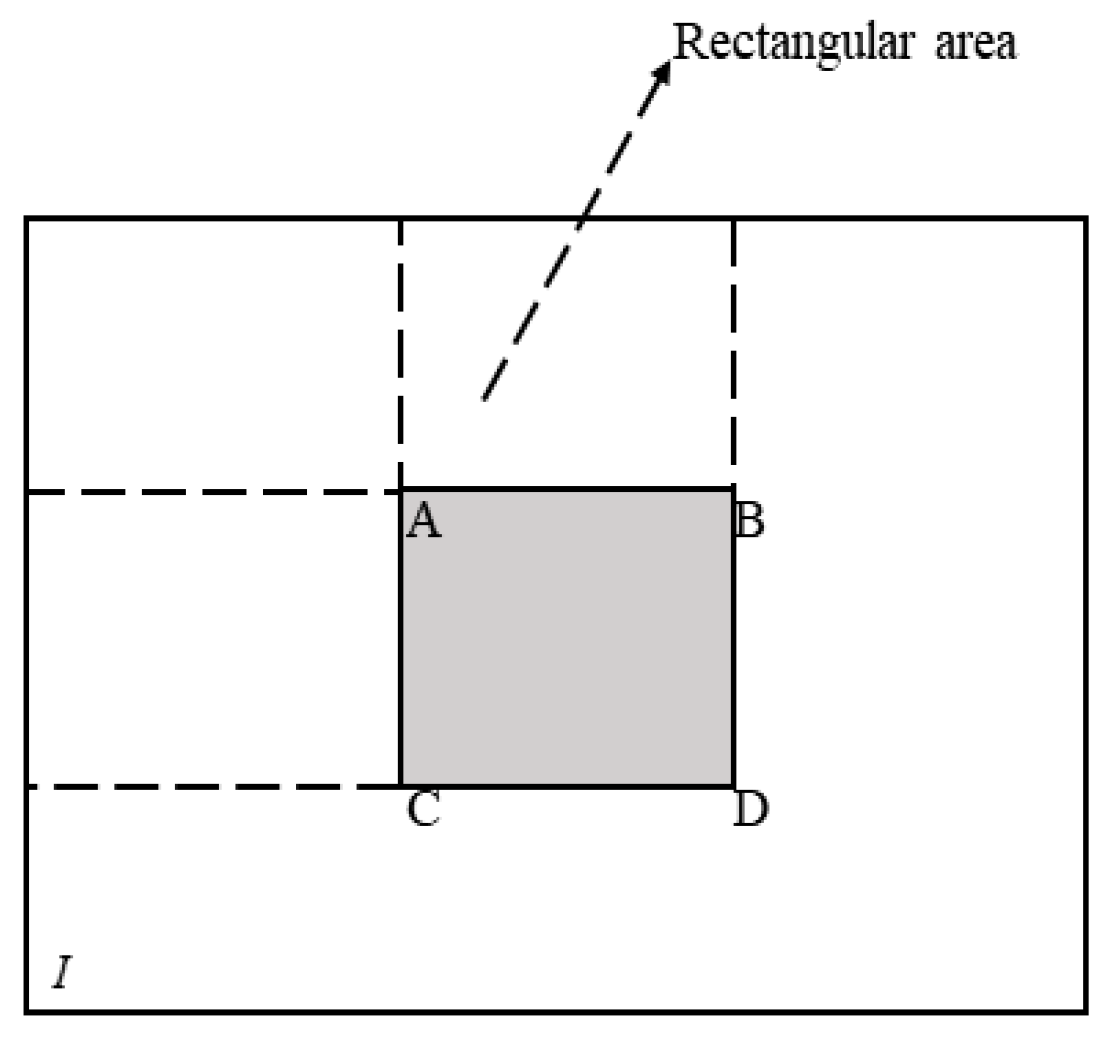
Any sub-images obtained by Shack-Hartmann are converted into a grayscale image. As shown in Equation (4), SURF matching first needs to define the integral image I Σ ( x ) of a gray image I at any pixel point X ( x , y ) as the sum of the gray values of all pixels in the rectangular area composed of the original point and X in the input image I . As shown in Figure 4, the integral image of any rectangular area ABCD is a simple sum of the integral images of each vertex area: [16].
I Σ ( X ) = i = 0 x j = 0 y I ( i , j ) ,
I Σ A B C D = I Σ A + I Σ D I Σ B I Σ C ,
The Hessian matrix of pixel X ( x , y ) at scale σ on image I Σ ( x ) is defined as:
H ( x , σ ) = [ L x x ( X , σ ) L x y ( X , σ ) L x y ( X , σ ) L y y ( X , σ ) ] ,
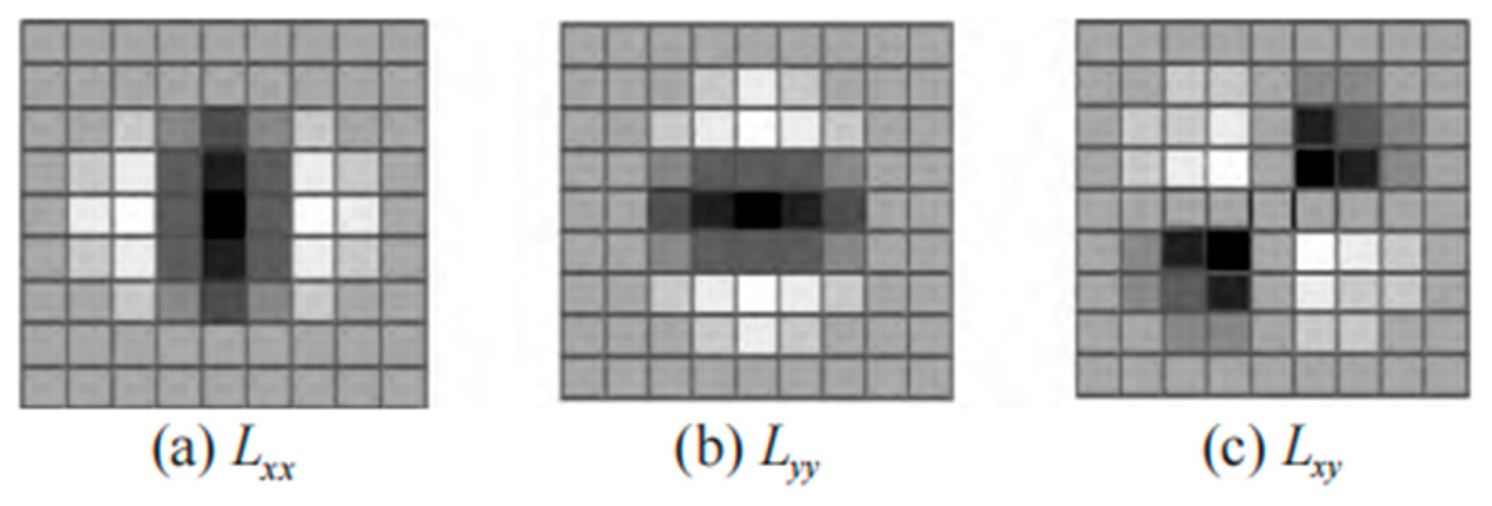
Here, L x x ( X , σ ) is the convolution of image I Σ ( x ) and the second-order partial derivative of the Gaussian 2 x 2 g ( σ ) , L x y ( X , σ ) and L y y ( X , σ ) are similar.
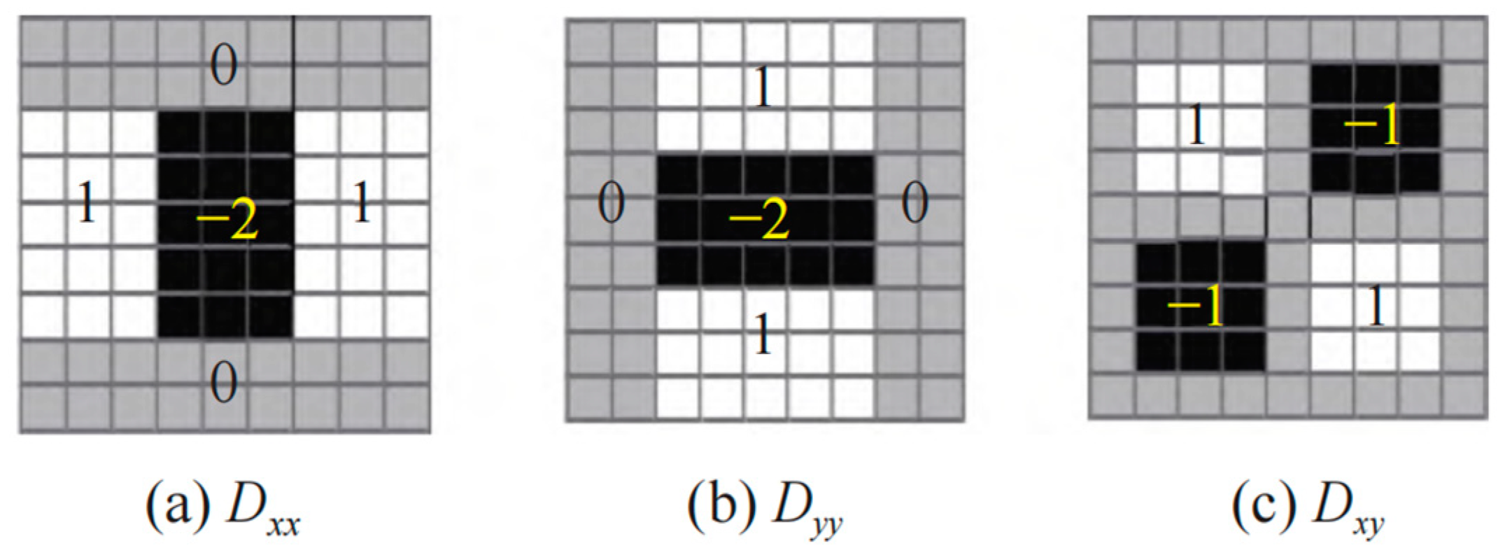
As shown in Figure 5, the SURF matching uses box filters with different weights for two-dimensional Gaussian filtering to approximate the second-order Gaussian partial derivative. This process can reduce the computational cost by using the integral image [17].
The 9 × 9 box filter in Figure 6 is the Gaussian approximation of scale σ = 1.2, which represents the highest spatial resolution and is represented by D x x , D y y and D x y , respectively. Then, the Hessian matrix discriminant (DOH value) is defined as [18]:
d e t ( H ) = D x x D y y ( c D x y ) 2 ,
The weight coefficient c takes the empirical value of 0.9.
The SURF matching constructs the scale space by increasing the size of the box filter. The SURF scale space is divided into several octaves. In Figure 6, the 9 × 9 box filter is the first octave of the SURF scale space, which is used to calculate the minimum scale Hessian response value ( σ 0 = 1.2). The sampling interval of each octave is doubled, and the size of the box filter of the adjacent octave is increased by 6 pixels steps. The SURF scale space template size can be obtained from Equation (7) [19]:
L = 3 × 2 o c t a v e × i n t e r v a l + 1 ,
The corresponding scales of different octaves are:
s = σ 0 × L 9 = 1.2 × L 9 ,
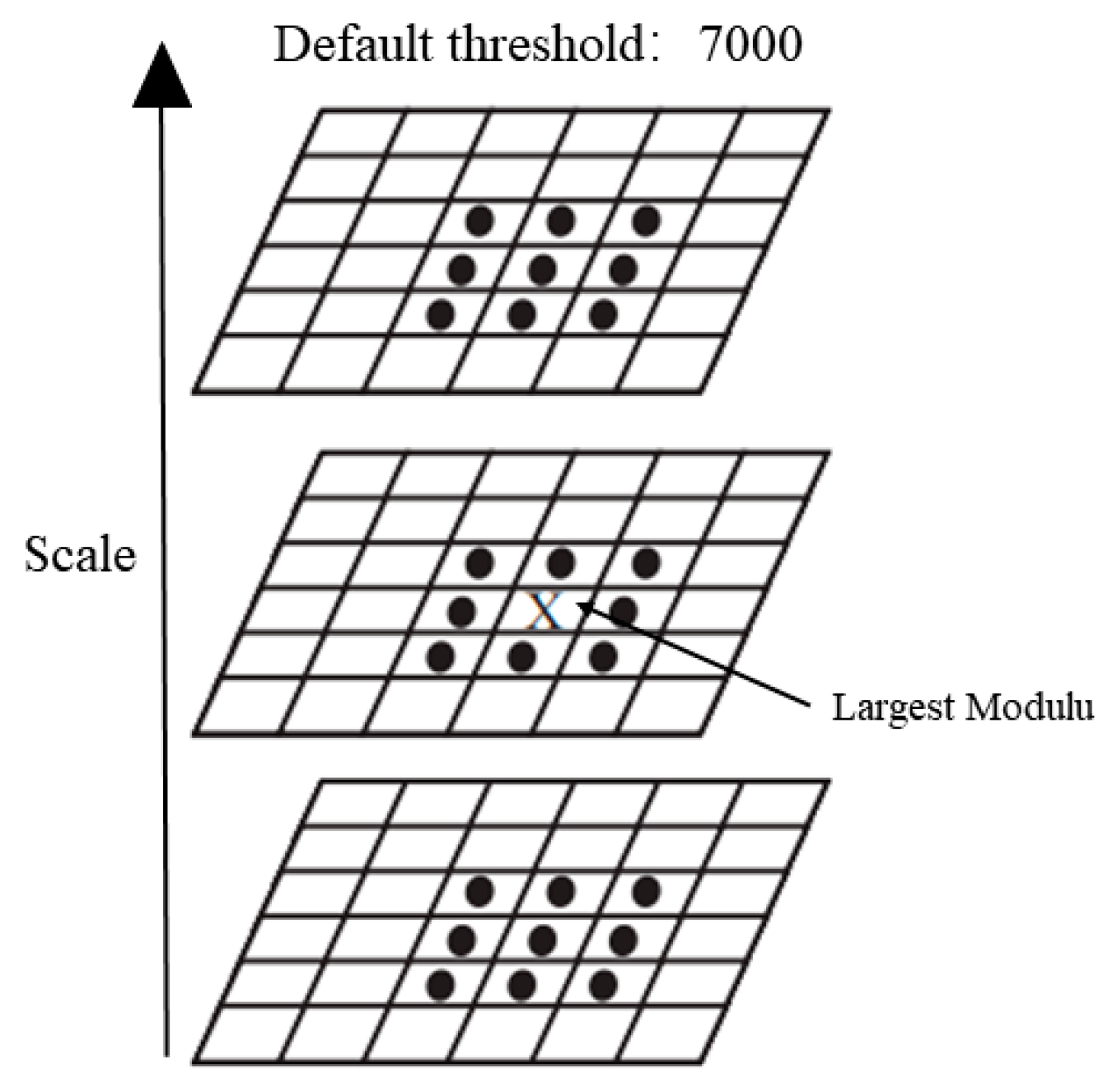
The SURF matching uses 3 × 3 × 3 neighborhood non-maximum suppression to detect feature points. As shown in Figure 7, the DOH value of each pixel calculated by Equation (7) is compared with 26 points in its 3 × 3 × 3 neighborhood. If the modulus of the point is the largest, it is initially set as the extreme point. Then, the unstable and weak interest points are removed, and the points whose values are greater than the threshold are selected as the final feature points [19].
After the above detection task is completed, the feature points need to be described. Firstly, the main direction of feature points is determined. In order to ensure the rotation invariance of the image, the SURF determines the main direction of each feature point by calculating the Haar wavelet response in the neighborhood of the feature point.
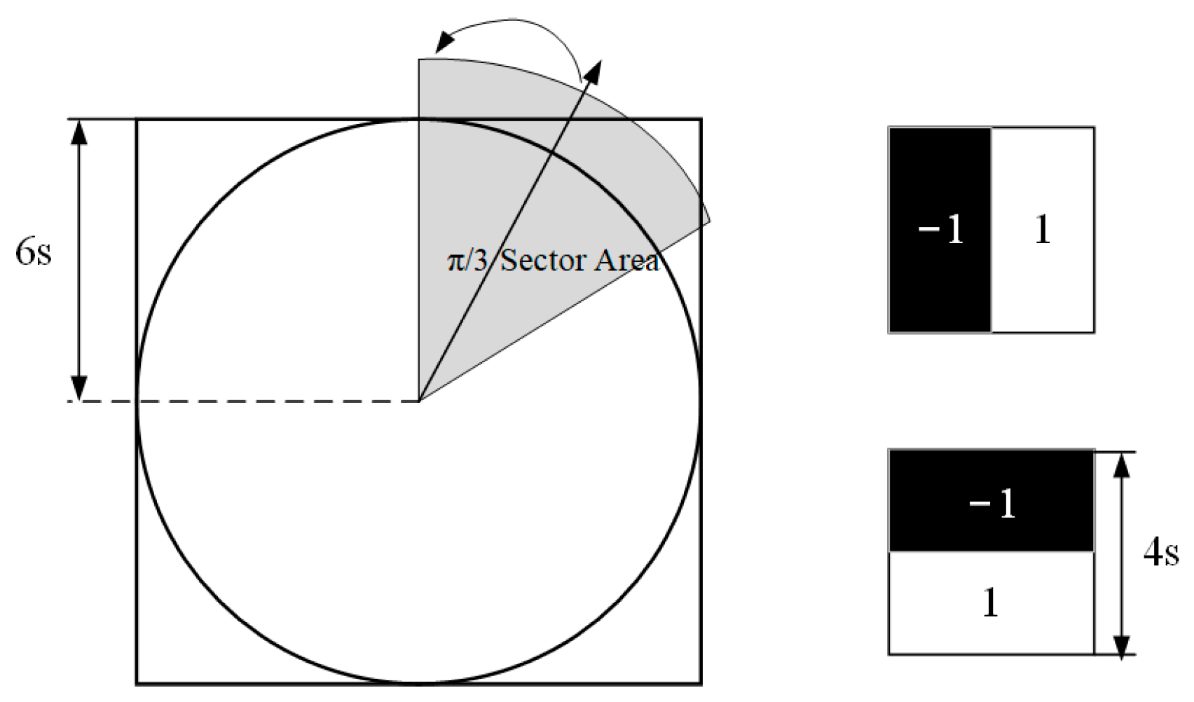
As shown in Figure 8, taking the feature point as the center, a Haar wavelet template with the size of 4 s was used to calculate the wavelet response d x and d y in the x and y directions in the circular neighborhood with a radius of 6 s . The sum of the horizontal and vertical responses of all feature points in the sector sliding window sliding along the counterclockwise direction was calculated, and a local direction vector ( m ω , θ ω ) was obtained. The longest vector in all windows was defined as the main direction of the feature points [19]:
m ω = ω d x + ω d y
θ ω = arctan ω d x ω d y
θ = θ ω max m ω
We then regenerated the feature point descriptors. Taking the feature point as the center and the main direction of the feature point as the x-axis, a square region with a side length of 20 s was constructed, and it was equally divided into 4 × 4 square sub-regions with a side length of 5 s . The Haar wavelet response with a template size of 2 s in each sub-region was calculated to obtain a 4-dimensional feature descriptor vector:
V = ( d x , d x , d x , d y )
Here, d x and d y are Haar wavelet responses in x and y directions. In this way, the 64-dimensional descriptor of the feature point can be obtained in 16 sub-regions.
The SURF matching uses the Euclidean distance to characterize the similarity of the descriptors. Assuming that the descriptors of feature points p and q are D e s p and D e s q , the Euclidean distance is calculated using Equation (13), where i is the dimension of the descriptor. If the ratio of the nearest neighbor distance d 1 to the next nearest neighbor distance d 2 of an image feature point is less than the matching threshold (Equation (14)). It means that the feature point matches the feature point with the nearest Euclidean distance in the image to be matched. The nearest neighbor matching is first performed by a fast nearest neighbor search, and its complexity is low:
d = i ( D e s p ( i ) D e s q ( i ) ) 2
d 1 d 2 < r = 0.8

2.3. SURF Optimization Scheme

In the above SURF matching, the CUDA parallel computing platform launched by NVIDIA is compatible with the CPU’s logic processing ability and the GPU’s parallel computing ability, which can realize CPU + GPU heterogeneous parallel optimization. The GPU performs asynchronous data transmission through the CUDA stream and allocates different tasks to different CUDA streams, which can realize data parallelism and task parallelism, greatly reducing program execution time [20].The scheme of the SURF matching parallel acceleration optimization is shown in Figure 9.
The global memory read and write speed in the CUDA memory model is the slowest. We use constant memory to replace global memory, limit the read-only access mechanism, and reduce the memory bandwidth. When accessing two-dimensional data such as the original image, the integral image, and the mask integral image, the GPU has a high-speed processing texture cache. Therefore, SURF declares the texture reference system outside the function, binds these two-dimensional data to the texture memory and uses the texture operation in the Kernel function to obtain the texture memory number quickly through the coordinates. The atomic operation is used to ensure the read and write protection of shared memory across multiple parallel threads, so as to obtain the correct feature point sequence efficiently [21].
In programming, the following optimization schemes are mainly adopted for the existing GPU acceleration algorithm [22,23].
(1) As far as possible, multiple cache data are packaged and combined for one transmission to reduce the time consumption during data transmission.
(2) Function calls and loop statements should be reduced. Use the ‘#pragma unroll’ instruction can be used to control the number of loops before the loop statement to reduce unnecessary loops.

3. Experimental Results and Discussion

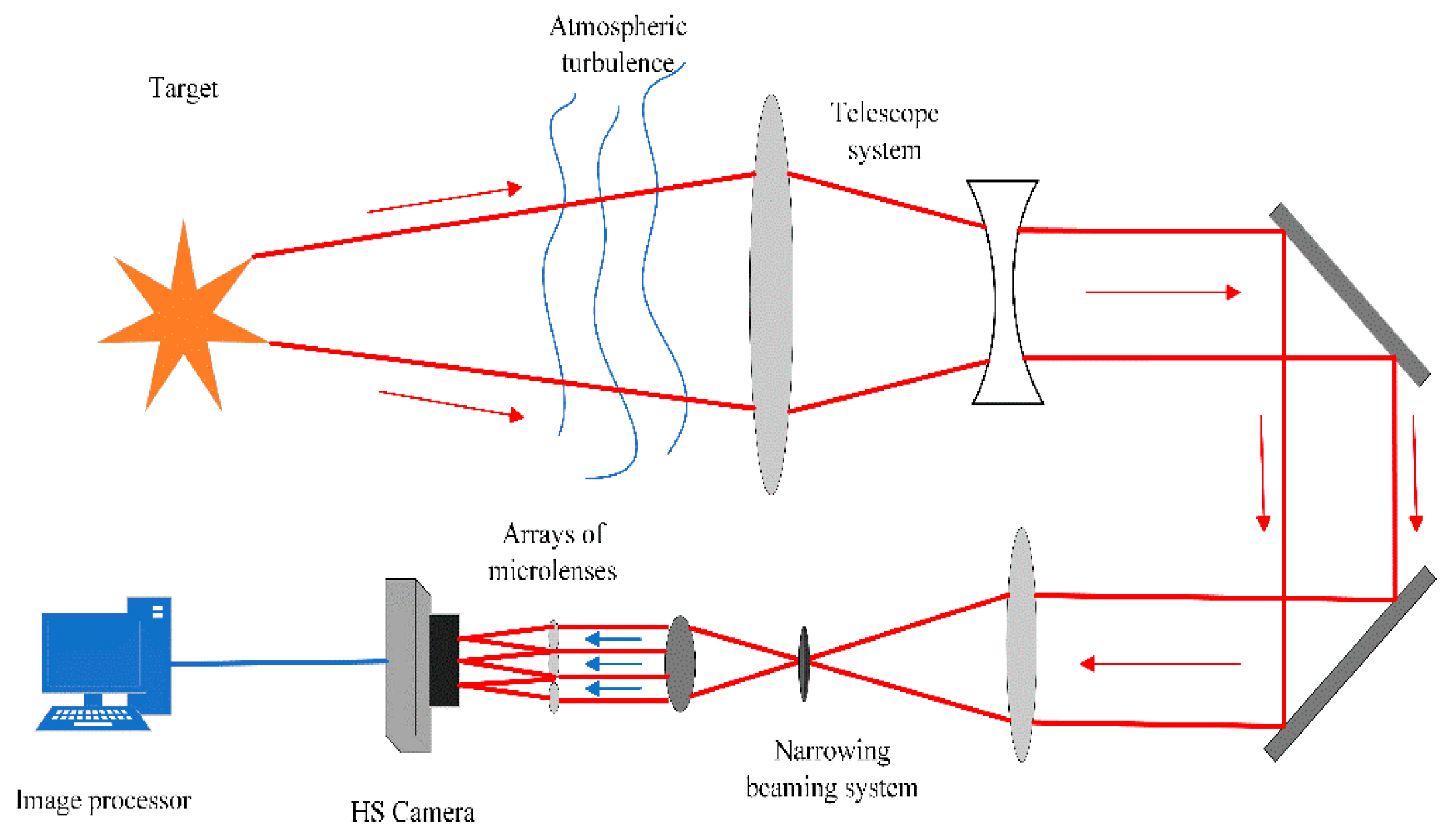
At present, there are two versions of the GPU-based SURF acceleration algorithm based on OpenCL and CUDA architecture. Because the CUDA architecture is managed within the development environment, the difficulty of programming is reduced. In this paper, we use the CUDA architecture to accelerate the SURF matching. The cross-correlation algorithm involved in this paper was implemented by using the Matlab 2022b, SURF acceleration software integrated development environment: Visual Studio 2015; open source library: CUDA 9.1, OpenCV 3.4.13; hardware platform: Intel (R) Core (TM) i5-8500 CPU @ 3.00 GHz; graphics: NVIDIA GeForce GTX 1650; operating system: Windows10.64 bit. The scene-based SHWS system is shown in Figure 10. It is mainly composed of a telescope system, beam shrinking system and Hartmann wavefront sensor. The total scaling magnification of the telescope system and the beam reduction system is 15 times, and the key parameters of the sensor are shown in Table 1.

3.1. SURF Application Simulation Based on CUDA Acceleration

According to the process of implementing the algorithm, the performance of feature detection is related to the resolution of the input image, and the computational complexity of the feature descriptor is related to the number of feature points detected. Therefore, in order to verify the accuracy of the algorithm in this paper, a comparative experiment between the traditional SURF algorithm and the optimized algorithm in this paper is designed. The reference image in Figure 1 is selected as the object scene, as shown in Figure 11 and Table 1 and Table 2. The running times of the feature point detection and feature point description processes for the four groups of images with different resolutions are recorded, respectively.
According to the judgment index in Mikolajczykz’s study [24], precision is used as the quantitative evaluation standard of the feature extraction method, as follows:
Accuracy = The   correct   feature   descriptor incorrect + correct
precision = correct incorrect + correct
It can be seen from Table 2 that the running time of the feature detection process increases with the increase in the image resolution, and the traditional serial algorithm is particularly time-consuming. The algorithm used in this paper is the same as the traditional detection feature points algorithm, and its detection accuracy can be as high as 99.77% according to Equation (15). For images with a resolution of 32 × 32, its complexity is low, the number of detected feature points is small, the algorithm running time is short and the detection accuracy can reach 100%. It can be seen that the algorithm in this paper greatly optimizes the feature detection speed while ensuring the detection accuracy.
As shown in Table 3, the running time for four sets of image feature description steps with different resolutions is recorded. It can be seen that the running time of the feature description process increases with the increase in the number of image detection feature points, especially when using the traditional SURF algorithm. accuracy of the generated feature descriptor is calculated according to Formula 16. Compared with the traditional SURF, the accuracy of the feature descriptor obtained by the algorithm in this paper is as high as 97.97%, and the optimization of SURF greatly reduces the time needed for the feature description.
Based on the above experimental process, the total time consumption and acceleration ratio of the optimization algorithm and the traditional SURF (As shown in Table 4) are calculated. With the increase in resolution, the traditional SURF takes a lot of time, while the optimization algorithm can achieve an average acceleration ratio of more than 10 times for images with different resolutions, and the acceleration effect is better. However, with the increase in image resolution and image complexity, the number of detected feature points increases, the degree of parallelism of the algorithm increases, and the parallel computing ability of the GPU is also enhanced. When the resolution and the number of feature points increase to a certain extent, GPU memory competition leads to a gradual decrease in the acceleration.

3.2. Simulation of the Shifts Based between Two Sub-Images

In order to verify the improvement in the shift result caused by the partial loss of the sub-image by using the above SURF matching method, two independent sub-images were used for evaluation. As shown in Figure 12, the reference image was set to be whole, and the sub-image was partially absent.
Since the wavefront separated by the microlens array can be considered to contain only tilt aberrations, in the simulation analysis of single sub-aperture shifts sensing, the shift of a single sub-image can be obtained by the diffraction spot and object image formed by the convolution tilt wavefront through the microlens. Therefore, the shift in the sub-image is simulated by changing the PV (peak-valley) value of the tilted wavefront corresponding to the sub-aperture.
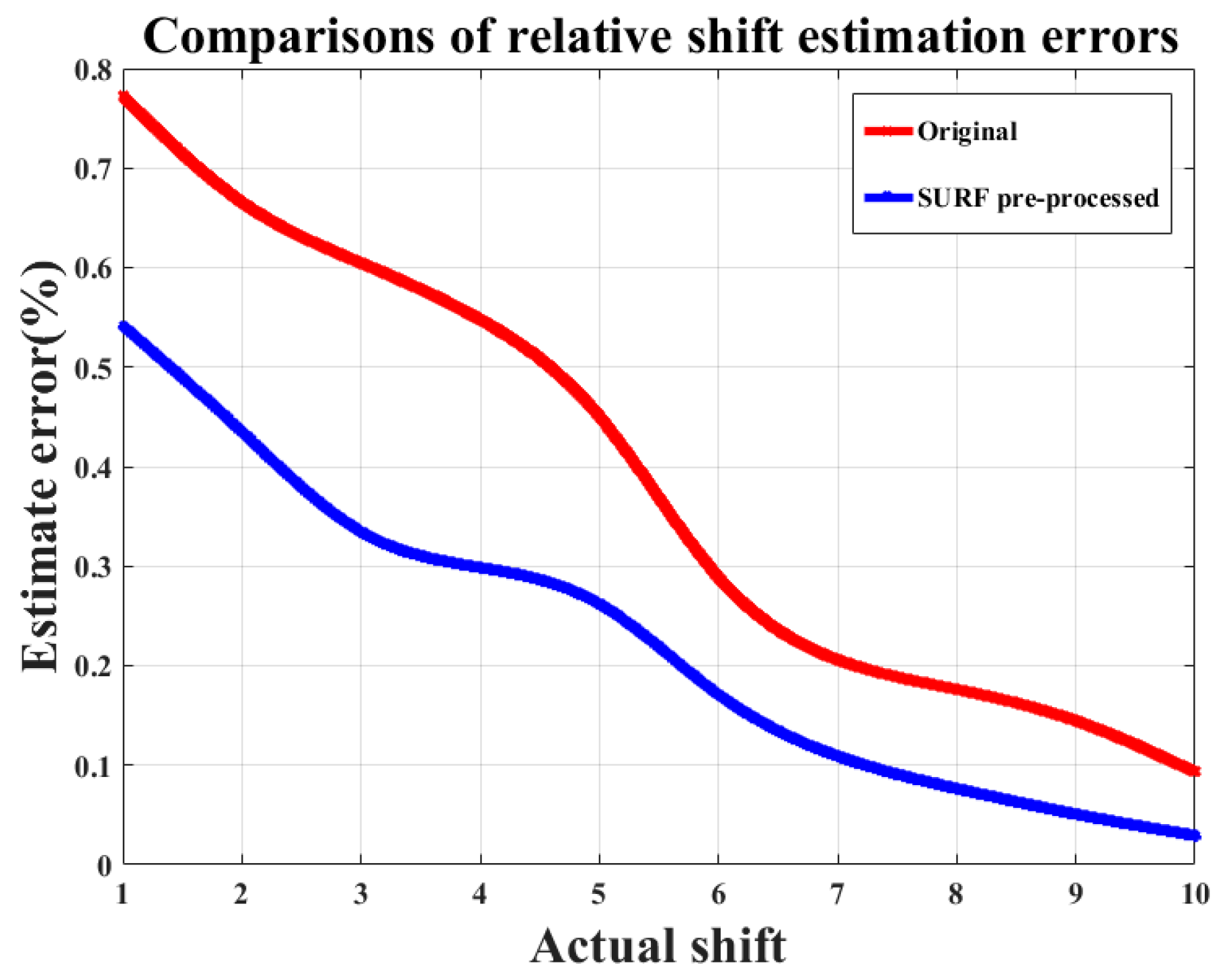
Ten sub-images with different unit pixel shifts based on the reference image were generated. The SURF pre-processed sub-image and the unprocessed sub-image have been used to calculate and compare the sub-aperture shifts. The results are shown in Figure 13.
The estimation error is defined as (calculated shift-actual shift) / actual shift. It can be seen that, compared with the unprocessed sub-image, the estimated error in the shift of the sub-image is reduced after the SURF pre-processing is applied to the sub-image. With the increase in the actual shift, the estimated error decreases, which is consistent with the conclusion that SURF will increase the correlation between the reference image and the sub-image.

3.3. Simulation of the Shifts Based on SURF Optimization

The Hartmann wavefront sensor needs to calculate the shift in about 100~200 sub-images for each wavefront sensing. A total of 169 sub-apertures are shown in Figure 14. If all sub-images are pre-processed before each shift calculation, even the basic image processing will take on the burden the realization of real-time wavefront sensing. In actual sensing, partial image absence often occurs at the edge of the sub-aperture. Therefore, we chose to process only 34 sub-apertures of the edge in this paper, which greatly reduced the calculation cost. As shown in Table 5, for a Hartmann wavefront sensor with 169 sub-apertures, each sub-aperture has 64 × 64 pixels. If SURF pre-processing is performed on all sub-images, the time required to calculate the shift of all sub-images at a time will be 1.7 times that without pre-processing. If only the edge sub-images are processed, the calculation cost can be reduced by 0.8 times.
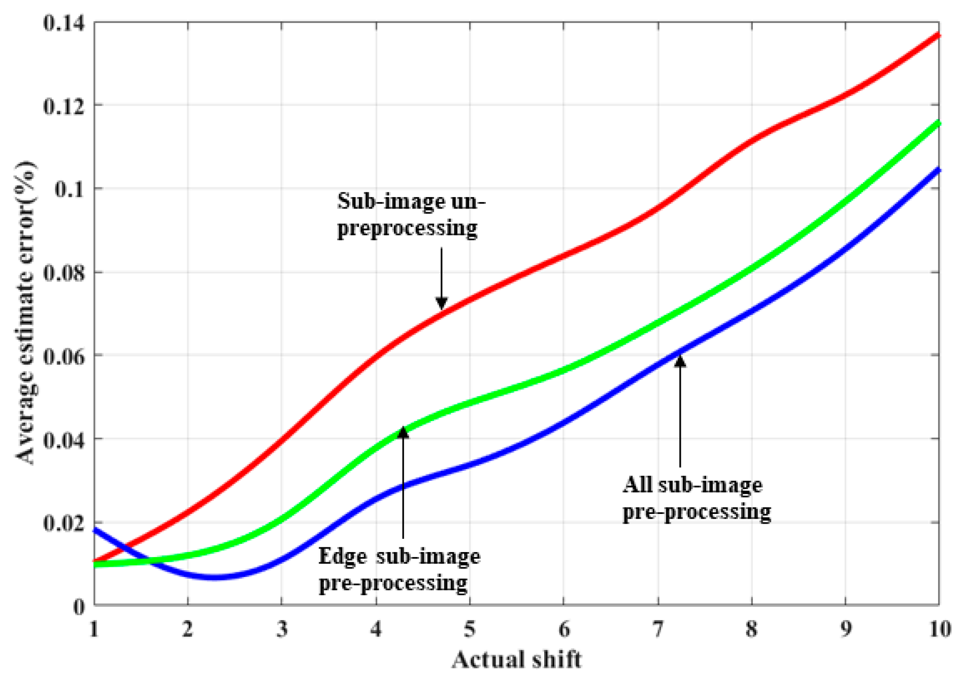
On this basis, in order to further verify the speed and accuracy of the optimized SURF in Section 3.1 in Hartmann sensing, the migration of 169 sub-images is simulated by changing the peak-valley value of the tilted wave surface corresponding to the sub-aperture. The shift is the same as the ten sets of simulation data in Section 3.2, and the 34 sub-images at the edge are partially absent. The results are shown in Figure 15.
It can be seen that only SURF preprocessing the edges of sub-images can still reduce the estimated error of sub-aperture shift. In the case of a large shift, the error results of the edge sub-image processing and the error results of all sub-image processing are nearly two times lower than the unprocessed error results, and the error results for edge sub-image processing are slightly higher than those for sub-image processing of the whole images, but more than half of the calculation cost is saved.
Therefore, for the wavefront sensing of partially absent sub-images, this paper proposes a wavefront sensing method that performs SURF-accelerated matching preprocessing on the edges of the sub-image and the reference image before the sub-image cross-correlation calculation.

4. Conclusions

In this paper, a cross-correlation algorithm based on SURF parallel acceleration for Shack–Hartmann wavefront sensing is proposed. To meet the speed required wavefront sensing, parallel optimization of SURF matching is carried out in CUDA using a GPU thread execution model and a programming model. Through the parallel acceleration optimization of the steps of calculating the Hessian response, non-maximum suppression, calculating the main direction of feature points and generating feature descriptors, the performance of SURF matching was improved. This method temporarily enhanced the shift result accuracy when the object plane of the sub-image is partially absent. A series of numerical simulations show that the shift error can be reduced by more than two times, and the parallel algorithm can achieve nearly ten times the acceleration ratio. Due to its excellent performance in eliminating partial image loss, it can be used as an important computational centroid algorithm to broaden the application range of scene-based AO systems.

Author Contributions

Conceptualization, L.W., X.M. and Y.T.; methodology, cand Z.Z.; software, L.W., X.M. and Z.Z.; validation, L.W., X.M., Z.Z. and F.C.; formal analysis, L.W., X.M. and Z.Z.; investigation, L.W., X.M., F.C. and J.W.; resources, Y.T., S.W. and P.Y.; data curation, L.W., X.M., F.C. and J.W.; writing—original draft preparation, L.W.; writing—review and editing, L.W., X.M. and Y.T.; visualization, L.W. supervision, L.W. and Y.T.; project administration, Y.T., S.W. and P.Y.; All authors have read and agreed to the published version of the manuscript.

Funding

This research received no external funding.

Institutional Review Board Statement

This study did not require ethical approval.

Informed Consent Statement

This study did not require ethical approval.

Data Availability Statement

Data are contained within the article.

Conflicts of Interest

The authors declare no conflicts of interest.

References

  1. Rao, C.H.; Zhang, X.J.; Jiang, W.H. Simulation of Hartmann-Shaker wavefront sensing for solar grain structure correlation. Acta Opt. Sin. 2002, 22, 285–289. [Google Scholar]
  2. Wizinowich, P.; Acton, D.S.; Shelton, C.; Stomski, P.; Gathright, J.; Ho, K.; Lupton, W.; Tsubota, K.; Lai, O.; Max, C.; et al. First light adaptive optics images from the Keck II telescope: A new era of high angular resolution imagery. Publ. Astron. Soc. Pac. 2000, 112, 315–319. [Google Scholar] [CrossRef]
  3. Booth, M.J. Adaptive optical microscopy: The ongoing quest for a perfect image. Light Sci. Appl. 2014, 3, e165. [Google Scholar] [CrossRef]
  4. Baum, M.; Hanebeck, U.D. Extended object tracking with random hypersurface models. IEEE Trans. Aerosp. Electron. Syst. 2014, 50, 149–159. [Google Scholar] [CrossRef]
  5. Keller, C.U.; Plymate, C.; Ammons, S.M. Low-cost solar adaptive optics in the infrared. In Innovative Telescopes and Instrumentation for Solar Astrophysics, Proceedings of the Astronomical Telescopes and Instrumentation, Waikoloa, HI, USA, 22–28 August 2002; International Society for Optics and Photonics: Bellingham, WA, USA, 2003; Volume 4853, pp. 351–359. [Google Scholar]
  6. Poyneer, L.A. Scene-based Shack-Hartmann wave-front sensing: Analysis and simulation. Appl. Opt. 2003, 42, 5807–5815. [Google Scholar] [CrossRef] [PubMed]
  7. Montmerle Bonnefois, A.; Fusco, T.; Meimon, S.; Mugnier, L.; Sauvage, J.F.; Engel, C.; Escolle, C.; Ferrari, M.; Hugot, E.; Liotard, A.; et al. Comparative theoretical and experimental study of a Shack-Hartmann and a Phase Diversity Sensor, for high-precision wavefront sensing dedicated to Space Active Optics. Proc. SPIE 2014, 10563, 105634B. [Google Scholar]
  8. Rimmele, T.R.; Radick, R.R. Solar Adaptive Optics at the National Solar Observatory. In Adaptive Optical System Technologies; Bonaccini, D., Tyson, R.K., Eds.; Proc. SPIE: Bellingham, WA, USA, 1998; Volume 3353, pp. 72–81. [Google Scholar]
  9. Poyneer, L.A.; Palmer, D.W.; LaFortune, K.N.; Bauman, B. Experimental results for correlation-based wavefront sensing. In Advanced Wavefront Control: Methods, Devices, and Applications III, Proceedings of the Optics and Photonics, San Diego, CA, USA, 31 July–4 August 2005; International Society for Optics and Photonics: Bellingham, WA, USA, 2005; Volume 5894, p. 58940N. [Google Scholar]
  10. Hu, X.Q.; Yu, X.; Zhao, D.Z. Effect of object image structure and noise on the sensing accuracy of correlated Hartmann-Shaker wavefront. Acta Opt. Sin. 2007, 27, 1414–1418. [Google Scholar]
  11. Sidick, E.; Green, J.J.; Morgan, R.M.; Ohara, C.M.; Redding, D.C. Adaptive cross-correlation algorithm for extended scene Shack-Hartmann wavefront sensing. Opt. Lett. 2008, 33, 213–215. [Google Scholar] [CrossRef] [PubMed]
  12. Sidick, E. Adaptive periodic-correlation algorithm for extended scene shack-hartmann wavefront sensing. In Proceedings of the Calculational Optical Sensing and Imaging, Toronto, ON, Canada, 10–14 July 2011; Optical Society of America: Washington, DC, USA, 2011; p. CPDP1. [Google Scholar]
  13. Wang, Y.W. Research on Related Hartmann Wavefront Detection Based on Extended Objects. Ph.D. Thesis, University of Chinese Academy of Sciences, Beijing, China, 2019. [Google Scholar]
  14. Yang, L.L. Research on Wave-Front Detection Technique of Variable Extensibility Object Based on Correlation Hartmann. Ph.D. Thesis, University of Chinese Academy of Sciences, Beijing, China, 2019. [Google Scholar]
  15. Wang, Y.; Chen, X.; Cao, Z.; Zhang, X.; Liu, C. Gradient cross-correlation algorithm for scene-based shack-hartmann wavefront sensing. Opt. Express 2018, 26, 17549. [Google Scholar] [CrossRef] [PubMed]
  16. Li, X.; Wu, Y.; Fang, Z.; Xu, Q.; Yang, H.-b.; Yang, H.-z. Post Processing for Adaptive Optics Imaging Based on Multi-channel Blind Recognition. Acta Photonica Sin. 2020, 49, 0201003. [Google Scholar]
  17. Bay, H.; Tuytelaars, T.; Van Gool, L. Surf: Speeded up robust features. In Computer Vision-ECCV 2006, Proceedings of the 9th European Conference on Computer Vision, Graz, Austria, 7–13 May 2006; Springer: Berlin/Heidelberg, Germany, 2006; pp. 404–417. [Google Scholar]
  18. Bay, H.; Ess, A.; Tuytelaars, T.; Van Gool, L. Speeded-up robust features (SURF). Comput. Vis. Image Underst. 2008, 110, 346–359. [Google Scholar] [CrossRef]
  19. Li, D. Feature Extraction and Object Recognition of Extended Objects. Ph.D. Thesis, Graduate School of Chinese Academy of Sciences, Institute of Optoelectronics Technology, Chengdu, China, 2013. [Google Scholar]
  20. Niu, T.; Liu, L.; Wu, Y. An image registration algorithm based on CUDA acceleration. Comput. Syst. Appl. 2023, 32, 146–155. [Google Scholar]
  21. Nakov, O.; Mihaylova, E.; Lazarova, M.; Mladenov, V. Parallel image stitching based on multithreaded processing on GPU. In Proceedings of the 2018 International Conference on Intelligent and Innovative Computing Application (ICONIC), Mon Tresor, Mauritius, 6–7 December 2018; IEEE: New York, NY, USA, 2018; pp. 1–5. [Google Scholar]
  22. Ding, P.; Wang, F.; Gu, D.Y.; Zhou, H.; Gao, Q.; Xiang, X. Research on optimization of SURF algorithm based on embedded CUDA platform. In Proceedings of the 2018 IEEE 8th Annual International Conference on CYBER Technology in Automation, Control, and Intelligent Systems (CYBER), Tianjin, China, 19–23 July 2018; IEEE: New York, NY, USA, 2018; pp. 1351–1355. [Google Scholar]
  23. Na, Y.; Liao, M.M.; Jung, C. Super-speed up robust features image geometrical registration algorithm. IET Image Process. 2016, 10, 848–864. [Google Scholar] [CrossRef]
  24. Mikolajczyk, K. A comparison of affine region detectors. Int. J. Comput. Vis. 2005, 65, 43–72. [Google Scholar] [CrossRef]
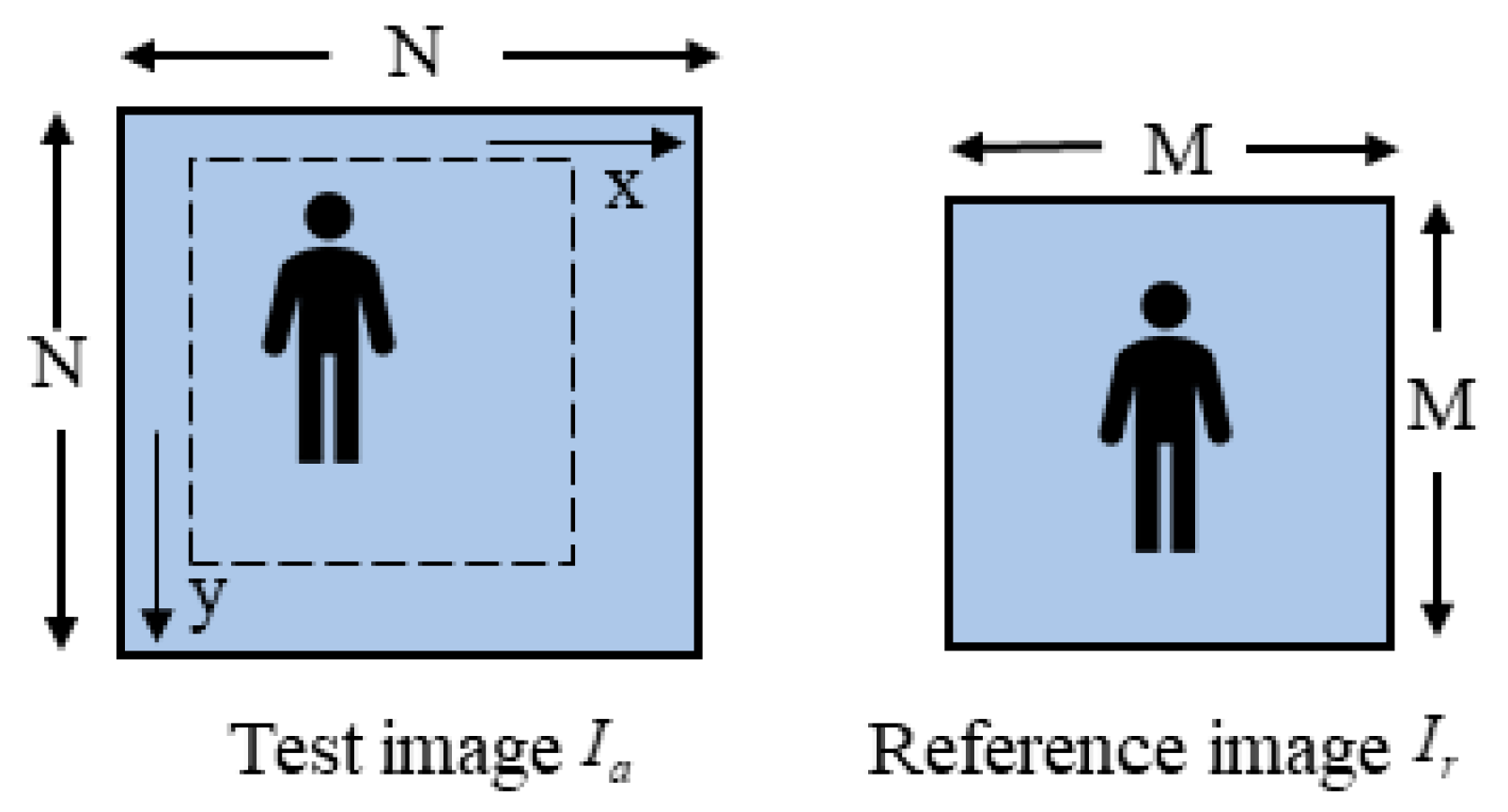
Figure 1. Matching process of the actual image and reference image.
Photonics 11 00844 g001
Figure 2. Influence of partial absence of sub-image on cross-correlation algorithm.
Photonics 11 00844 g002
Figure 3. SURF matching before cross-correlation algorithm.
Photonics 11 00844 g003
Figure 4. Integral image.
Photonics 11 00844 g004
Figure 5. Gaussian second derivative template.
Photonics 11 00844 g005
Figure 6. Approximation of Gaussian second derivative (box filter).
Photonics 11 00844 g006
Figure 7. Non-maximum suppression of a 3 × 3 × 3 neighborhood.
Photonics 11 00844 g007
Figure 8. The main direction determination diagram.
Photonics 11 00844 g008
Figure 9. Scheme of the SURF matching parallel acceleration optimization.
Photonics 11 00844 g009
Figure 10. Diagram of the optimal path in the experiment.
Photonics 11 00844 g010
Figure 11. Test images of different resolutions.
Photonics 11 00844 g011
Figure 12. Feature point registration process.
Photonics 11 00844 g012
Figure 13. Comparisons of relative shift estimation errors between pre-processing of SURF and unprocessed sub-images.
Photonics 11 00844 g013
Figure 14. Partial sub-apertures of the image.
Photonics 11 00844 g014
Figure 15. Average estimates of the error in pre-pressing and un-preprocessing sub-images.
Photonics 11 00844 g015
Table 1. Parameters of Shack–Hartmann wavefront sensor simulator.
ParametersValueParametersValue
Zernike order20Reference image size48 × 48 pixel
Incident wavelength1064 nmPixel size8 µm
Microlens focal length8 mmSub-aperture resolution64 × 64 pixel
Number of microlenses13 × 13Entrance pupil diameter4 mm
Table 2. SURF to detect feature points process comparison.
Traditional SURF Optimized SURF
Resolution RatioPoint NumberTime (ms)Point Number Time (ms)Precision
64 × 645842.3458 5.450.9977
48 × 483928.39393.770.9768
32 × 322715.11271.491.0000
24 × 24167.83160.970.8544
Table 3. Time comparison of feature description process.
Resolution RatioPoint NumberTraditional SURF (ms)Optimized SURF (ms)Precision
64 × 645849.354.150.8453
48 × 483914.681.660.7891
32 × 32276.371.230.9797
24 × 24160.890.0690.8905
Table 4. Results before and after SURF optimization.
Resolution RatioTraditional SURF (ms)Optimized SURF (ms)Speed-Up Ratio
64 × 64198.0521.159.42
48 × 48112.6716.756.72
32 × 3287.479.339.37
24 × 2456.766.988.13
Table 5. One-time wavefront sensing time of two different wavefront sensing methods.
Cross-Correlation AlgorithmAll Sub-Image PreprocessingEdge Sub-Image PreprocessingUn-Preprocessing
Calculation time/s0.1630.1100.097
Disclaimer/Publisher’s Note: The statements, opinions and data contained in all publications are solely those of the individual author(s) and contributor(s) and not of MDPI and/or the editor(s). MDPI and/or the editor(s) disclaim responsibility for any injury to people or property resulting from any ideas, methods, instructions or products referred to in the content.