Abstract
Coded aperture 3D imaging techniques have been rapidly evolving in recent years. The two main directions of evolution are in aperture engineering to generate the optimal optical field and in the development of a computational reconstruction method to reconstruct the object’s image from the intensity distribution with minimal noise. The goal is to find the ideal aperture–reconstruction method pair, and if not that, to optimize one to match the other for designing an imaging system with the required 3D imaging characteristics. The Lucy–Richardson–Rosen algorithm (LR2A), a recently developed computational reconstruction method, was found to perform better than its predecessors, such as matched filter, inverse filter, phase-only filter, Lucy–Richardson algorithm, and non-linear reconstruction (NLR), for certain apertures when the point spread function (PSF) is a real and symmetric function. For other cases of PSF, NLR performed better than the rest of the methods. In this tutorial, LR2A has been presented as a generalized approach for any optical field when the PSF is known along with MATLAB codes for reconstruction. The common problems and pitfalls in using LR2A have been discussed. Simulation and experimental studies for common optical fields such as spherical, Bessel, vortex beams, and exotic optical fields such as Airy, scattered, and self-rotating beams have been presented. From this study, it can be seen that it is possible to transfer the 3D imaging characteristics from non-imaging-type exotic fields to indirect imaging systems faithfully using LR2A. The application of LR2A to medical images such as colonoscopy images and cone beam computed tomography images with synthetic PSF has been demonstrated. We believe that the tutorial will provide a deeper understanding of computational reconstruction using LR2A.
1. Introduction
Imaging refers to the process of capturing and reproducing the characteristics of an object as close as possible to reality. There are two primary approaches to imaging: direct and indirect. Direct imaging is the oldest imaging concept, while indirect imaging is relatively much younger. A direct imaging system, as the name suggests, creates the image of an object directly on a sensor. Most of the commonly available imaging systems, such as laboratory microscopes, digital cameras, telescopes, and even the human eye, are based on the direct imaging concept. The indirect imaging concept requires at least two steps to complete the imaging process [1]. Holography is an example of the indirect imaging concept, and it consists of two steps, namely optical recording and numerical reconstruction. While the imaging process of holography is complicated and the setup is expensive when compared to that of direct imaging, the advantages in holography are remarkable. In holography, it is possible to record the entire 3D information of an object with a single camera shot in a 2D matrix. In direct imaging, a single camera shot can obtain only 2D information of an object. With holography, it is possible to record phase information, which enables seeing thickness and refractive index variations in transparent objects. The above significant advantages justify the complicated and expensive recording set up and two-step imaging process of holography [2].
In coherent holography, light from an object is interfered with a reference wave that has no information of the object but is derived from the same source to obtain the hologram. The above hologram recording process is suitable only if the illumination source is a coherent one [3]. Most of the commonly available imaging systems like the ones pointed out—laboratory microscopes, telescopes, and digital cameras—rely on incoherent illumination. There are many reasons for choosing incoherent illumination over coherent illumination, starting from the primary reason that it is not practical to shine a laser beam on any object, and natural light is incoherent. There are other advantages in incoherent imaging such as lesser imaging noise and higher imaging resolution compared to coherent imaging. However, recording a hologram with an incoherent source is a challenging task and impossible in the framework of coherent holography. A new concept of interference is needed in order to realize holography with an incoherent source [4,5].
One of the aims of holography is to compress 3D information into a 2D intensity distribution. In coherent holography, it is achieved by interfering the object wave that carries the phase fingerprint with a reference wave derived from the same source. The above method converts the phase fingerprint into an intensity distribution. The 3D object wave can be reconstructed by illuminating the recorded intensity distribution’s amplitude or phase transmission matrix with the reference wave, either physically as in analog holography or numerically as in digital holography. The above mode of recording a hologram is not possible with incoherent illumination due to the lack of coherence. To realize holography with incoherent illumination, a new concept called self-interference was proposed, which means that light from any object point is coherent with respect to itself and therefore can coherently interfere [3,5]. Therefore, instead of interfering the object wave with a reference wave, the object wave from every object point can be interfered coherently with the object wave from the same point for incoherent holography. The temporal coherence can be improved by trading off some light using a spectral filter. In this line of research, there have been many interesting architectures, such as rotational shearing interferometer [6,7,8], triangle interferometer [9,10], and conoscopic holography [11,12]. The modern-day incoherent holography approaches based on SLM [6,7,8,9,10,11,12] are Fresnel incoherent correlation holography (FINCH) [13,14] and Fourier incoherent single-channel holography [15,16], developed by Rosen and team. The field of incoherent holography rapidly evolved with advancements in optical configuration, recording, and reconstruction methods through the contributions of many researchers, such as Poon, Kim, Tahara, Matoba, Nomura, Nobukawa, Bouchal, Huang, Kner, and Potcoava [17,18]. Even with all the advancements, the latest version of FINCH required at least two camera shots and required multiple optical components [19,20].
In FINCH, light from an object point is split into two, differently modulated by two diffractive lenses, and interfered to record the hologram. The object’s image is reconstructed by Fresnel backpropagation [13]. A variation of FINCH called coded aperture correlation holography (COACH) was developed in 2016, where instead of one of the two diffractive lenses, a quasi-random scattering mask was used [21]. The reconstruction in COACH is also different from that of FINCH, as Fresnel backpropagation is not possible due to the lack of an image plane. Therefore, in COACH, the point spread hologram is recorded using a point object in the first step, which is then cross-correlated with the object hologram to reconstruct the image of the object. This type of reconstruction is common in coded aperture imaging (CAI) [22,23]. The origin of CAI can be traced back to the motivation of developing imaging technologies for non-visible regions of the electromagnetic spectrum, such as X-rays, Gamma rays, etc., where the manufacturing of lenses is a challenging task. In such cases, the light from an object was modulated by a random array of pinholes created on a plate made of a material that is not transparent to that radiation [22,23]. The point spread function (PSF) is recorded in the first step, the object intensity distribution is recorded next, and the image of the object is reconstructed by processing the two intensity patterns in the computer.
While CAI was used for recording 2D spatial and spectral information, it was not used for recording 3D spatial information as in holography [24]. With the development of COACH, a cross-over point between holography and CAI was identified, which led to the development of interferenceless COACH (I-COACH) [25]. In I-COACH, light from an object is modulated by a quasi-random phase mask and the intensity distribution is recorded. But instead of a single PSF, a PSF library is recorded, corresponding to different axial locations. This new approach connected incoherent holography with CAI. Since I-COACH with a quasi-random phase mask resulted in a low SNR, the next direction of research was set on the engineering of phase masks to maximize the SNR. Different phase masks were designed and tested for I-COACH for the generation of dot patterns [26], Bessel patterns [27], Airy patterns [28], and self-rotating patterns [29]. The above studies also revealed some unexpected capabilities of I-COACH, such as the capability to tune axial resolution independent of lateral resolution. Another direction of development in I-COACH was on improving the computational reconstruction method. The first version of I-COACH used a matched filter for processing PSF and object intensity distributions. Later, a phase-only filter was applied to improve the SNR [30]. In the subsequent studies of I-COACH, a novel computational reconstruction method called non-linear reconstruction (NLR) was developed whose performance was significantly better than both matched and phase-only filters [31]. An investigation was undertaken to understand if NLR is a universal reconstruction method for all optical fields with semisynthetic studies for a single plane, and the results were promising [32]. However, additional techniques, such as raising images to the power of p and median filters, were necessary to obtain a reasonable image reconstruction for deterministic optical fields [33].
Recently, a novel computational reconstruction method called the Lucy–Richardson–Rosen algorithm (LR2A) was developed by combining the well-known Lucy–Richardson algorithm (LRA) with NLR [34,35,36]. The performance of LR2A was found to be significantly better than LRA and NLR in many studies [37,38,39]. In this tutorial, we present the possibilities of using LR2A as a generalized reconstruction method for deterministic as well as random optical fields for incoherent 3D imaging applications. The physics of optical fields when switching from a coherent source to an incoherent source is different [40,41]. Many optical fields, such as Bessel, Airy, and vortex beam, have unique spatio-temporal characteristics that are useful for many applications. However, they cannot be used for imaging applications, as the above fields do not have a point focus. In this tutorial, we discuss the procedure for transferring the exotic 3D characteristics of the above special beams for imaging applications using LR2A. For the first time, the optimized computational MATLAB codes for implementing LR2A are also provided (see Supplementary Materials). The manuscript consists of six sections. The methodology is described in the second section. The third section contains the simulation studies. The experimental studies are presented in the fourth section. In the fifth section, an interesting method to tune axial resolution is discussed. The conclusion and future perspectives of the study are presented in the final section.
2. Materials and Methods
The aim of this tutorial is to show the step-by-step procedure on how to faithfully transfer the 3D axial characteristics present in exotic beams to imaging systems using the indirect imaging concept and LR2A. There have been many recent studies that have achieved this in the framework of I-COACH [42,43]. In the above studies, NLR has been used for reconstruction. It performs best with scattered distributions, and so in both studies, the deterministic fields’ axial characteristics have been transferred to the imaging system with additional sparsely random encoding. The optical configuration of the proposed system is shown in Figure 1. Light from an object is incident on a phase mask and recorded by an image sensor. The point spread function (PSF) is pre-recorded and used as the reconstructing function to obtain the object information. There are numerous methods available to process the object intensity distribution with the PSF; these include matched filter, phase-only filter, inverse filter, NLR, and LR2A. In this study, LR2A has been used, and it has a better performance than other methods when deterministic optical fields are considered.
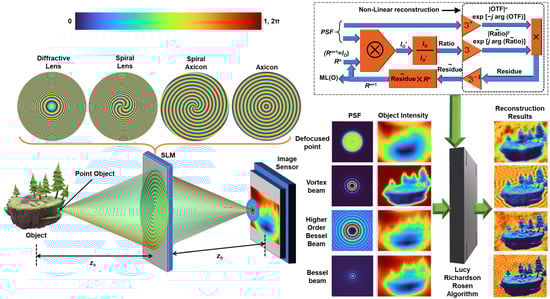
Figure 1.
Concept figure: recording images with different phase masks—diffractive lens, spiral lens, spiral axicon and axicon, and reconstruction using LR2A by processing object intensity and PSF. OTF—Optical transfer function; n—number of iterations; ⊗—2D convolutional operator; —complex conjugate following a Fourier transform;
—Inverse Fourier transform; Rn is the nth solution and n is an integer, when n = 1, Rn = I; ML—Maximum Likelihood; α and β are varied from −1 to 1.
The proposed analysis is limited to spatially incoherent illumination. The methods can be extended to coherent light when the object is a single point for depth measurements. A single point source with an amplitude of and located at is considered. The complex amplitude before the SLM is given as , where L is a linear phase function given as and Q is a quadratic phase function given as , where and C1 is a complex constant. In the SLM, the phase mask for the generation of an optical field is displayed. The phase function modulates the incoming light and the complex amplitude after the SLM is given as . At the image sensor, the recorded intensity distribution is given as
where is the location vector in the sensor plane, ‘⊗’ is a 2D convolutional operator, and propagates to the image sensor. For depth measurements, as mentioned above, both coherent as well as incoherent light sources can be used with a point object. In that case, it is sufficient to measure the correlation value at the origin obtained from , where Δz is the depth variation and ‘’ is a 2D correlation operator. The magnification of the system is given as MT = zh/zs. The lateral and axial resolution limits of the system for a typical lens are 1.22λzs/D and 8λ(zs/D)2, where D is the diameter of the SLM.
The IPSF can be expressed as
A 2D object with M point sources can be represented mathematically as M Kronecker Delta functions as
where are constants. In this study, only spatially incoherent illumination is considered, and so the intensity distribution of light diffracted from every point adds up in the sensor plane. Therefore, the object intensity distribution can be expressed as
In this study, the image reconstruction is carried out using LR2A, where the (n + 1)th reconstructed image is given as
where ‘’ refers to NLR, which is defined for two functions A and B as , where is the Fourier transform of X. The α and β are tuned between −1 and 1 to minimize noise. In the case of LRA, α and β are set to 1, which is a matched filter. The algorithm begins with an initial guess solution IO, which is a distorted version of O. In the first step, IO and IPSF are convolved to obtain the corresponding object intensity IO′ if IO is O. In the next step, the ratio between the original object intensity IO and obtained object intensity IO′ is calculated. This ‘Ratio’ is correlated with IPSF using NLR and the result is called the Residue. This ‘Residue’ is multiplied by the previous solution, which is IO after the first iteration and after the second iteration. The result gradually moves from IO towards O with every iteration. This process is iterated until an optimal reconstruction is obtained. There is a forward convolution and the ratio between this and is non-linearly correlated with . The better estimation from NLR enables a rapid convergence.
3. Simulation Results
In this tutorial, a wide range of phase masks are demonstrated as coded apertures, with some of them commonly used and some exotic. In the previous studies with LR2A, it was shown that the performance of LR2A is best when the IPSF is a symmetric distribution along the x and y directions [39,44]. The shift variance in LR2A was demonstrated [44]. Some solutions in the form of post-processing to address the problems associated with the asymmetry of the IPSF have been discussed in [39]. However, all the above effects were due to the fact that LR2A was not generalized. In this study, LR2A has been generalized to all shapes of IPSFs and both real and complex cases. The simulation space has been constructed in MATLAB with the following specifications: Matrix size = 500 × 500 pixels, pixel size Δ = 10 μm, wavelength λ = 650 nm, object distance zs = 0.4 m, recording distance zh = 0.4 m, and focal length of diffractive lens f = 0.2 m. For the diffractive lens, to prevent the direct imaging mode, the zh value was modified to 0.2 m. The phase masks of a diffractive lens, spiral lens, axicon, and spiral axicon are given as , , , , respectively, where L is the topological charge and Λ is the period of the axicon. The optical configuration in this study is simple, consisting of three steps, namely free space propagation, interaction, and again a free space propagation. The equivalent mathematical operations for the above three steps, propagation, interaction, and propagation, are convolution, product, and convolution, respectively. The first mathematical operation is quite direct, as a single point is considered; this constitutes a Kronecker Delta function. Any function convolved with a Delta function creates a replica of the function. Therefore, the complex amplitude obtained after the first operation is equivalent to . In the next step, the above complex amplitude is multiplied by by an element-wise multiplication operation. In the final step, the resulting complex amplitude is propagated to the sensor plane by a convolution operation expressed as three Fourier transforms . The intensity distribution IPSF can be obtained by squaring the absolute value of the complex amplitude matrix obtained at the sensor plane. The steps in the MATLAB software (Version 9.12.0.1884302 (R2022a)) can be found in the supplementary files of [45].
The simulation was carried out by shifting zs from 0.2 to 0.6 m in steps of 4 mm, and the IPSF(zs) was accumulated into a cube matrix (x, y, z, I). The images of the phase masks for diffractive lens, spiral lens (L = 1, 3, and 5), diffractive axicon, and spiral axicon (L = 1, 3, and 5) are shown in row 1 of Figure 2. The 3D axial intensity distributions for different diffractive elements, such as diffractive lens, spiral lens (L = 1, 3 and 5), diffractive axicon, and spiral axicon (L = 1, 3, and 5), are shown in row 2 of Figure 2. The diffractive lens does not have a focal point, as the imaging condition was not satisfied within this range of zs when zh is 0.2 m. For the spiral lens, a focused ring is obtained at the recording plane corresponding to zs = 0.4 m and the ring blurs and expands, similar to the case of a diffractive lens. For a diffractive axicon, a Bessel distribution is obtained in the recording plane and it is invariant with changes in zs [46,47]. A similar behavior is seen in Higher-Order Bessel Beams (HOBBs) [48]. As seen in the axial intensity distributions, none of the beams can be directly used for imaging applications. It may be argued that Bessel beams can be used, but as is known, the non-changing intensity distribution comes at a price, which is the loss of higher spatial frequencies [33]. Consequently, imaging using Bessel beams results in low-resolution images.
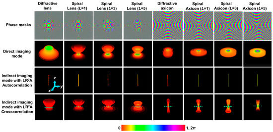
Figure 2.
Row 1: Phase masks of a diffractive lens, spiral lens (L = 1, 3, and 5), diffractive axicon, and spiral axicon (L = 1, 3, and 5). Row 2: Cube data of axial intensity distributions obtained at the recording plane for a diffractive lens, spiral lens (L = 1, 3, and 5), diffractive axicon, and spiral axicon (L = 1, 3, and 5). Row 3: Cube data of the intensity of the autocorrelation function for the different cases of phase masks. Row 4: Cube data of the cross-correlation function for the different cases of phase masks, when zs is varied from 0.2 to 0.6 m.
The holographic point spread function is not IPSF but , where ‘’ is the LR2A operator with n iterations, which is equivalent to the autocorrelation function. It must be noted that what is performed in LR2A is not a regular correlation as in a matched filter. The autocorrelation function was calculated for the above zs variation for the different cases of phase masks and accumulated in a cube matrix, as shown in the third row of Figure 2. As seen, the autocorrelation function is a cylinder with uniform radius for all values of zs. This is the holographic 3D PSF from whose profile it seems that it is possible to reconstruct the object information with a high resolution for all the object planes. To understand the axial imaging characteristics in the holographic domain, the IPSF(zs) was cross-correlated with IPSF of a reference plane, which in this case has been set at zs = 0.4 m. Once again, this cross-correlation is the nearest equivalent term in LR2A, which is calculated as . The cube data obtained for different phase masks are shown in the fourth row from the top in Figure 3. As seen in the figure, the axial characteristics have been faithfully transferred to the imaging system except that now it is possible to perform imaging at any one or multiple planes of interest simultaneously. With a diffractive lens, a focal point is seen at a particular plane and blurred in other planes with respect to zs. The same behavior can be observed about the spiral lenses which contains the diffractive lens function. The case of the axicon shows a long focal depth, and a similar behavior is seen for the cases of the spiral axicon. With the indirect imaging concept and LR2A, it is possible to faithfully transfer the exotic axial characteristics of special beams to an imaging system. It must be noted that the cross-correlation was carried out with fixed values of α, β, and n for every case. In some of the planes, there is some scattering seen, indicating either a non-optimal reconstruction condition or slightly lower performance of LR2A.
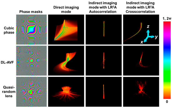
Figure 3.
Column 1: Phase images of cubic phase mask, DL-AVF, and quasi-random lens. Column 2: Cube data of axial intensity distributions obtained at the recording plane for cubic phase mask, DL-AVF, and quasi-random lens. Column 3: Cube data of the intensity of the autocorrelation function for the different cases of phase masks. Column 4: Cube data of the cross-correlation function for the different cases of phase masks, when zs is varied from 0.1 to 0.7 m.
All the above cases demonstrated consist of IPSFs that are radially symmetric. When considering asymmetric cases such as Airy beams, self-rotating beams, and speckle patterns, NLR performed better than LR2A, as it was not optimized for asymmetric cases. In this study, LR2A has been generalized for asymmetric shapes. Three phase masks—a cubic phase mask with a phase function , where a = b~1000 [28,40], a diffractive lens with azimuthally varying focal length (DL-AVF) [29,49], and a quasi-random lens with a scattering ratio of 0.04, obtained using the Gerchberg–Saxton algorithm [3] are investigated. The images of the phase masks for the above three cases are shown in column 1 in Figure 3. In this case, to show the curved path of the Airy pattern, the axial range was extended for zs from 0.4 m to 0.6 m. The 3D intensity distribution in the direct imaging mode for the three cases is shown in column 2 of Figure 3. The 3D autocorrelation distribution is shown in column 3 of Figure 3 for the three cases. The 3D cross-correlation distribution obtained by LR2A for the three cases is shown in column 4 of Figure 3. As seen from columns 2 and 4, the axial characteristics of the exotic beams have been faithfully transferred to the imaging system. The quasi-random lens or any scattering mask behaves exactly like a diffractive lens in the holographic domain. Comparing the results in Figure 3 and the previous results [39,44], a significant improvement is seen.
The simulation study of a two-plane object consisting of two test objects with letters “CIPHR” and “TARTU” with zs = 0.4 m and 0.5 m, respectively, is presented next. The images of the IPSFs for zs = 0.4 m and 0.5 m, the object intensity pattern IO obtained by convolution of object “CIPHR” with IPSF (zs = 0.4 m) and convolution of “TARTU” with IPSF (zs = 0.5 m) followed by a summation and the reconstructions IR corresponding to the two planes using LR2A for a diffractive lens, spiral lens (L = 5), spiral axicon (L = 3), cubic phase mask, DL-AVF, and quasi-random lens are shown in Figure 4. As seen from the results in Figure 4, the cases of the diffractive lens and quasi-random lens appear similar with respect to the axial behavior, i.e., when a particular plane information is reconstructed, only that plane information is focused and enhanced, while the other plane information is blurred and weak. However, for the elements such as the spiral lens and spiral axicon, the other plane information consists of “hot spots”, which are prominent and sometimes even stronger than the information in the reconstructed plane. This is due to the fact that there is similarity between the two IPSFs. This is one of the pitfalls of using such deterministic optical fields. The problem with such hotspots is that it is not possible to discriminate if the hotspot corresponds to any useful information related to the object or blurring due to a different plane if the object is not known prior.
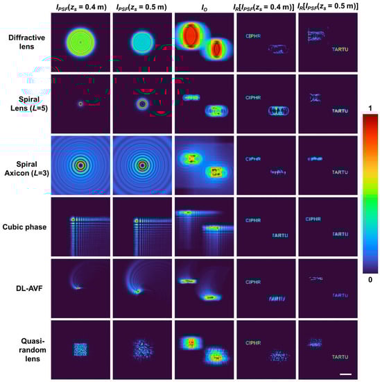
Figure 4.
Column 1: Images of IPSF (zs = 0.4 m), column 2: images of IPSF (zs = 0.5 m), column 3: object intensity distributions IO for the two-plane object consisting of “CIPHR” and “TARTU”, column 4: reconstruction results IR using column 1, column 5: reconstruction results IR using column 2, for diffractive lens (row 1), spiral lens (L = 5) (row 2), spiral axicon (L = 3) (row 3), cubic phase mask, DL-AVF (row 5), and quasi-random lens (row 6). Scale bar—1 mm.
Another pitfall in 3D imaging in the indirect imaging mode is the depth–wavelength reciprocity [33,50]. The changes in intensity distribution may appear identical to a change in depth or change in wavelength or both. This is true of both deterministic as well as random optical fields, except for beams carrying OAM, as a change in wavelength causes fractional topological charge, which is unique. Another point to consider when using IPSF from a special function is the sampling. Except for the cases of the quasi-random lens and diffractive lens, the other cases have distorted the object information in some ways. In the case of the Airy beam, the IPSF consists of periodic dot patterns along the x and y directions, which, when it samples the object information, the curves are sampled into square shapes. A ring-shaped IPSF has shaped the object information in this fashion, which again raises concerns about the reliability of the measurement, when the object information is not already known. In all the simulation studies, the optimal reconstructions were obtained for the following values: , , and .
4. Experiments
The schematic and photograph of the experimental setup are shown in Figure 5 and Figure 6, respectively. The setup was built using the following optical components: high-power LED (Thorlabs, 940 mW, λ = 660 nm and Δλ = 20 nm, Newton, MA, USA), iris, diffuser, polarizer, refractive lenses, object/pinhole, beam splitter, spatial light modulator (SLM) (Thorlabs Exulus HD2, 1920 × 1200 pixels, pixel size = 8 μm, Newton, MA, USA), and an image sensor (Zelux CS165MU/M 1.6 MP monochrome CMOS camera, 1440 × 1080 pixels with pixel size ~3.5 µm, Newton, MA, USA). The light from the LED was passed through the iris (I1), which controls the light illumination and then passed through a diffuser (Thorlabs Ø1” Ground Glass Diffuser-220 GRIT, Newton, MA, USA), which is used to remove the LED’s grating lines. The light from the diffuser was collected using a refractive lens (Lens1) (f = 5 cm), and it is passed through a polarizer, which is oriented along the active axis of the SLM. Two objects, digit ‘3’ and ‘1’, from Group-5 from R1DS1N—Negative 1951 USAF Test Target, Ø1”, were used. A pinhole of 50 μm was used to record the IPSF. The object is critically illuminated using a refractive lens (Lens2) (f = 5 cm). The light from the object is collimated by another refractive lens (Lens3) (f =5 cm) and passed through the beam splitter and incident on the SLM. On the SLM, phase masks of deterministic and random optical fields were displayed one after another, and the IPSF and IO were recorded by the image sensor.
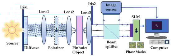
Figure 5.
Schematic of the experimental setup.
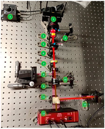
Figure 6.
Photograph of experimental setup: (1) LED, (2) LED power controller, (3) iris(I1), (4) diffuser, (5) refractive lens (L1), (6) polarizer, (7) refractive lens (L2), (8) object/pinhole, (9) refractive lens (L3), (10) iris (I2), (11) beam splitter, (12) SLM, (13) image sensor.
The experimental results for 2D imaging of USAF object ‘3’ using different methods such as matched filter, phase-only filter, NLR, and LR2A are presented in Figure 7. In Figure 7, the phase masks of the deterministic and random optical fields are shown in column 1 and their corresponding IPSFs and IOs (zs = 5 cm) are shown in columns 2 and 3, respectively. The reconstruction results of matched filter, phase-only filter, NLR, and LR2A are shown in columns 4 to 7 respectively. From Figure 7, the better performance of LR2A is evident. The structural similarity index measure (SSIM) and root mean square error (RMSE) are calculated for different optical fields and different reconstruction methods and the values are compared in a bar graph, as shown in Figure 8. As seen from Figure 8, we can conclude that the performance of LR2A is better than other reconstruction methods.
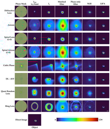
Figure 7.
Experimental results of 2D imaging. Column 1: Images of phase masks, column 2: images of IPSF (zs = 5 cm), column 3: images of object intensity distributions IO of the object at depth IO (zs = 5 cm). Reconstruction results by matched filter, phase-only filter, NLR, and LR2A in column 4, column 5, column 6, and column 7, respectively. Scale bar—50 μm.
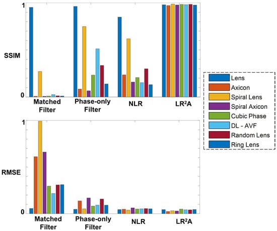
Figure 8.
Bar graph of SSIM and RMSE for different reconstruction methods such as matched filter, phase-only filter, NLR, and LR2A.
The IO values for two objects are recorded at two different depths (zs = 5 cm and zs = 5.6 cm) and summed to demonstrate 3D imaging. The 3D experimental results are presented in Figure 9. The IPSFs for zs = 5 cm and zs = 5.6 cm are shown in columns 1 and 2, respectively, in Figure 9. IO is shown in column 3 and IR by LR2A for zs = 5 cm and zs = 5.6 cm are shown in column 4 and column 5, respectively. Once again, it can be seen that the 3D characteristics of the beams have been faithfully transferred to the indirect imaging system. In all the experimental studies, the optimal reconstructions were obtained for the following values: , , and .
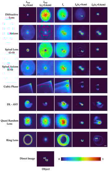
Figure 9.
Experimental results of 3D imaging. Column 1: images of IPSF (zs = 5 cm), column 2: images of IPSF (zs = 5.6 cm), column 3: images of summed object intensity distributions IO of the two objects at different depths IO (zs = 5 cm) and IO (zs = 5.6 cm), column 4: Reconstruction results IR (zs = 5 cm) using corresponding IPSF (zs = 5 cm) in column 1, column 5: Reconstruction results IR (zs = 5.6 cm) using corresponding IPSF (zs = 5.6 cm) in column 2. Scale bar—50 μm.
To demonstrate the application of LR2A to real applications in day-to-day life, medical images were obtained from surgeons. A male 65-year-old patient with a known case of prostrate cancer had radiotherapy about a year ago. He developed bleeding and mucous discharge from the anus. The colonoscopy finding shows mucosal pallor, telangiectasias, edema, spontaneous hemorrhage, and friable mucosa. It can be noted that the mucosa was congested with ulceration stricture. The images were captured using colonoscope Olympus system and CaptureITPro medical imaging software. The direct images obtained using the colonoscope are shown in Figure 10. The IPSF can be synthesized in a computer or an isolated dot can be taken from Figure 10, padded with zeros and used as the reconstructing function. The red region indicates telangiectasias and the black region shows necrosis, which is the death of body tissue. The yellow region shows mucosal sloughing, and the magnified region shows the necrotic area with dead mucosa. In this study, the IPSF was synthetic [38,39]. The different color channels were extracted from the image and processed separately using synthetic IPSF and different types of filters, such as matched filter, phase-only filter, NLR, and LR2A, and then combined as discussed in [38]. The NLR was carried out for α = 0 and β = 0.8 and LR2A was carried out for α = 0.2 and β = 1 with n = 20 iterations. The reconstructed images are shown in Figure 9, which shows that LR2A has a better performance compared to other methods.
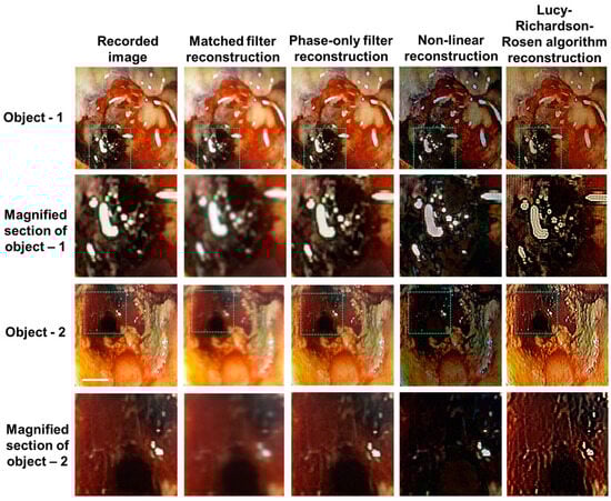
Figure 10.
Experimental colonoscopy results. Red region—telangiectasias; black region—necrosis, which is the death of body tissue; yellow region—mucosal sloughing; magnified region—necrotic area (dead mucosa). Reconstruction by matched filter, phase-only filter, NLR, and LR2A. The scale bar is 6 cm. The dotted areas are magnified in the subsequent row.
A diagnostic imaging equipment, Cone beam computed tomography (CBCT), was used for imaging a patient with focal spot 0.5 mm, field of view 8 × 8 cm, voxel size 0.2 mm/0.3 mm, and exposure time 15.5 s. The images obtained for a patient with multiple implants placed in the jaw with metallic artifacts compromised the clarity and blurred the finer details, as shown in row 1 of Figure 11. Once again, synthetic IPSF and LR2A were used to improve the resolution and contrast of the images. The images were reconstructed using different types of filters, such as matched filter, phase-only filter, NLR, and LR2A. The reconstructed images have a better resolution and contrast compared to the direct images. The NLR was carried out for α = 0 and β = 0.7 and LR2A was carried out for α = 0.3 and β = 1 with n = 20 iterations. The reconstructed images are shown in Figure 11, which shows that LR2A has a better performance compared to other methods.
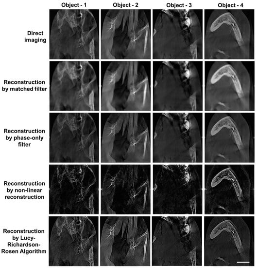
Figure 11.
Experimental cone beam computed tomography results of four objects. The saturated region indicates metal artifacts. The size of each square is 8 cm × 8 cm. Reconstruction by matched filter, phase-only filter, NLR, and LR2A. Scale bar is 2 cm.
5. Discussion
In this study, LR2A and the indirect imaging concept have been used as a tool to transfer the 3D imaging characteristics faithfully from the beam to the imaging system [42,43,51]. In our recent study [51], the possibility of tuning axial resolution of an imaging system after completing the recording process has been demonstrated by post hybridization methods. The same can be achieved with the common and exotic beams. A hybrid PSF IHPSF can be formed by summing the pure IPSFs with appropriate weights w in the following form: . The object intensity distribution can be hybridized by the same weights as used for creating the hybrid PSFs as . The object information can be reconstructed with the effective imaging characteristics using LR2A. Two cases are simulated here. In the first case, hybridization has been achieved between the Airy pattern and self-rotating beam, and in the second case, hybridization has been achieved between the Airy pattern and quasi-random lens. The 4D intensity distributions generated for the hybrid PSFs are shown in Figure 12a,c for cases 1 and 2, respectively. The reconstructed 4D patterns using LR2A for cases 1 and 2 are shown in Figure 12b,d, respectively. As expected, the focal depth decreased in the second case Figure 12d more than the first case Figure 12b, as the second ingredient in the second case has a high axial resolution. This study is not limited to only two ingredients, but any type of ensemble with m number of beams can be constructed easily post-recording.
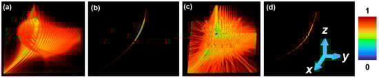
Figure 12.
Simulation results of post-hybridization: 4D distribution of hybrid beam obtained by combining (a) Airy beam and self-rotating beam and (b) its reconstruction using LR2A; 4D distribution of hybrid beam obtained by combining (c) Airy beam and scattered beam and (d) its reconstruction using LR2A.
6. Conclusions
In this tutorial, LR2A has been presented as a generalized computational reconstruction method for different types of deterministic fields and scattered patterns. The algorithm was also tested for a wide range of beams and variations, and it was always possible to obtain a high-quality reconstruction result by tuning the parameters α, β, and n. In all the cases, the axial characteristics have been faithfully transferred from the non-imaging beam to the imaging system using LR2A. Further, medical images recorded directly using a colonoscope and CBCT have been processed using synthetic IPSF and LR2A and an enhancement in resolution and contrast was observed. The method can be extended for aberration correction as well by choosing an aberrated dot from the recorded images. The above high-quality reconstructions in both laboratories set up with wide range of deterministic optical fields and scattered field and medical images demonstrate the wide applicability of LR2A, making it a universal computational reconstruction method.
Supplementary Materials
The following supporting information can be downloaded at: https://www.mdpi.com/article/10.3390/photonics10090987/s1, The MATLAB code for Lucy–Richardson–Rosen algorithm.
Author Contributions
Conceptualization, V.A.; methodology, V.A., A.N.K.R., R.A.G., M.S.A.S., S.D.M.T., A.P.I.X., F.G.A., S.G. and A.S.J.F.R.; software, V.A., M.S.A.S. and S.D.M.T.; validation, V.A., A.N.K.R., R.A.G., M.S.A.S., S.D.M.T., A.P.I.X., F.G.A., S.G. and A.S.J.F.R.; formal analysis, V.A., M.S.A.S. and S.D.M.T.; investigation, all the authors; resources, V.A., M.S.A.S. and S.D.M.T.; writing—original draft preparation, A.P.I.X., F.G.A. and V.A.; writing—review and editing, all the authors; supervision, V.A.; project administration, A.S.J.F.R.; funding acquisition, V.A., M.S.A.S. and S.D.M.T. All authors have read and agreed to the published version of the manuscript.
Funding
This research was funded by European Union’s Horizon 2020 research and innovation programme grant agreement No. 857627 (CIPHR). This work was partly supported by the European Regional Development Fund under Grant 1.1.1.5/19/A/003.
Informed Consent Statement
Informed consent was obtained for the medical images involved in the study. The informed consent has been obtained from the patients of Dr. Scott’s Laser Piles Fistula Center, Nagercoil, Tamil Nadu 629201, India, and Darshan Dental and Orthodontic Clinic, Kanyakumari, Tamil Nadu 629401, India, to publish this paper.
Data Availability Statement
The data can be obtained from the authors upon reasonable request.
Acknowledgments
The authors thank Dr. Scott’s Laser Piles Fistula Center, Dr. Jeyasekharan Hospital, Rajas Dental College and Hospital and Darshan Dental and Orthodontic Clinic, Kanyakumari, India.
Conflicts of Interest
The authors declare no conflict of interest.
References
- Goodman, J.W. Introduction to Fourier Optics, 3rd ed.; Roberts and Company: Englewood, CO, USA, 2005. [Google Scholar]
- Javidi, B.; Carnicer, A.; Anand, A.; Barbastathis, G.; Chen, W.; Ferraro, P.; Goodman, J.W.; Horisaki, R.; Khare, K.; Kujawinska, M.; et al. Roadmap on digital holography. Opt. Express 2021, 29, 35078–35118. [Google Scholar] [CrossRef] [PubMed]
- Rosen, J.; Vijayakumar, A.; Kumar, M.; Rai, M.R.; Kelner, R.; Kashter, Y.; Bulbul, A.; Mukherjee, S. Recent advances in selfinterference incoherent digital holography. Adv. Opt. Photonics 2019, 11, 1–66. [Google Scholar] [CrossRef]
- Liu, J.P.; Tahara, T.; Hayasaki, Y.; Poon, T.C. Incoherent digital holography: A review. Appl. Sci. 2018, 8, 143. [Google Scholar] [CrossRef]
- Rosen, J.; Vijayakumar, A.; Hai, N. Digital holography based on aperture engineering. In SPIE Spotlight E Book Series; Bellingham: Washington, DC, USA, 2023. [Google Scholar]
- Murty, M.V.R.K.; Hagerott, E.C. Rotational shearing interferometry. Appl. Opt. 1966, 5, 615–619. [Google Scholar] [CrossRef]
- Armitage, J.D.; Lohmann, A. Rotary shearing interferometry. Opt. Acta 1965, 12, 185–192. [Google Scholar]
- Roddier, C.; Roddier, F.; Demarcq, J. Compact rotational shearing interferometer for astronomical applications. Opt. Eng. 1989, 28, 280166. [Google Scholar] [CrossRef]
- Cochran, G. New method of making Fresnel transforms with incoherent light. J. Opt. Soc. Am. 1966, 56, 1513–1517. [Google Scholar] [CrossRef]
- Marathav, A.S. Noncoherent-object hologram: Its reconstruction and optical processing. J. Opt. Soc. Am. 1987, 4, 1861–1868. [Google Scholar] [CrossRef]
- Sirat, G.Y. Conoscopic holography. I. Basic principles and physical basis. J. Opt. Soc. Am. 1992, 9, 70–83. [Google Scholar] [CrossRef]
- Mugnier, L.M.; Sirat, G.Y. On-axis conoscopic holography without a conjugate image. Opt. Lett. 1992, 17, 294–296. [Google Scholar] [CrossRef]
- Rosen, J.; Brooker, G. Digital spatially incoherent Fresnel holography. Opt. Lett. 2007, 32, 912–914. [Google Scholar] [CrossRef] [PubMed]
- Rosen, J.; Brooker, G. Non-scanning motionless fluorescence three-dimensional holographic microscopy. Nat. Photon. 2008, 2, 190–195. [Google Scholar] [CrossRef]
- Kelner, R.; Rosen, J. Spatially incoherent single channel digital Fourier holography. Opt. Lett. 2012, 37, 3723–3725. [Google Scholar] [CrossRef] [PubMed]
- Kelner, R.; Rosen, J.; Brooker, G. Enhanced resolution in Fourier incoherent single channel holography (FISCH) with reduced optical path difference. Opt. Express 2013, 21, 20131–20144. [Google Scholar] [CrossRef] [PubMed]
- Rosen, J.; Alford, S.; Vijayakumar, A.; Art, J.; Bouchal, P.; Bouchal, Z.; Erdenebat, M.U.; Huang, L.; Ishii, A.; Juodkazis, S.; et al. Roadmap on recent progress in FINCH technology. J. Imaging 2021, 7, 197. [Google Scholar] [CrossRef]
- Tahara, T.; Zhang, Y.; Rosen, J.; Anand, V.; Cao, L.; Wu, J.; Koujin, T.; Matsuda, A.; Ishii, A.; Kozawa, Y.; et al. Roadmap of incoherent digital holography. Appl. Phys. 2022, 128, 193. [Google Scholar] [CrossRef]
- Tahara, T.; Kozawa, Y.; Ishii, A.; Wakunami, K.; Ichihashi, I.; Oi, R. Two-step phase-shifting interferometry for self-interference digital holography. Opt. Lett. 2021, 46, 669–672. [Google Scholar] [CrossRef]
- Siegel, N.; Lupashin, V.; Storrie, B.; Brooker, G. High-magnification super-resolution FINCH microscopy using birefringent crystal lens interferometers. Nat. Photon. 2016, 10, 802–808. [Google Scholar] [CrossRef]
- Vijayakumar, A.; Kashter, Y.; Kelner, R.; Rosen, J. Coded aperture correlation holography—A new type of incoherent digital holograms. Opt. Express 2016, 24, 12430–12441. [Google Scholar] [CrossRef]
- Ables, J.G. Fourier transform photography: A new method for X-ray astronomy. Proc. Astron. Soc. 1968, 1, 172. [Google Scholar] [CrossRef]
- Dicke, R.H. Scatter-hole cameras for X-rays and gamma rays. Astrophys. J. 1968, 153, L101. [Google Scholar] [CrossRef]
- Wagadarikar, A.; John, R.; Willett, R.; Brady, D. Single disperser design for coded aperture snapshot spectral imaging. Appl. Opt. 2008, 47, B44–B51. [Google Scholar] [CrossRef] [PubMed]
- Vijayakumar, A.; Rosen, J. Interferenceless coded aperture correlation holography–a new technique for recording incoherent digital holograms without two-wave interference. Opt. Express 2017, 25, 13883–13896. [Google Scholar] [CrossRef]
- Rai, M.R.; Rosen, J. Noise suppression by controlling the sparsity of the point spread function in interferenceless coded aperture correlation holography (I-COACH). Opt. Express 2019, 27, 24311–24323. [Google Scholar] [CrossRef]
- Vijayakumar, A. Tuning Axial Resolution Independent of Lateral Resolution in a Computational Imaging System Using Bessel Speckles. Micromachines 2022, 13, 1347. [Google Scholar]
- Kumar, R.; Vijayakumar, A.; Anand, J. 3D single shot lensless incoherent optical imaging using coded phase aperture system with point response of scattered airy beams. Sci. Rep. 2023, 13, 2996. [Google Scholar] [CrossRef]
- Bleahu, A.; Gopinath, S.; Kahro, T.; Angamuthu, P.P.; Rajeswary, A.S.J.F.; Prabhakar, S.; Kumar, R.; Salla, G.; Singh, R.; Rosen, J.; et al. 3D Incoherent Imaging Using an Ensemble of Sparse Self-Rotating Beams. Opt. Express 2023, 31, 26120–26134. [Google Scholar] [CrossRef]
- Vijayakumar, A.; Kashter, Y.; Kelner, R.; Rosen, J. Coded aperture correlation holography system with improved performance. Appl. Opt. 2017, 56, F67–F77. [Google Scholar] [CrossRef]
- Rai, M.R.; Vijayakumar, A.; Rosen, J. Non-linear adaptive three-dimensional imaging with interferenceless coded aperture correlation holography (I-COACH). Opt. Express 2018, 26, 18143–18154. [Google Scholar] [CrossRef]
- Smith, D.; Gopinath, S.; Arockiaraj, F.G.; Reddy, A.N.K.; Balasubramani, V.; Kumar, R.; Dubey, N.; Ng, S.H.; Katkus, T.; Selva, S.J.; et al. Nonlinear Reconstruction of Images from Patterns Generated by Deterministic or Random Optical Masks—Concepts and Review of Research. J. Imaging 2022, 8, 174. [Google Scholar] [CrossRef]
- Vijayakumar, A.; Rosen, J.; Juodkazis, S. Review of engineering techniques in chaotic coded aperture imagers. Light Adv. Manuf. 2022, 3, LAM2021090035. [Google Scholar]
- Anand, V.; Han, M.; Maksimovic, J.; Ng, S.H.; Katkus, T.; Klein, A.; Bambery, K.; Tobin, M.J.; Vongsvivut, J.; Juodkazis, S. Single-shot mid-infrared incoherent holography using Lucy-Richardson-Rosen algorithm. Opto-Electron. Sci. 2022, 1, 210006. [Google Scholar]
- Richardson, W.H. Bayesian-Based Iterative Method of Image Restoration. J. Opt. Soc. Am. 1972, 62, 55–59. [Google Scholar] [CrossRef]
- Lucy, L.B. An iterative technique for the rectification of observed distributions. Astron. J. 1974, 79, 745. [Google Scholar] [CrossRef]
- Praveen, P.A.; Arockiaraj, F.G.; Gopinath, S.; Smith, D.; Kahro, T.; Valdma, S.-M.; Bleahu, A.; Ng, S.H.; Reddy, A.N.K.; Katkus, T.; et al. Deep Deconvolution of Object Information Modulated by a Refractive Lens Using Lucy-Richardson-Rosen Algorithm. Photonics 2022, 9, 625. [Google Scholar] [CrossRef]
- Jayavel, A.; Gopinath, S.; Angamuthu, P.P.; Arockiaraj, F.G.; Bleahu, A.; Xavier, A.P.I.; Smith, D.; Han, M.; Slobozhan, I.; Ng, S.H.; et al. Improved Classification of Blurred Images with Deep-Learning Networks Using Lucy-Richardson-Rosen Algorithm. Photonics 2023, 10, 396. [Google Scholar] [CrossRef]
- Gopinath, S.; Angamuthu, P.P.; Kahro, A.; Bleahu, A.; Arockiaraj, F.G.; Smith, D.; Ng, S.H.; Juodkazis, S.; Kukli, K.; Tamm, A.; et al. Implementation of a Large-Area Diffractive Lens Using Multiple Sub-Aperture Diffractive Lenses and Computational Reconstruction. Photonics 2022, 10, 3. [Google Scholar] [CrossRef]
- Lumer, Y.; Liang, Y.; Schley, R.; Kaminer, I.; Greenfield, E.; Song, D.; Zhang, X.; Xu, J.; Chen, Z.; Segev, M. Incoherent self-accelerating beams. Optica 2015, 2, 886–892. [Google Scholar] [CrossRef]
- Wang, H.; Wang, H.; Ruan, Q.; Chan, J.Y.E.; Zhang, W.; Liu, H.; Rezaei, S.D.; Trisno, J.; Qiu, C.W.; Gu, M. Coloured vortex beams with incoherent white light illumination. Nat. Nanotechnol. 2023, 18, 264–272. [Google Scholar] [CrossRef] [PubMed]
- Rai, M.R.; Rosen, J. Depth-of-field engineering in coded aperture imaging. Opt. Express 2021, 29, 1634–1648. [Google Scholar] [CrossRef]
- Dubey, N.; Kumar, R.; Rosen, J. Multi-wavelength imaging with extended depth of field using coded apertures and radial quartic phase functions. Opt. Lasers Eng. 2023, 169, 107729. [Google Scholar] [CrossRef]
- Anand, V.; Khonina, S.; Kumar, R.; Dubey, N.; Reddy, A.N.K.; Rosen, J.; Juodkazis, S. Three-dimensional incoherent imaging using spiral rotating point spread functions created by double-helix beams. Nanoscale Res. Lett. 2022, 17, 37. [Google Scholar] [CrossRef] [PubMed]
- Anand, V.; Katkus, T.; Linklater, D.P.; Ivanova, E.P.; Juodkazis, S. Lensless Three-Dimensional Quantitative Phase Imaging Using Phase Retrieval Algorithm. J. Imaging 2020, 6, 99. [Google Scholar] [CrossRef] [PubMed]
- Khonina, S.N.; Kazanskiy, N.L.; Karpeev, S.V.; Butt, M.A. Bessel Beam: Significance and Applications—A Progressive Review. Micromachines 2020, 11, 997. [Google Scholar] [CrossRef] [PubMed]
- Khonina, S.N.; Kazanskiy, N.L.; Khorin, P.A.; Butt, M.A. Modern Types of Axicons: New Functions and Applications. Sensors 2021, 21, 6690. [Google Scholar] [CrossRef]
- Khonina, S.N.; Morozov, A.A.; Karpeev, S.V. Effective transformation of a zero-order Bessel beam into a second-order vortex beam using a uniaxial crystal. Laser Phys. 2014, 24, 056101. [Google Scholar] [CrossRef]
- Niu, K.; Zhao, S.; Liu, Y.; Tao, S.; Wang, F. Self-rotating beam in the free space propagation. Opt. Express 2022, 30, 5465–5472. [Google Scholar] [CrossRef]
- Wan, Y.; Liu, C.; Ma, T.; Qin, Y.; Lv, S. Incoherent coded aperture correlation holographic imaging with fast adaptive and noise-suppressed reconstruction. Opt. Express 2021, 29, 8064–8075. [Google Scholar] [CrossRef]
- Gopinath, S.; Rajeswary, A.S.J.F.; Anand, V. Sculpting Axial Characteristics of Incoherent Imagers by Hybridization Methods. Available online: https://ssrn.com/abstract=4505825 (accessed on 15 July 2023).
Disclaimer/Publisher’s Note: The statements, opinions and data contained in all publications are solely those of the individual author(s) and contributor(s) and not of MDPI and/or the editor(s). MDPI and/or the editor(s) disclaim responsibility for any injury to people or property resulting from any ideas, methods, instructions or products referred to in the content. |
© 2023 by the authors. Licensee MDPI, Basel, Switzerland. This article is an open access article distributed under the terms and conditions of the Creative Commons Attribution (CC BY) license (https://creativecommons.org/licenses/by/4.0/).