Accurate Modeling of Distributed Bragg Reflector Laser Power and Wavelength Using Gaussian Process Regression

Abstract

Distributed Bragg reflector (DBR) lasers are widely used in many physics experiments. However, regarding the power and frequency control of DBR lasers, obtaining complete and accurate output characteristics is challenging due to the need for general and accurate quantitative models. In this study, we propose and validate a method based on Gaussian process regression to quickly and accurately establish the DBR laser output power and wavelength model. Two models are developed to describe the output power, wavelength, input current, and temperature. The findings show that our power model explains the laser’s power change from the current threshold to the maximum value more precisely, with a root mean square error (RMSE) of 0.16921 mW, less than one-fifth of that of the classic power model. Moreover, our wavelength model is feasible for accurately describing the laser wavelength with a RMSE of 4 × 10⁻⁴ nm. This study can improve DBR laser power and frequency control efficiency and precision.

1. Introduction

The distributed Bragg reflector (DBR) laser has made a splash in atomic physics because of its narrow linewidth and wide range of tunability [1]. It has been widely used for research on atomic magnetometers [2,3], atomic gyroscopes [4,5], cold atom interference [6,7], and dark matter detection [8,9] in recent years.

The laser beam from a commercially available and untargeted laser is often inadequate for a specific application, so improving the laser output performance is a fundamental but significant research subject in laser applications [10]. In most atomic physics studies, the power and frequency of the laser need to be controlled. For atomic magnetometers and gyroscopes, it is necessary to stabilize the frequency and power of the laser [11,12,13], and in the interference experiments of cold atoms, performing delicate operations such as rapid frequency movement is significant [14,15].

However, in the actual experimental process, the power and frequency control of the laser are often complicated and cumbersome. First, it is necessary to obtain the rough laser output characteristics used by measuring a large amount of data. Secondly, to make the control more precise, various optical components [16,17], instruments, and specific circuit systems [18,19] are often used in the control process, which significantly increases the complexity of the experiment’s set-up. The above problems, when encountered in experiments, make people want to find a method to describe the power and frequency of the laser quickly and accurately to improve the control efficiency and precision of the output performance of the laser.

DBR lasers are driven and modulated by direct current injection. The semiconductor material has strong temperature sensitivity, so its output power and frequency performance are mainly affected by the current and temperature [20]. Thus far, the classic semiconductor laser model is the equivalent circuit model based on the rate equation [21]. However, this model does not consider the influence of the temperature and cannot describe all the control characteristics of the semiconductor laser. In addition, there is a widely circulated empirical formula for the output power of DBR lasers, but many parameters need to be determined before application. Considering that the wavelength is more convenient to measure and model, people often analyze the laser frequency by studying the wavelength. However, there is no general, accurate quantitative model for the laser output wavelength. There has yet to be much progress in the theoretical modeling of semiconductor lasers because the internal structure and light-emitting mechanism are relatively complex, involving much knowledge on elements such as atomic physics and semiconductor materials. Quantitative analysis is carried out through conventional physical and mathematical methods, which is not feasible and complicated. For this kind of problem, it is more reasonable and convenient to regard it as a black box, only focusing on the primary input and output and using data to model it.

Machine learning is widely used in black box identification and prediction [22,23,24,25,26,27]. Standard methods include artificial neural networks [28,29], support vector machines [30], and Gaussian process regression [31]. Among them, in recent years, with high efficiency and excellent performance, Gaussian process regression has begun to attract attention and be applied in many fields. Compared with other methods, this method has the characteristics of easy implementation and adaptive acquisition of hyperparameters. It has outstanding advantages in solving complex regression problems such as small samples and nonlinearity [32,33]. As far as we know, there were no reports on applying Gaussian process regression-based methods to DBR laser research.

This paper proposes a method based on Gaussian process regression to establish the DBR laser’s output power and wavelength model accurately. By analyzing the physical mechanism of a DBR laser’s output power and wavelength, the primary input and output of the model are determined. Based on Gaussian process regression, the experimental data area preprocessed, and the appropriate kernel function and hyperparameters are selected to determine the laser current, temperature, and output performance. It is shown that the models established by this method can describe the effects of the laser current and temperature on the output power and wavelength of lasers in continuous working regimes. This method can improve a DBR laser’s power and frequency control efficiency and precision.

2. Principle and Method

2.1. Theory of DBR Laser Output Performance

For DBR lasers, the driving current decides the output power, while the temperature can also affect the output power by changing the threshold current and the differential quantum efficiency. When the driving current exceeds the threshold current, stimulated radiation typically appears, and the laser emits light. According to the theory of the carrier rate equation, the relationship between the output power and driving current above the threshold can be expressed as in the following equation [34]:

$$P={\eta }_d\frac{hv}{q}\left(I-I_{th}\right)$$

(1)

where P represents the power, I is the laser driving current, ${\eta }_d$ is the external differential quantum efficiency, which is the ratio of the output photon quantity of the laser to the increase in injected electrons, and h, $\nu$, and q represent the Planck constant, frequency, and unit electric charge, respectively.

The effect of the temperature on the threshold current $I_{th}$ and external differential quantum efficiency of the laser ${\eta }_d$ is expressed as follows:

$$I_{th}=I_{0}exp\left(\mathrm{T}/{\mathrm{T}}_0\right)$$

(2)

$${\eta }_d={\eta }_{0}exp\left(-T/T_1\right)$$

(3)

where $I_0$ and ${\eta }_0$ represent the threshold current and the external differential quantum efficiency when $T=0K$, respectively, and $T_0$ and $T_1$ are the temperatures describing the threshold current sensitivity and external differential quantum efficiency versus the temperature, respectively.

When the injection current is constant, the threshold current and the external differential quantum efficiency show an exponential change with the temperature change. In summary, the widely accepted relationship between power, current, and temperature is expressed as [35]

$$P={\eta }_0\frac{hv}{e}exp\left(-\frac{T}{T_1}\right)\left(\mathrm{I}-{\mathrm{I}}_{0}exp\left(\frac{T}{T_0}\right)\right)$$

(4)

In practical applications, $I_0$, ${\eta }_0$, $T_0$, and $T_1$ are all parameters that depend on the material and device structure of the laser and are usually obtained empirically. This is inconvenient to scientific researchers with less experience.

According to the principle of stimulated radiation, the output wavelength of a DBR laser is directly affected by the gain coefficient, semiconductor matter’s refractive index, and band gap. With the fluctuation of the injection current, the carrier concentration will shift, resulting in a change in the refractive index. Thus, wavelength tuning is achieved. At the same time, the shift in the carrier concentration will also change the gain coefficient curve, which affects the lasing mode and obtains wavelength tuning. The forbidden bandwidth of semiconductor materials is significantly affected by the temperature. O’ Donnell K. P. and Chen X. proposed a classical formula to describe the relationship between the forbidden bandwidth and temperature [36]:

$$E_g\left(T\right)=E_g\left(0\right)-S\langle \hslash \omega \rangle [coth\langle \hslash \omega \rangle /2kT-1]$$

(5)

where $E_g\left(0\right)$ is the forbidden band gap at zero temperature, S represents a dimensionless coupling constant, $\langle \hslash$$\omega$〉 is an average phonon energy, and k is the Boltzmann constant. Moreover, the temperature will change the refractive index of the semiconductor material. In general, the refractive index will increase when the temperature rises.

By analyzing the physical mechanism, it is easy to find that the output power and wavelength of the DBR laser are mainly affected by two input physical quantities: the injection current and temperature. Therefore, we regard the laser model as a black box. The driving current and temperature are the input of the box, and the power and wavelength are its output. Then, we will study the relationship between the two input physical quantities, power, and wavelength.

2.2. Gaussian Process Regression

The Gaussian process is a machine learning method based on Bayesian learning theory. It can be described as a set of random variables, and any finite random variables in the set obey a joint Gaussian distribution [37]. Essentially, a Gaussian process is a multivariate Gaussian distribution, which can be expressed as

$$f\sim GP(m,k)$$

(6)

where f is the Gaussian process distribution function, m represents the mean function, and k represents the covariance function.

Gaussian process regression (GPR) is the application of the Gaussian process to regression. We will present the principle of Gaussian process regression based on the function space method. If we denote the mean function in Equation (6) as $m\left(x\right)$ and the covariance function as $k(x,x^{\prime })$, then the Gaussian process can be written as

$$f\left(x\right)\sim GPR\left(m\left(x\right),k\left(x,x^{\prime }\right)\right)$$

(7)

and the mean function and covariance function are expressed as

$$m\left(x\right)=E\left(f\right(x\left)\right)$$

(8)

$$k\left(x,x^{\prime }\right)=E\left[\left(m\left(x\right)-f\left(x^{\prime }\right)\right)\left(m\left(x\right)-f\left(x^{\prime }\right)\right)\right]$$

(9)

where $E\left(\right)$ is the mean function, which is usually assumed to be equal to zero in practical applications, and $k(x,x^{\prime })$ represents the kernel, which describes the correlation between the observed training data set and the predicted output based on the similarity of the respective inputs.

For regression problems, we consider the following model:

$$y=f\left(x\right)+\epsilon$$

(10)

where x represents the input vector and y is the observation value polluted by noise. We assume that noise $\epsilon \sim N\left(0,{\sigma }_n^2\right)$, and the prior distribution of the observed value y can be obtained as follows [38]:

$$y\sim N\left(0,k\left(x,x^{\prime }\right)+{\sigma }_n^2{I}_n\right)$$

(11)

where $N\left(\right)$ is the normal distribution, ${\sigma }_n^2$ is the noise term, and x and $x^{\prime }$ represent the training set and testing set, respectively. Then, the prior joint distribution of the observed value y and the predicted value $y^{\prime }$ can be further obtained as follows:

$$\left[\begin{array}{c}y\\ y^{\prime }\end{array}\right]\sim N\left(0,\left[\begin{array}{cc}k(x,x)+{\sigma }_n^2{I}_n& k\left(x,x^{\prime }\right)\\ k{\left(x,x^{\prime }\right)}^T& k\left(x^{\prime },x^{\prime }\right)\end{array}\right]\right)$$

(12)

From this, the output predicted value $y^{\prime }$ is obtained by calculating the joint posterior distribution:

$$\left\{\begin{array}{c}{\overline{y}}^{\prime }=k{\left(x,x^{\prime }\right)}^T{\left[k(x,x)+{\sigma }_n^2{I}_n\right]}^{-1}y\\ cov\left(y^{\prime }\right)=k\left(x^{\prime },x^{\prime }\right)-k{\left(x,x^{\prime }\right)}^T{\left[k(x,x)+{\sigma }_n^2{I}_n\right]}^{-1}k\left(x,x^{\prime }\right)\end{array}\right.$$

(13)

where ${\overline{y}}^{\prime }$ and $cov\left(y^{\prime }\right)$ represent the corresponding predicted value mean and variance for test $x^{\prime }$, respectively. The kernel function can then linearize the mean of the predicted values.

Through the above theoretical analysis, we know that there is a nonlinear relationship between the DBR laser output characteristics and the input current and temperature. Gaussian process regression can map the nonlinear relationship data to the feature space and convert it into a linear relationship employing kernel substitution so that the complex nonlinear problem can be transformed into a linear problem.

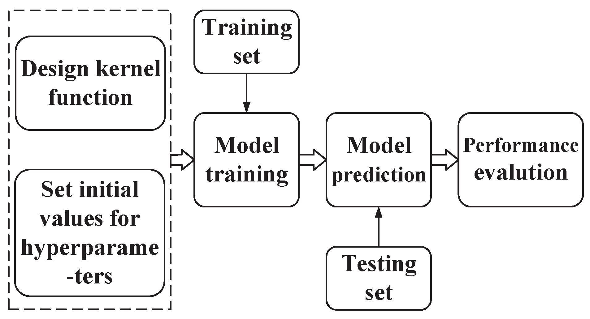
2.3. Establishment of GPR Models

When we use GPR to model the power and wavelength of the DBR laser, the training sets are selected as $\left\{I,T,P\right\}$ and $\left\{I,T,\lambda \right\}$, respectively. Then, we should focus on the design of the covariance kernel function, which is the key to the performance of the GPR model. According to the existing theory, there are several commonly used covariance kernel functions to choose from, such as the squared exponential covariance function, Matern covariance function, rational squared covariance function, and periodic covariance function. The covariance function needs to be set appropriately according to the characteristics of the data for accurate description. To achieve an accurate description of the DBR laser output power and wavelength, a suitable modification kernel that takes into account the physical properties of the laser is necessary.

We evaluate the influence of the current and temperature on the output power through Equation (4). It can be seen from the classical formula that the influence of the temperature and current on power mainly presents exponential and polynomial trends. Therefore, we designed the corresponding single covariance kernel functions separately according to these two effects. For the exponential part, we designed the corresponding kernel function $k_1$ as follows:

$$k_1\left(x_1,x_1^{\prime }\right)=l_1·exp\left(-\frac{1}{{\sigma }_1}∥\frac{1}{x_1}-\frac{1}{x_1^{\prime }}∥\right)$$

(14)

where $l_1$ and ${\sigma }_1$ are two hyperparameters of this kernel.

For the polynomial part, the corresponding kernel function $k_2$ was designed as follows:

$$k_2\left(x_2,x_2^{\prime }\right)={\left(l_2·x_2^T{x}_2^{\prime }+c\right)}^d$$

(15)

where the slope $l_2$, the constant term ${\sigma }_1$, and the polynomial degree d are the hyperparameters of this kernel.

GPR kernel functions must be positive and semi-definite, which means that most combinations of single-kernel functions are additions or simple multiplications. Considering that the current and temperature of the DBR laser have a strong correlation, we multiplied the above two single-kernel functions to generate a new combined kernel function to reflect the mutual influence of the input quantities. The combined kernel function was formulated as follows:

$$\begin{array}{c}{k}_{\mathrm{modified}1}\left(x,x^{\prime }\right)=l_1·exp\left(-\frac{1}{{\sigma }_1}∥\frac{1}{x_1}-\frac{1}{x_1^{\prime }}∥\right)·{\left(l_2·x_2^T{x}_2^{\prime }+c\right)}^d\end{array}$$

(16)

where x and $x^{\prime }$ denote the input vectors as $x=\left(x_1,x_2\right)$ and $l_1$, ${\sigma }_1$, $l_2$, c, and d are the corresponding hyperparameters. Theoretically, the DBR laser power can be described more accurately using this modified kernel.

For the output wavelength, there is no clear quantitative formula. According to the usual experience, we can easily find that the wavelength of the DBR laser changes in a linear trend with the current and temperature within a specific range. Considering that there will be a local nonlinear trend due to mode hopping, we designed the combined kernel function for the wavelength as follows:

$$k_{\mathrm{modified}2}\left(x,x^{\prime }\right)=\sum {\sigma }_2^{2}x{x}^{\prime }+{\sigma }_3^{2}exp\left[-\frac{2}{l_3^2}{sin}^2\left(\pi \right|x-x^{\prime }|/p)\right]$$

(17)

where ${\sigma }_2$, ${\sigma }_3$, $l_3$, and p are the corresponding hyperparameters. We added the linear kernel function and the periodic kernel function to obtain this new combined kernel function, which has an overall linear trend and can describe local nonlinear changes.

In order to improve the performance of the models, the hyperparameters of the covariance function need to be optimized in the training process. We chose the maximum likelihood estimation method to optimize the hyperparameters of the two combined kernel functions. First, the negative log-likelihood function $L\left(\theta \right)$ of the conditional probability of the training sample was established, and the partial derivative of the hyperparameter was obtained. Then, the optimal solution for the hyperparameter was obtained by minimizing the partial derivative using the conjugate gradient method. Here, the negative log-likelihood function $L\left(\theta \right)$ and its partial derivatives concerning the hyperparameters were in the form [39]

$$\left\{\begin{array}{c}L\left(\theta \right)=\frac{1}{2}log[det\lambda \left(\theta \right)]+\frac{1}{2}{y}^T{\lambda }^{-\mathbf{1}}\left(\theta \right)y+\frac{n}{2}log\left(2\pi \right)\\ \lambda \left(\theta \right)=k\left(\theta \right)+{\sigma }_n^2{I}_n\end{array}\right.$$

(18)

where $\theta$ represents the hyperparameters existing in the covariance function. The process of GPR model is shown in Figure 1.

3. Experiments and Result Analysis

3.1. Experimental Set-Up

In order to verify the effectiveness of the Gaussian process regression method proposed in this paper in solving the power and wavelength modeling problems of DBR lasers, we conducted corresponding experiments and data analysis. An experimental set-up was built for data acquisition. The laser was divided into two beams for power and wavelength measurement. The laser diode was a PH852DBR (Photodigm), and its threshold current was 50 mA. We used a wide range of high-performance current controllers to drive the laser diodes with a control accuracy of 2 µ$\mathrm{A}$. A temperature controller was used for real-time temperature measurement and control with an accuracy of $2\mathrm{mK}$. The power meter we used was a PM160 for power measurement with $\pm 3\%$ (451–1000 nm) accuracy. The wavelength of the laser was measured by a wavelength meter (High Finesse WS7-60), with an accuracy and resolution of $60\mathrm{MHz}$.

We used the established experimental set-up for data collection. After processing, the data were used in GPR modeling for training and validation. The experimental set-up and process are shown in Figure 2.

First, we turned the laser on at the usual operating point for several minutes to reach a steady state. Then, we changed the input amount separately and measured the output characteristics of the laser. During the measurement, the ambient temperature was constant. The current regulation range of this laser was 50–150 mA, and the temperature regulation range was 19–26 °C. Within this range, we individually changed the current and temperature values in fixed increments (the current increment was 1 mA, and the temperature increment was 0.2 °C), and the power and wavelength measurements were performed after waiting for a fixed steady state time. The two processes were repeated three times. It should be noted that the steady state waiting time for a temperature change was longer than that of the current for the hysteresis of temperature control.

The collected data were filtered with the $3\sigma$ principle. Since the scale of the data was not significant (to the order of hundreds), K-fold cross-validation was used to process the data set. In this method, all the data are divided into K parts. One will be chosen for testing without repetition, and the others will be used as the training set to train the model. Then, it will calculate the ${\mathrm{MSE}}_i$ of the model on the test set, and finally, all the obtained ${\mathrm{MSE}}_i$ are averaged as follows:

$${\mathrm{CV}}_{\left(k\right)}=\frac{1}{k}\sum _{i=1}^k{\mathrm{MSE}}_i$$

(19)

Compared with the conventional validation set method, this cross-validation method dramatically reduces the impact of the division method. According to careful consideration of the training effect and training volume, K was set to five here.

This study uses current and temperature as model inputs and power and wavelength as model outputs. In power modeling, we collected and selected 390 valid data points. Because of the choice of 5-fold cross-validation, the training set had 312 data points, and the test set had 78 data points in each model’s training and evaluation. We collected and selected 590 effective data points for wavelength modeling and applied 5-fold cross-validation. The training set in each model’s training and evaluation contained 472 data points, and the test set contained 118 data points. The specific details of GPR modeling are mentioned in Section 2.3. We trained the processed data with different covariance kernels for the laser power and wavelength.

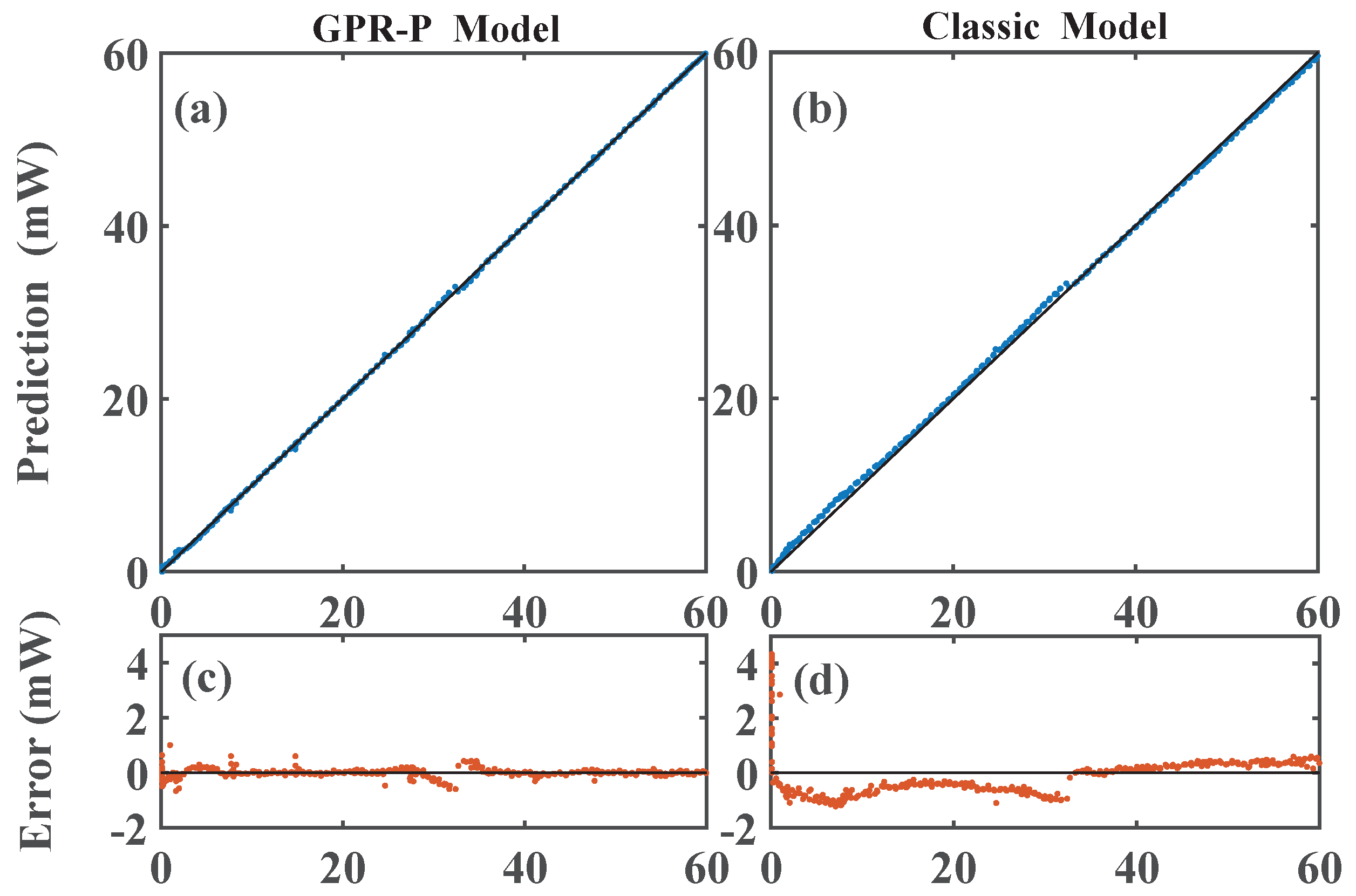
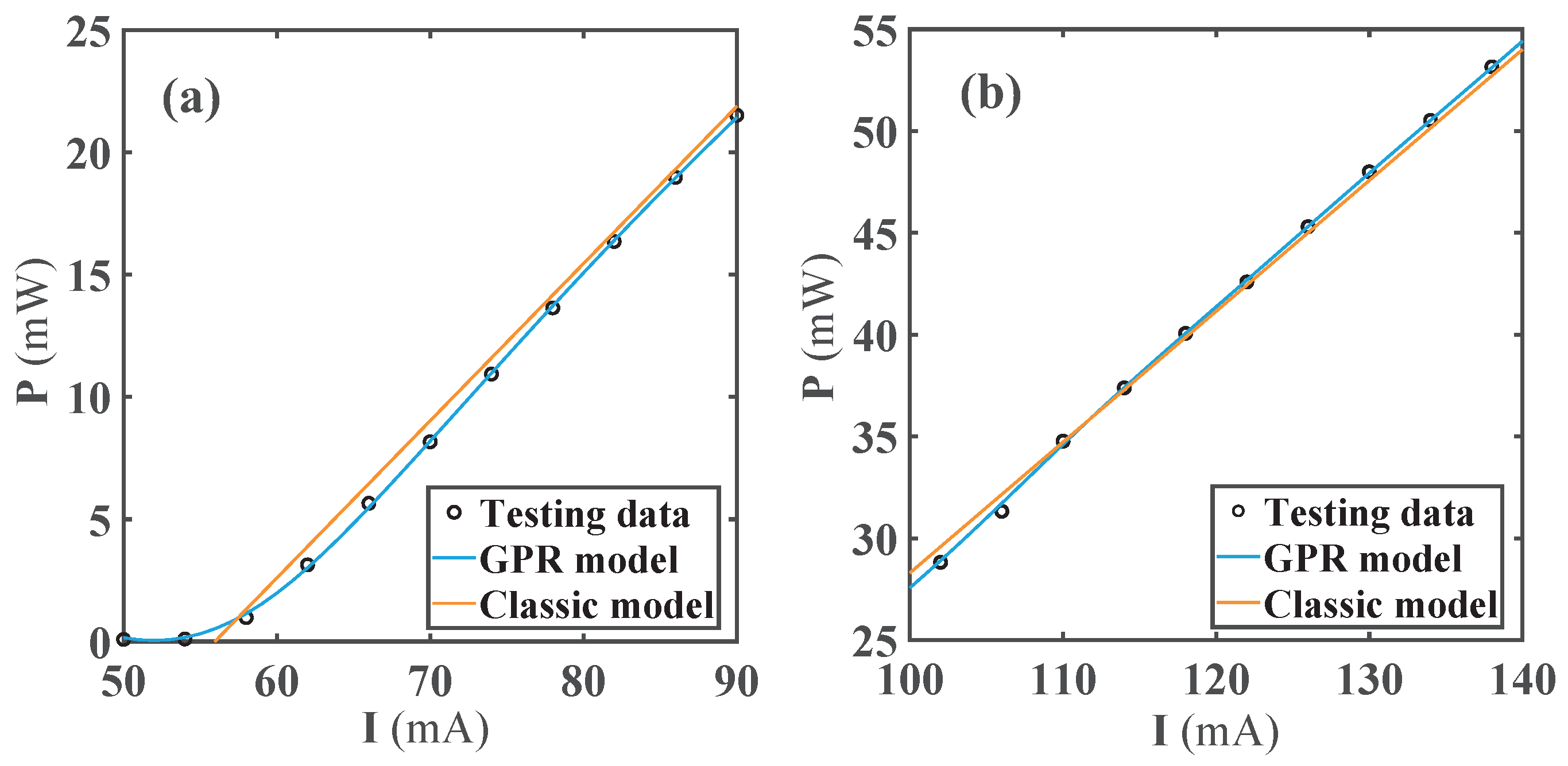
3.2. Model Validation

After the model design, data acquisition, and processing, we optimized the kernel parameters of GPR with the training set to achieve the optimal model. The previously proposed GPR−P and GPR−$\lambda$ models are validated and discussed in detail. In order to quantitatively analyze the accuracy of the model, two performance indicators are applied here:

(1) Root Mean Square Error (RMSE): The RMSE is the sample standard deviation of the difference between the predicted and observed values. It represents the discrete degree of the sample. In nonlinear fitting, the smaller the RMSE, the more accurate the results. This indicator is defined as

$$RMSE=\sqrt{\frac{1}{M}\sum _{i=1}^M{\left(y_i-{\widehat{y}}_i\right)}^2}$$

(20)

where M is the number of prediction values and $y_i$ and $y_i^2$ represent the observed values and predicted values, respectively.

(2) Mean Absolute Error (MAE): The MAE represents the mean of the absolute error between the predicted and observed values. It is a linear score where all individual differences are equally weighted on the mean. This indicator is defined as

$$MAE=\frac{1}{M}\sum _{i=1}^M\left|y_i-{\widehat{y}}_i\right|$$

(21)

The larger absolute values will be penalized by giving a greater weight to using the RMSE than the MAE.

Considering that a classic model of power previously existed, we will focus on the comparison of the model proposed in this paper with the classic power model. The GPR−P model and classic model are trained using identical sets, and the testing set was used to evaluate the performance of the models. Figure 3 illustrates the predictions and errors of the two models in the testing set. We noticed that the prediction and error performance of the GPR−P model was significantly better than the classic model. The RMSE and MAE of the GPR−P model were 0.16921 mW and 0.10779 mW, respectively. Moreover, these two indicators of the classic model were 1.0078 mW and 0.65246 mW, respectively. It can be seen that the RMSE of the GPR−P model was less than one-fifth of that of the classic model. In order to observe the difference between the two models more intuitively, we selected the current and power fitting of the two models at a specific temperature for comparison. Figure 4 shows the comparison of the classic model and the GPR model. The current and power in the classic model had a linear relationship. The comparison chart was divided into two ranges for illustration. In the threshold (50 mA) to 90 mA, the classic model was in poor agreement with the test value. Its linear characteristics could not be applied to the power near the threshold value, while the GPR−P model could better match the test data. As the current increased, the GPR−P model performed well from 90 mA to 140 mA. While the classic model could only fit the data in the range of 110–115 mA, there were certain deviations from the test set in other intervals. Further analysis showed that the classic model could not accurately describe the actual output power of the DBR laser, especially in an extensive current range. We confirmed that the GPR−P model could predict the power well near the threshold current and at high currents. This new model is pivotal in power control under different numerical requirements.

According to the GPR−P model, the laser power can be predicted under the current and temperature values when the laser tube usually works. The power prediction of the GPR−P model is shown in Figure 5. We could observe the laser output power for injection currents ranging from 50 mA to 150 mA and temperatures ranging from 22 °C to 26 °C. The prediction model showed that the DBR laser power was significantly affected by the current, and when the temperature remained constant, the power increased as the current rose. According to this model, the power showed a decreasing trend with the increase in temperature, but the nonlinear effect from the temperature was relatively weak. When the current was constant, it was hard to see the significant change in power with temperature in the figure. The properties exhibited by the predictive model were consistent with the actual measured data. The GPR−P model designed based on the DBR laser characteristics provided a more accurate way to describe the power, which would improve the performance of the DBR power control.

The relationship between the DBR laser output wavelength and the input current and temperature was described by the GPR−$\lambda$ model. As a way to model power, we used the training set to optimize the model’s parameters. Furthermore, the remaining test was set to test the model’s performance. The RMSE of the GPR−$\lambda$ model was $4\times {10}^{-4}$ nm. Mode hopping existed in the DBR laser. An accurate description of the position of the mode hopping point is essential for controlling the laser frequency. Figure 6 illustrates the wavelength change, with the current rising at a fixed temperature in the test results of the GPR−$\lambda$ model. It was observed that there was a mode hopping point in the change process for the current’s rise at a specific temperature, and the model provided a good fit for the data points near the abrupt change. It can be seen that the GPR−$\lambda$ model could accurately describe the output wavelength of the DBR laser.

Based on this model, a wavelength change in an extensive range of current and temperature variations would be determined, which could play an essential role in high-precision and high-efficiency control of the DBR laser frequency. We used the GPR−$\lambda$ model to predict the DBR laser for injection currents ranging from 80 mA to 140 mA and for temperatures ranging from 19 °C to 26 °C, as shown in Figure 7. In the continuous interval of the non-mode-hop point, there was a marked rise in the wavelength with the increase in temperature and current. The GPR−$\lambda$ model clearly described the mode hopping position of this DBR laser, which could help us avoid unstable points in laser wavelength control to achieve precise and efficient laser frequency control.

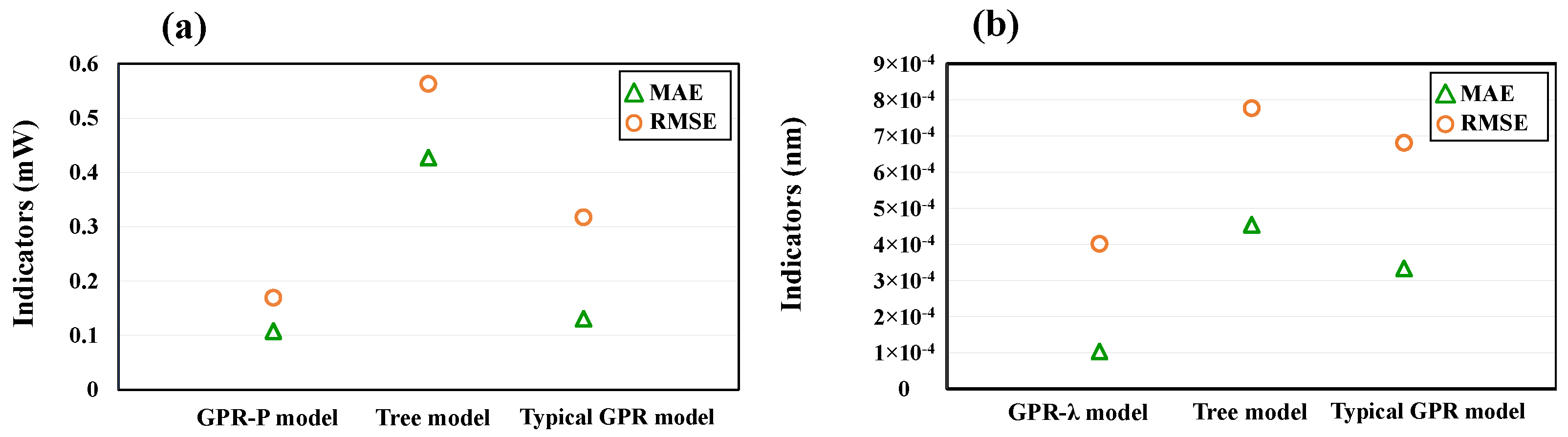
3.3. Discussion of the GPR Model’s Performance

To further evaluate the performance of the improved GPR power and wavelength models, another commonly used tree regression model in machine learning and a typical GPR model with an exponential kernel were trained based on the same dataset and compared with the improved GPR model proposed in this paper. The MAE and RMSE were chosen as quantitative measures of model performance. Figure 8 shows the performance of the improved GPR model, the tree regression model, and the typical GPR model on the power and wavelength data sets. The training results using the improved GPR model to describe the DBR laser output power and wavelength were better than those for the other two algorithms. Compared with the tree model, the MAE and RMSE of both GPR−P and GPR−$\lambda$ were significantly reduced, and additionally, both improved GPR models outperformed the typical GPR model.

The machine learning algorithm based on the Gaussian regression process can be better applied to model the power and wavelength of DBR lasers. We designed the kernel function of GPR based on the laser power and wavelength output characteristics for the first time. In the power modeling section, our power model explained the diode’s power more precisely than the classical power model. While improving the accuracy of power description, it also expanded the description range. In the wavelength modeling section, the RMSE of our wavelength model was roughly the same order of magnitude as the measurement error of commercial wavelength meters. This model fills a gap in previous studies on quantitative modeling of DBR laser wavelengths, providing a possibility to quantitatively describe the wavelengths of DBR lasers. In general, our GPR model saves a great deal of time while ensuring accuracy in modeling a distributed Bragg reflector laser’s power and wavelength. However, the GPR algorithm is computationally intensive. Further optimization of the description of the laser output characteristics in the future requires a specific design after weighing the model accuracy and computational cost.

4. Conclusions

In this paper, a machine learning method based on Gaussian process regression was proposed to describe the outpower and wavelength of a DBR laser. We developed and validated two improved GPR models (GPR−P model and GPR−$\lambda$ model) to determine the output power, wavelength, input current, and junction temperature, designing the appropriate kernel function and hyperparameters based on the physical mechanism of DBR lasers. The results show that our proposed GPR−P model could more accurately describe the power change of the diode from the current threshold to the maximum value compared with the classical power model, which could only describe the partial linear region of the power change. The RMSE of GPR−P was numerically less than one-fifth that of the classical power model. The RMSE of the GPR−$\lambda$ model proposed in this paper was $4\times {10}^{-4}$ nm, roughly the same order of magnitude as the measurement error of commercial wavelength meters, which provides a possibility to describe the wavelength of DBR lasers quantitatively. At the same time, this model’s accurate description of the nonlinear region is of great significance in avoiding the wavelength modulation point. This paper provides a convenient and precise method for the power and frequency control of DBR lasers. In the future, with continuous improvement of the kernel, it is expected to improve the accuracy and generality of the GPR model.

References

1. Wang, S. Principles of distributed feedback and distributed Bragg-reflector lasers. IEEE J. Quantum Electron. 1974, 10, 413. Available online: https://ieeexplore.ieee.org/abstract/document/1068152 (accessed on 2 February 2023).
2. Alexandrov, E.B.; Balabas, M.V.; Pasgalev, A.S.; Vershovskii, A.K.; Yakobson, N.N. Double-resonance atomic magnetometers: From gas discharge to laser pumping. Laser Phys. 1996, 6, 244. Available online: https://www.researchgate.net/publication/272183751_Double-resonance_atomic_magnetometers_From_gas_discharge_to_laser_pumping (accessed on 2 February 2023).
3. Tang, J.J.; Zhai, Y.Y.; Cao, L.; Zhang, Y.H.; Li, L.; Zhao, B.B.; Zhou, B.Q.; Han, B.C.; Liu, G. High-sensitivity operation of a single-beam atomic magnetometer for three-axis magnetic field measurement. Opt. Express 2021, 29, 15641. Available online: https://opg.optica.org/oe/fulltext.cfm?uri=oe-29-10-15641&id=450810 (accessed on 2 February 2023). [CrossRef] [PubMed]
4. Fang, J.C.; Qin, J. Advances in Atomic Gyroscopes: A View from Inertial Navigation Applications. Sensors 2012, 12, 6331. Available online: https://www.mdpi.com/1424-8220/12/5/6331 (accessed on 2 February 2023). [CrossRef]
5. Wang, Z.; Liu, S.X.; Wang, R.G.; Yuan, L.L.; Huang, J.; Zhai, Y.Y.; Zou, S. Atomic Spin Polarization Controllability Analysis: A Novel Controllability Determination Method for Spin-Exchange Relaxation-Free Co-Magnetometers. IEEE/CAA J. Autom. Sinica 2021, 9, 699. Available online: https://ieeexplore.ieee.org/abstract/document/9645928 (accessed on 2 February 2023). [CrossRef]
6. Zhai, Y.Y.; Yue, X.G.; Wu, Y.J.; Chen, X.Z.; Zhang, P.; Zhou, X.J. Effective preparation and collisional decay of atomic condensates in excited bands of an optical lattice. Phys. Rev. A 2013, 87, 063638. Available online: https://journals.aps.org/pra/abstract/10.1103/PhysRevA.87.063638 (accessed on 2 February 2023). [CrossRef]
7. Chen, X.; Yang, G.Q.; Wang, J.; Zhan, M.S. Coherent Population Trapping-Ramsey Interference in Cold Atoms. Chin. Phys. Lett. 2010, 27, 113201. Available online: https://iopscience.iop.org/article/10.1088/0256-307X/27/11/113201/meta (accessed on 2 February 2023).
8. Munoz, C. Dark matter detection in the light of recent experimental results. Int. J. Mod. Phys. A 2004, 19, 3093. Available online: https://www.worldscientific.com/doi/abs/10.1142/S0217751X04018154 (accessed on 2 February 2023). [CrossRef]
9. Stadnik, Y.V.; Flambaum, V.V. Enhanced effects of variation of the fundamental constants in laser interferometers and application to dark-matter detection. Phys. Rev. A 2016, 93, 063630. Available online: https://journals.aps.org/pra/abstract/10.1103/PhysRevA.93.063630 (accessed on 2 February 2023). [CrossRef]
10. Li, X.F.; Wang, Z.; Yu, L.; Ning, X.L.; Quan, W.; Zhai, Y.Y. Intelligent Modeling for Transfer Function Control of DBR Semiconductor Laser at Near-Working Point. IEEE Access 2020, 8, 24514. Available online: https://ieeexplore.ieee.org/abstract/document/8976149 (accessed on 2 February 2023). [CrossRef]
11. Kominis, K.I.; Kornack, T.W.; Allred, J.C.; Romalis, M.V. A subfemtotesla multichannel atomic magnetometer. New Test of Local Lorentz Invariance Using a Ne 21-Rb-K Comagnetometer. Nature 2003, 422, 596. Available online: https://www.nature.com/articles/nature01484 (accessed on 2 February 2023). [CrossRef] [PubMed]
12. Smiciklas, M.; Brown, J.M.; Cheuk, L.W.; Smullin, S.J.; Romalis, M.V. New Test of Local Lorentz Invariance Using a Ne21-Rb-K Comagnetometer. Phys. Rev. Lett. 2011, 107, 171604. Available online: https://journals.aps.org/prl/abstract/10.1103/PhysRevLett.107.171604 (accessed on 2 February 2023). [CrossRef] [PubMed]
13. Tang, J.J.; Yin, Y.; Zhai, Y.Y.; Zhou, B.Q.; Han, B.C.; Yang, H.Y.; Liu, G. Transient dynamics of atomic spin in the spin-exchange-relaxation-free regime. Opt. Express 2021, 29, 8333. Available online: https://opg.optica.org/oe/fulltext.cfm?uri=oe-29-6-8333&id=448763 (accessed on 2 February 2023). [CrossRef] [PubMed]
14. Yan, M.; Rickey, E.G.; Zhu, Y.F. Nonlinear absorption by quantum interference in cold atoms. Opt. Lett. 2001, 26, 548. Available online: https://opg.optica.org/ol/abstract.cfm?uri=ol-26-8-548 (accessed on 2 February 2023). [CrossRef]
15. Zhai, Y.Y.; Carson, C.H.; Henderson, V.A.; Griffin, P.F.; Riis, E.; Arnold, A.S. Talbot-enhanced, maximum-visibility imaging of condensate interference. Optica 2018, 5, 80. Available online: https://opg.optica.org/optica/fulltext.cfm?uri=optica-5-1-80&id=380874 (accessed on 2 February 2023). [CrossRef]
16. Kwee, P.; Willke, B.; Danzmann, K. Shot-noise-limited laser power stabilization with a high-power photodiode array. Opt. Lett. 2009, 34, 2912. Available online: https://opg.optica.org/ol/abstract.cfm?uri=ol-34-19-2912 (accessed on 2 February 2023). [CrossRef]
17. Shindo, Y. Application of polarized modulation technique in polymer science. Opt. Eng. 1995, 34, 3369. Available online: https://www.spiedigitallibrary.org/journals/optical-engineering/volume-34/issue-12/0000/Application-of-polarized-modulation-technique-in-polymer-science/10.1117/12.213252.short?SSO=1 (accessed on 2 February 2023). [CrossRef]
18. Budzyń, G.; Podżorny, T.; Tkaczyk, J. Method of improving the frequency repeatability of the intensity stabilized HeNe laser. Laser Phys. 2015, 25, 065002. Available online: https://iopscience.iop.org/article/10.1088/1054-660X/25/6/065002/meta (accessed on 2 February 2023).
19. Quan, W.; Li, Y.; Li, R.J.; Shang, H.N.; Fang, Z.S.; Qin, J.; Wan, S.A. Far off-resonance laser frequency stabilization using multipass cells in Faraday rotation spectroscopy. Appl. Opt. 2016, 55, 2503. Available online: https://opg.optica.org/ao/abstract.cfm?uri=ao-55-10-2503 (accessed on 2 February 2023). [CrossRef]
20. Liu, H.F.; Arahira, S.; Kunii, T.; Ogawa, Y. Tuning characteristics of monolithic passively mode-locked distributed Bragg reflector semiconductor lasers. IEEE J. Quantum Electron. 1996, 32, 1965. Available online: https://ieeexplore.ieee.org/abstract/document/541683 (accessed on 2 February 2023).
21. Demtröder, W. Laser Spectroscopy; Springer: Berlin/Heidelberg, Germany, 1982; p. 168. Available online: https://link.springer.com/book/10.1007/978-3-662-05155-9 (accessed on 2 February 2023).
22. Mahmood, A.; Irfan, A.; Wang, J.L. Machine learning for organic photovoltaic polymers: A minireview. Chin. J. Polym. Sci. 2022, 40, 870. Available online: https://link.springer.com/article/10.1007/s10118-022-2782-5 (accessed on 2 February 2023). [CrossRef]
23. Janjua, M.R.S.A.; Irfan, A.; Hussien, M.; Ali, M.; Saqib, M.; Sulaman, M. Machine-Learning Analysis of Small-Molecule Donors for Fullerene Based Organic Solar Cells. Energy Technol. 2022, 10, 2200019. Available online: https://onlinelibrary.wiley.com/doi/abs/10.1002/ente.202200019 (accessed on 2 February 2023). [CrossRef]
24. Mahmood, A.; Wang, J.L. A time and resource efficient machine learning assisted design of non-fullerene small molecule acceptors for P3HT-based organic solar cells and green solvent selection. J. Mater. Chem. A 2021, 9, 15684. Available online: https://pubs.rsc.org/en/content/articlelanding/2021/ta/d1ta04742f/unauth (accessed on 2 February 2023). [CrossRef]
25. Mebed, A.M.; Jafri, H.M.; Hakamy, A.; Abd-Elnaiem, A.M.; Sulaman, M.; Elshahat, S. Multidimensional modeling assisted mining of GDB17 chemical database: A search for polymer donors for organic solar cells and machine learning assisted performance prediction. Int. J. Quantum Chem. 2022, 122, 26991. Available online: https://onlinelibrary.wiley.com/doi/abs/10.1002/qua.26991 (accessed on 2 February 2023). [CrossRef]
26. Mahmood, A.; Irfan, A.; Wang, J.L. Developing efficient small molecule acceptors with sp2-hybridized nitrogen at different positions by density functional theory calculations, molecular dynamics simulations and machine learning. Chem.-Eur. J. 2022, 28, 202103712. Available online: https://chemistry-europe.onlinelibrary.wiley.com/doi/abs/10.1002/chem.202103712 (accessed on 2 February 2023). [CrossRef] [PubMed]
27. Mahmood, A.; Irfan, A.; Wang, J.L. Machine learning and molecular dynamics simulation-assisted evolutionary design and discovery pipeline to screen efficient small molecule acceptors for PTB7-Th-based organic solar cells with over 15% efficiency. J. Mater. Chem. A 2022, 10, 4170. Available online: https://pubs.rsc.org/en/content/articlehtml/2022/ta/d1ta09762h (accessed on 2 February 2023). [CrossRef]
28. Jordan, M.I.; Mitchell, T.M. Machine learning: Trends, perspectives, and prospects. Science 2015, 349, 255. Available online: https://www.science.org/doi/abs/10.1126/science.aaa8415 (accessed on 2 February 2023). [CrossRef]
29. Murata, N.; Yoshizawa, S.; Amari, S. Network information criterion-determining the number of hidden units for an artificial neural network model. IEEE Trans. Neural Netw. 1994, 5, 865. Available online: https://ieeexplore.ieee.org/abstract/document/329683 (accessed on 2 February 2023). [CrossRef]
30. Noble, W.S. What is a support vector machine? Nat. Biotechnol. 2006, 24, 1565. Available online: https://www.nature.com/articles/nbt1206-1565 (accessed on 2 February 2023). [CrossRef]
31. Schulz, E.; Speekenbrink, M.; Krause, A.A. tutorial on Gaussian process regression: Modelling, exploring, and exploiting functions. J. Math. Psychol. 2018, 85, 1. Available online: https://www.sciencedirect.com/science/article/abs/pii/S0022249617302158 (accessed on 2 February 2023). [CrossRef]
32. Nguyen-Tuong, D.; Seeger, M.; Peters, J. Model Learning with Local Gaussian Process Regression. Adv. Robotics 2009, 23, 2015. Available online: https://www.tandfonline.com/doi/abs/10.1163/016918609X12529286896877 (accessed on 2 February 2023). [CrossRef]
33. Quinonero-Candela, J.; Rasmussen, C.E. A Unifying View of Sparse Approximate Gaussian Process Regression. The J. Mach. Learn. Res. 2005, 6, 1939. Available online: https://www.jmlr.org/papers/volume6/quinonero-candela05a/quinonero-candela05a.pdf (accessed on 2 February 2023).
34. Zybin, A.; Koch, J.; Wizemann, H.D.; Franzke, J.; Niemax, K. Diode laser atomic absorption spectrometry. Spectrochimica Acta Part B At. Spectrosc. 2005, 60, 1. Available online: https://www.sciencedirect.com/science/article/abs/pii/S0584854704002794 (accessed on 2 February 2023). [CrossRef]
35. Pankove, J. Temperature dependence of emission efficiency and lasing threshold in laser diodes. IEEE J. Quantum Electron. 1968, 4, 119. Available online: https://ieeexplore.ieee.org/abstract/document/1075062 (accessed on 2 February 2023). [CrossRef]
36. O’donnell, K.P.; Chen, X. Temperature dependence of semiconductor band gaps. Appl. Phys. Lett. 1991, 58, 2924. Available online: https://aip.scitation.org/doi/abs/10.1063/1.104723 (accessed on 2 February 2023). [CrossRef]
37. Rasmussen, C.E.; Nickisch, H. Gaussian Processes for Machine Learning (GPML) Toolbox. The J. Mach. Learn. Res. 2010, 11, 3011. Available online: https://www.jmlr.org/papers/volume11/rasmussen10a/rasmussen10a.pdf?_hstc=200028081.1bb630f9cde2cb5f07430159d50a3c91.1524182400081.1524182400082.1524182400083.1_hssc=200028081.1.1524182400084_hsfp=1773666937 (accessed on 2 February 2023).
38. Yang, D.; Zhang, X.; Pan, R.; Wang, Y.J.; Chen, Z.H. A novel Gaussian process regression model for state-of-health estimation of lithium-ion battery using charging curve. J. Power Sources 2018, 384, 387. Available online: https://www.sciencedirect.com/science/article/abs/pii/S0378775318302398 (accessed on 2 February 2023). [CrossRef]
39. Seeger, M. Gaussian processes for machine learning. Int. J. Neural Syst. 2004, 14, 69. Available online: https://www.worldscientific.com/doi/abs/10.1142/S0129065704001899 (accessed on 2 February 2023). [CrossRef]
Figure 1. Process of GPR model.
Photonics 10 00193 g001
Figure 2. Experimental set-up.
Photonics 10 00193 g002
Figure 3. Predictions and errors for each point by the GPR−P model and classic model. (a) Predictions of the GPR−P model. (b) Errors of the GPR−P model. (c) Predictions of classic model. (d) Errors of the classic model.
Photonics 10 00193 g003
Figure 4. Comparison of the classic model and the GPR model for currents ranging from 50 mA to 140 mA. (a) Current ranging from 50 mA to 90 mA. (b) Current ranging from 100 mA to 140 mA.
Photonics 10 00193 g004
Figure 5. Power prediction of the GPR−P model.
Photonics 10 00193 g005
Figure 6. Change in wavelength with current rising at a fixed temperature in the test results for the GPR− λ model.
Photonics 10 00193 g006
Figure 7. Power prediction of the GPR−P model.
Photonics 10 00193 g007
Figure 8. Indicators of using different models in power and wavelength prediction. (a) Indicators in power prediction. (b) Indicators in wavelength prediction.
Photonics 10 00193 g008
Disclaimer/Publisher’s Note: The statements, opinions and data contained in all publications are solely those of the individual author(s) and contributor(s) and not of MDPI and/or the editor(s). MDPI and/or the editor(s) disclaim responsibility for any injury to people or property resulting from any ideas, methods, instructions or products referred to in the content.