The Block Landweber Iterative Method for Light Field Reconstruction from a Focal Stack

Abstract

Light field imaging involves reconstructing a 4D light field from a 3D focal stack, which makes it challenging to reconstruct the light field from incomplete projection data. To address this problem, a linear projection system is established to model the focal stack imaging process using discrete refocusing equations. Based on this system, we propose the block Landweber iterative method to find the least-squares solution. This method computes the sparse matrix while iterating, which overcomes the problem of data storage. The 2-norm of the block matrix is utilized as the weighted matrix to normalize every block matrix on an identical scale, delivering an effective relaxation strategy under the convergence condition in the inconsistent case, which yields better reconstruction results and accelerates the convergence speed. The experimental results based on the image quality assessments of reference and non-reference images show that our method achieved better reconstruction results compared to other relevant common methods, even with fewer focal stacks and higher angle resolution.

1. Introduction

The light field is a 4D function that captures the light rays entering a lens aperture. This encompasses not only the 2D projection information of the 3D scene that is acquired by traditional cameras but also records the 2D spatial and the 2D angular information [1,2]. The light field is regarded as a 2D array of images captured from various viewpoints, which are referred to as sub-aperture images. Due to the nature of the light field data, various post-capture image processing methods, including re-focusing [3], extended depth of field [4], depth estimation, and different viewpoint rendering [1], become more flexible. The applications of the light field make the acquisition of light field data very important. In order to record light field data, many acquisition methods have recently been designed such as light field data acquisition based on camera arrays [4]. However, this approach requires capturing multiple images using a cumbersome setup to obtain an adequate angular resolution. Additional optical elements can be integrated into the camera, such as microlens arrays [3], amplitude masks [5], coded apertures [6], and well-designed mirrors [7,8]. To create a unit picture, the light from the main lens passes through each microlens unit and onto a detector plane. Every point in the unit picture represents a beam of light that comes from the main lens (i.e., light field sampling). However, microlens arrays need to balance spatial and angular resolution, and the coded aperture may reduce the amount of light transmitted by the mask, resulting in insufficient brightness that affects image quality. There are drawbacks to both external lens and prism configurations, as well as heterodyne mask-enhanced cameras, including a loss of light and microdefects in the optical components.

Data collection based on the focal stack is one method, which involves an indirect way of acquiring a light field [9], wherein the light field is reconstructed by calculating collected images. Compared to the light field acquisition equipment of camera arrays, the data are collected using a typical digital camera, which has the advantage of being a lower-cost approach. In contrast to the microlens array and the coding mask of a light field camera, the spatial resolution of the focal stack data is sufficient, and some reconstruction algorithms can be used to reconstruct the light field at any angular resolution. In addition, the focal stack does not require the insertion of new optical devices.

The 3D focal stack can be used to reconstruct the 4D light field. By moving the lens or detector, the focal stack collects a series of images focused on several imaging planes. The set of captured images at different focal points is called the focal stack of the scene. Focal stack imaging has gained considerable attention in recent years [10], with researchers exploring various approaches to reconstruct the light field from the focal stacks. Alonso et al. [9] presented a method for refocusing with apertures of variable shapes and sizes from an optimal multi-focus image stack and for post-capture perspective shift reconstruction of a 3D scene. However, the results might not be reasonable if the sparse planes were unable to accurately convey the object scene. Tomographic reconstruction of epipolar images was accomplished by Mousnier et al. [11] by applying a masked back-projection approach, which involved calculating the focus and depth maps from the focal stack. Takahashi et al. [12] introduced a unique tensor light field display that could replace several focal stacks. However, this model can only use the same amount of focused images as the amount of layers of the tensor display. In order to render the 4D light field spectrum from all shifted 3D focal stack sequences, Levin and Durand [13] designed a linear view synthesis method by using a new light field prior in which the spectra of all shifted focal stack images are averaged and deconvolved by applying a slope-invariant kernel. However, the range of slopes of the focal stack required to build a slope-invariant kernel is much larger than the scene object; thus, this approach was unable to provide good results when sampling with limited slopes.

The algebraic iterative method is an effective method for reconstruction by discretizing the continuous light field into the form of a linear system. However, due to the large dimensions of the discrete matrices, storing these matrices takes up a lot of computer memory, leading to problems such as very slow convergence when iterative computations are performed. Yin et al. [14] proposed an iterative method that uses the guided filter to implement residual filtering during each sub-iteration, thereby reconstructing the 4D light field from the focal stack. Liu et al. [15] illustrated the importance of the object-image space consistency of focal stack-based light field reconstruction. However, the linear system is mostly inconsistent due to the influence of noise. Also, neither of these papers considered the influence of the relaxation coefficient. The quality of the reconstructed image is significantly influenced by the convergence condition and the selection of the relaxation coefficient. A unified framework for the convergence of simultaneous and block-iterative algorithms in consistent and inconsistent cases was proposed by Jiang and Wang [16]. Liu and Qu [17] proposed a refined iterative representation of the block Landweber method and found the optimal as well as the accelerated relaxation coefficients in the consistent case. The convergence strategy established in [17] can be utilized for light field reconstruction to obtain better reconstruction results.

In this paper, we propose the block Landweber iterative method to reconstruct the 4D light field from the 3D focal stack. Light field reconstruction is a serious ill-posed problem with incomplete projection data. The block Landweber iterative method [18] involves decomposing the linear system into blocks of equations, in which each block matrix represents a slice of each focal stack. Each block is subsequently treated using the Landweber method, and the least-square solution is found by iterating over all blocks cyclically. This block-by-slice approach of computing the sparse block matrix while iterating can effectively address data storage limitations when working with memory-constrained computers. The quality of the reconstructed image is influenced by the choice of the relaxation coefficient, which also has an impact on the computational stability and convergence behavior of the iterative method. The simultaneous iterative algorithm is the process of combining block matrices to solve large linear equations. The maximum eigenvalue of the global projection matrix determines the selection of the effective relaxation coefficient for the simultaneous iterative algorithm [19]. However, obtaining the global projection matrix poses a challenge due to insufficient storage. The linear system is usually inconsistent due to the influence of noise. Our primary objective is to establish effective relaxation strategies for a common block-iterative method based on the Landweber method under the convergence condition in inconsistent cases. If the relaxation coefficient satisfies the convergence condition, the iterative solution obtained using our method converges to the sum of a minimal 2-norm solution and the projection of the initial value onto the null space. The effective selection and adjustment of the relaxation coefficient satisfying the convergence condition results in appropriate improvements in reconstruction quality. Therefore, we use the integral imaging principle to construct an equation for discrete light field refocusing. The linear equations of different blocks are obtained by discretizing each slice of the focal stacks. In order to find an effective relaxation strategy under the convergence condition, the 2-norm of block matrices is used to build a weighted block matrix, and then each block matrix is normalized at an identical scale. Remarkably, satisfactory reconstruction of the light field is achieved even with a reduced amount of images captured from different focal points.

The remaining sections of the paper are organized as follows. The continuous and discrete forms of the refocusing equation are presented in Section 2. In Section 3, the block Landweber iterative method is proposed to reconstruct the light field from the focal stack, and the convergence results and corresponding relaxation strategy are presented. Section 4 presents some experimental results, followed by the discussions and conclusions in Section 5 and Section 6, respectively.

2. Light Field Reconstruction Based on the Focal Stack

In this section, we focus on a spatial-domain analysis, which directly connects the light field and the focal stack. We present the continuous and discrete forms of the focal stack transforms, respectively.

2.1. Continuous Focal Stack Transform

To parameterize the 4D light field $L(x, y, u, v)$, consider that all light rays proceed along the route from left to right, crossing through two parallel planes. In Figure 1, the light ray intersects the main lens plane at $(u, v)$, which determines the directional dimension of the ray. This light ray keeps moving and intersects the sensor plane at $(x, y)$, which represents the spatial dimension. According to traditional radiometry, the irradiance of a point on the imaging plane is equal to the weighted integral of the radiance of all the light rays passing through the lens and arriving at this point [3]. Assume that the light field $L(x, y, u, v)$ is compactly supported, $\mathrm{supp}\left(L\right)\subset D_1\times D_2$,

$$D_1=\left\{(x,y)\right|\left|x\right|\le {\widehat{d}}_1,\left|y\right|\le {\check{d}}_1\},D_2=\left\{(u,v)\right|u^2+v^2<d_2^2\},\Omega =D_1\times D_2,$$

(1)

where ${\widehat{d}}_1$ and ${\check{d}}_1$ are half-sizes corresponding to the x- and y-dimensions of the image, and $d_2$ is the radius of the aperture. Let the focal stack be $E_{{\rho }_m}(x_{{\rho }_m},y_{{\rho }_m})$, where ${\rho }_m=1-{\alpha }_m$, ${\alpha }_m=\frac{F_m}{F}$, and F is the distance between the $uv$ plane and the sensor plane. If the sensor plane is positioned inside the camera at any distance $F_m$, the light field focused on the new sensor plane at $F_m={\alpha }_m·F$ is as follows [3]

$$E_{{\rho }_m}(x_{{\rho }_m},y_{{\rho }_m})=\underset{D_2}{\int \int }L(x_{{\rho }_m}-{\rho }_{m}u,y_{{\rho }_m}-{\rho }_{m}v,u,v)dudv,$$

(2)

where ${\rho }_m={\rho }_1,\cdots ,{\rho }_M$ is obtained from a collection of images captured at different focal points.

2.2. Discrete Focal Stack Transform

The continuous light field function $L(x, y, u, v)$ is compactly supported in Equation (1). $\Omega$ can be partitioned into a hypercube grid with dimensions of $N_x\times N_y\times N_u\times N_v$. According to Equation (2), the focal stack $E_{{\rho }_m}$ is known for focal distances $F_m$ with $m=1,\cdots ,M\in \mathbb{Z}$. The aim of light field reconstruction is to find the approximate light field $L(x, y, u, v)$ by solving the discrete form of the reconstruction Equation (2). As the number of ${\rho }_m$ increases, the image reconstruction results will improve. The focal stack $E_{{\rho }_m}$ is known at points $(x_{{\rho }_m},y_{{\rho }_m})=(t_1\Delta x,t_2\Delta x)$ with $t_1=-n_x,\cdots ,n_x\in \mathbb{Z}$ and $t_2=-n_y,\cdots ,n_y\in \mathbb{Z}$, which satisfy $|t_1\Delta x|<{\widehat{d}}_1,|t_2\Delta x|<{\check{d}}_1$. By taking these known points $(t_1\Delta x,t_2\Delta x)$ of $E_{{\rho }_m}$, the discrete form of Equation (2) is

$$E_{{\rho }_m}(t_1\Delta x,t_2\Delta x)={(\Delta u)}^2\sum _{i=-n_u}^{n_u}\sum _{j=-n_v}^{n_v}L\left(t_1\Delta x-i{\rho }_m\Delta u,t_2\Delta x-j{\rho }_m\Delta u,i\Delta u,j\Delta u\right).$$

(3)

Since $L(x, y, u, v)$ has a compact support $\mathrm{supp}\left(L\right)\subset \Omega$, the variables x, y, u, and v are discretized at equal grids, $x=p\Delta x$, $y=q\Delta x$, $u=i\Delta u$, and $v=j\Delta u$, where $p=-n_x,\cdots ,n_x\in \mathbb{Z}$, $q=-n_y,\cdots ,n_y\in \mathbb{Z}$, $i=-n_u,\cdots ,n_u\in \mathbb{Z}$, $j=-n_v,\cdots ,n_v\in \mathbb{Z}$, satisfying $|p\Delta x|\le {\widehat{d}}_1$, $|q\Delta x|\le {\check{d}}_1$, $|i\Delta u|\le d_2$, and $|j\Delta v|\le d_2$. In general, $t_1\Delta x-i{\rho }_m\Delta u$ and $t_2\Delta x-j{\rho }_m\Delta u$ are not equal grids in Equation (3). $L\left(t_1\Delta x-i{\rho }_m\Delta u,t_2\Delta x-j{\rho }_m\Delta u,i\Delta u,j\Delta u\right)$ is estimated using $L(p\Delta x,q\Delta x,i\Delta u,j\Delta u)$, with bilinear interpolation at these discrete points $x_{{\rho }_m}=t_1\Delta x$, $y_{{\rho }_m}=t_2\Delta x$, $u=i\Delta u$, and $v=j\Delta u$. In order to facilitate the calculation, $\Delta u=S\Delta x$ is unified into units. Let $\Delta x=\Delta$, and then $\Delta u=S\Delta x=S\Delta$. Equation (3) is subsequently written as

$$E_{{\rho }_m}(t_1\Delta ,t_2\Delta )=S^2{\Delta }^2\sum _{i=-n_u}^{n_u}\sum _{j=-n_v}^{n_v}L\left((t_1-i{\rho }_{m}S)\Delta ,(t_2-j{\rho }_{m}S)\Delta ,iS\Delta ,jS\Delta \right).$$

(4)

Suppose that [20]

$$t_1\Delta -i{\rho }_{m}S\Delta =(m_0+a_0)\Delta ,t_2\Delta -j{\rho }_{m}S\Delta =(n_0+b_0)\Delta ,$$

(5)

where $m_0$, $n_0$ are integers, and $0\le a_0<1$, $0\le b_0<1$. Thus, using bilinear interpolation,

$$\begin{array}{cc}L\left(t_1\Delta -i{\rho }_{m}S\Delta ,t_2\Delta -j{\rho }_{m}S\Delta ,iS\Delta ,jS\Delta \right)\hfill & \\ =\left(1-a_0\right)\left(1-b_0\right)L\left(m_0\Delta ,n_0\Delta ,iS\Delta ,jS\Delta \right)+a_0\left(1-b_0\right)L\left(\left(m_0+1\right)\Delta ,n_0\Delta ,iS\Delta ,jS\Delta \right)\hfill & \\ +\left(1-a_0\right)b_{0}L\left(m_0\Delta ,\left(n_0+1\right)\Delta ,iS\Delta ,jS\Delta \right)+a_0{b}_{0}L\left(\left(m_0+1\right)\Delta ,\left(n_0+1\right)\Delta ,iS\Delta ,jS\Delta \right).\hfill \end{array}$$

(6)

For notational simplicity, $E_{{\rho }_m}(t_1\Delta ,t_2\Delta )$ and $L(p\Delta ,q\Delta ,iS\Delta ,jS\Delta )$ are replaced with ${\overline{E}}_{{\rho }_m}(t_1,t_2)$ and $\overline{L}(p,q,i,j)$, respectively. For each ${\rho }_m$, we have

$$\begin{array}{cc}\hfill {\overline{E}}_{{\rho }_m}(t_1,t_2)& =\sum _{p=-n_x}^{n_x}\sum _{q=-n_y}^{n_y}\sum _{i=-n_u}^{n_u}\sum _{j=-n_v}^{n_v}{A}_m(t_1, t_2; p, q, i, j)\overline{L}(p, q, i, j)\hfill \\ \hfill & =\sum _{p=m_0}^{m_0+1}\sum _{q=n_0}^{n_0+1}\sum _{i=-n_u}^{n_u}\sum _{j=-n_v}^{n_v}{A}_m(t_1, t_2; p, q, i, j)\overline{L}(p, q, i, j),\hfill \end{array}$$

(7)

where $p=\{m_0,(m_0+1)\}$, $q=\{n_0,(n_0+1)\}$, $A_m$ is the projection matrix. Equation (4) is a discrete refocusing equation that concatenates the sub-aperture images at the reference location F and the focal stack image focused at position $F_m$. It is derived from the integral imaging principle. Equation (7) is obtained using bilinear interpolation by substituting Equation (5) into Equation (6). Suppose that each slice of the focal stack has dimensions of $N_x\times N_y$. For the known focal stack $E_{{\rho }_m}$, in order to reconstruct the 4D light field L, vectorization calculation is performed according to Equation (7). If L is rewritten as a 1D vector, the dimensions of L are $(N_x\times N_y\times N_u\times N_v)\times 1$ and the dimensions of $E_{{\rho }_m}$ are $(N_x\times N_y)\times 1$. Then, $A_m$ is written in the form of a 2D matrix. Therefore, the projection matrix $A_m$ has dimensions of $P\times Q=(N_x\times N_y)\times (N_x\times N_y\times N_u\times N_v)$, $P=1,\cdots ,(2n_x+1)\times (2n_y+1)\in \mathbb{Z}$, $Q=1,\cdots ,(2n_x+1)\times (2n_y+1)\times (2n_u+1)\times (2n_v+1)\in \mathbb{Z}$. When $t_1,t_2,p,q,i,j$ take different values, for each ${\rho }_m={\rho }_1,\cdots ,{\rho }_M$, the positions of the elements in matrix ${\overline{E}}_{{\rho }_m}(t_1,t_2)$ and $\overline{L}(p,q,i,j)$ are determined by the following equation:

$$\begin{array}{cc}\hfill \overline{m}& =(t_1+n_x)(2n_y+1)+(t_2+n_y+1),\hfill \\ \hfill \overline{n}& =(i+n_u)(2n_v+1)(2n_x+1)(2n_y+1)+(j+n_v)(2n_x+1)(2n_y+1)\hfill \\ \hfill & +(p+n_x)(2n_y+1)+(q+n_y+1),\hfill \end{array}$$

(8)

where $\overline{m}$ and $\overline{n}$ are the positions of the number of rows and columns of matrix $A_m$, respectively. Then, matrix $A_m$ is obtained using Equation (4) through the bilinear interpolation of Equation (6). According to Equation (6), there are at most $4\times (2n_u+1)\times (2n_v+1)$ elements for each row of the matrix $A_m$, and the other values are all zero; thus, $A_m$ is sparse. Therefore, matrix $A_m$ is stored using sparse storage, which greatly reduces the amount of memory required and makes the calculation possible.

3. Iterative Scheme

In this section, based on the discrete focal stack transform, we establish the block Landweber iterative method to solve the linear system and the corresponding effective relaxation strategy.

3.1. Method

The value of $E_{{\rho }_m}$ at the pixel $(x_{{\rho }_m},y_{{\rho }_m})$ is equivalent to the integral of L for multiple viewpoints. For sub-aperture images, L from multiple viewpoints is obtained through the known focal stack $E_m$ and the corresponding projection matrix $A_m$, with $m=1,\cdots ,M\in \mathbb{Z}$. Thus, the M system of linear equations is obtained, combining the M system of linear equations to obtain a larger system of linear equations. That is, by assuming that the focal stack contains M slices, the linear system can be written as

$$Ax=b,$$

(9)

where $A={[A_1,\dots ,A_M]}^{\top }$ is the projection matrix. $x={[L^1,\dots ,L^N]}^{\top }$, $L^n$ is treated as one sample of the light field (a sub-aperture image), $b={[E_{{\rho }_1},\dots ,E_{{\rho }_M}]}^{\top }$. M is the number of captured images at different focal points, and the m-th slice of the stack corresponds to each sub-matrix $A_m$. A light field (sub-aperture images) can be projected onto a set of images focused at various depths by matrix A. The 4D light field x is reconstructed using the 3D focal stack b, and the discrete Equation (4) is used to solve the linear system (9) for light field reconstruction.

3.2. The Block Landweber Iterative Method

In this subsection, we introduce the block Landweber iterative method to reconstruct the light field from the focal stack. Suppose that the light field has angular dimensions of $N_u\times N_v$, spatial dimensions of $N_x\times N_y$, and M is the total number of slices in the focal stacks. The dimensions of matrix A are determined by $(M\times N_x\times N_y)\times (N_u\times N_v\times N_x\times N_y)$. When the image pixels are large, the number of focal stacks is too high, or the light field with a higher angular resolution is reconstructed, that is, the dimensions are too large, a computer that does not have enough memory may face the problem of not being able to store matrix $A^{\top }A$, which is required by some algorithms. In this case, the importance of the block iteration is evident. As mentioned above, even the sparse storage method is used to store matrix A. However, when performing multiple iterations, the matrix multiplication causes the sparseness of the matrix to be weakened, resulting in the inability to perform storage calculations. If the block Landweber iterative method is used for calculation, the relevant sub-matrix $A_m$ is recalculated in each block iteration, so that the whole projecting matrix A does not have to be stored in memory. This block-by-slice approach of computing the sparse block matrix while iterating can address the issue of insufficient memory. Another significant advantage of using the block Landweber iterative method is that it can speed up convergence. The amount of non-zero eigenvalues in the block matrix $A_m^{\top }{A}_m$ is less than the amount of non-zero eigenvalues in the overall matrix $A^{\top }A$. This phenomenon causes the convergence speed of the block Landweber iterative method to be faster than the convergence speed of the overall iteration. Therefore, we consider using the block Landweber iterative method to solve the linear system (9).

Since the amount of focal stacks of M is less than the amount of viewpoints N, the linear system (9) is an ill-posed problem. Suppose that the dimensions of the projection matrix A are $(M\times P)\times Q$. Then, the block iterative scheme based on the Landweber method is [16]

$$x^{(k+1)}=x^{\left(k\right)}+{\lambda }_k{A}_{\left[k\right]}^{\top }(b_{\left[k\right]}-A_{\left[k\right]}{x}^{\left(k\right)}),k=0,1,\cdots ,$$

(10)

where the control sequence is cyclic, i.e., $\left[k\right]\triangleq k\left(\mathrm{mod}M\right)+1$. Equation (10) is written as the following inner-outer iterative scheme, so the block Landweber iterative method is

$$\begin{array}{c}\hfill \left\{\begin{array}{cc}\hfill x^{(k,1)}& =x^{\left(k\right)},\hfill \\ \hfill x^{(k,m+1)}& =x^{(k,m)}+{\lambda }_{k,m}{A}_m^{\top }(b_m-A_m{x}^{(k,m)}),\hfill \\ \hfill x^{(k+1)}& =x^{(k,M+1)},\hfill \end{array}\right.\end{array}$$

(11)

where the relaxation coefficient ${\lambda }_{k,m}$ is different for each block iteration.

If matrix A is not partitioned, that is, matrix A is introduced into the computation as a whole, the block Landweber iteration is equivalent to the following Landweber iterative scheme [21]

$$x^{(k+1)}=x^{\left(k\right)}+{\overline{\lambda }}_k{A}^{\top }(b-A{x}^{\left(k\right)}),$$

(12)

where ${\overline{\lambda }}_k$ is the relaxation coefficient.

Due to the influence of noise, the linear system (9) is inconsistent. The block Landweber iterative scheme is a method for finding the least-square solutions of the linear system (9). The least-squares functional [19]

$$\left\{\begin{array}{cc}f\left(x\right)=\frac{1}{2}{\parallel b-Ax\parallel }^2\hfill & \\ minf\left(x\right)\hfill \end{array}\right.$$

(13)

is used to find the solution to Equation (9). All minimum points of $f\left(x\right)$ satisfy the normal equation

$$A^{\top }Ax=A^{\top }b.$$

(14)

Equation (14) is always solvable and has a minimal 2-norm solution $x^{+}$, which is equal to $A^{†}b$, where $A^{†}$ is the Moore–Penrose inverse of A [22]. When the linear system (9) is inconsistent, the constant vector b can be decomposed into $\overline{b}+\widehat{b}$, where $\overline{b}\in \mathcal{R}\left(A\right)$ and $\widehat{b}\in \mathcal{R}{\left(A\right)}^{\perp }$. According to the definition of the orthogonal complement, $\mathcal{R}{\left(A\right)}^{\perp }=\mathcal{N}\left(A^{\top }\right)$. Thus, when the linear system (9) is inconsistent, the following process is performed [23]

$$A^{\top }Ax=A^{\top }(\overline{b}+\widehat{b})=A^{\top }\overline{b}.$$

(15)

For the block Landweber iterative scheme (11), the limit is $x^{+}+P^A\left(x^0\right)$, which is also a solution to (14). $P^A\left(x^0\right)$ denotes an oblique projection of the initial value $x^{\left(0\right)}$ onto the null space $\mathcal{N}\left(A\right)$.

3.3. Convergence Results

For the Landweber iteration, regardless of whether the linear system (9) is consistent or inconsistent, the relaxation coefficient must satisfy the corresponding convergence condition.

Theorem 1

([24]). Let $\Vert A\Vert =\theta >0$. Assume that the relaxation coefficient is chosen such that $0\le {\overline{\lambda }}_k{\theta }^2\le 2$ for all $k\ge 0$. Thus, the iteration $x^{\left(k\right)}$ generated by the Landweber iteration Equation (12) converges to a solution to the normal Equation (14) if and only if

$$\sum _{k=0}^{\infty }{\gamma }_{1,k}=+\infty ,$$

(16)

where ${\gamma }_{1,k}=min({\overline{\lambda }}_k{\theta }^2,2-{\overline{\lambda }}_k{\theta }^2)$, and ${\theta }^2$ is the maximum eigenvalue of matrix $A^{\top }A$.

The following theorem provides the convergence condition in the inconsistent case for the proposed block Landweber iterative algorithm (10).

Theorem 2

([16]). Assume that there exists $a>0$ such that $\Vert A_m\Vert \le a$ for $m=1,\dots ,M$ and $0\le a^2{\lambda }_k\le 2$ for all $k\ge 0$. If subset $E_m$ is disjoint and even if the linear system (9) is inconsistent,

$$\underset{k\to \infty }{lim}{\lambda }_k=0\mathit{and}\sum _{k=0}^{\infty }{\lambda }_k=+\infty .$$

(17)

Under these conditions, the iteration $x^{\left(k\right)}$ generated by Equation (10) converges to $x^{+}+P^A\left(x^0\right)$.

3.4. The Relaxation Strategy

In this paper, we have assumed that the relaxation coefficient is not constant during one sub-iterative cycle, i.e., for each sub-matrix $A_m^{\top }{A}_m$, the relaxation coefficient ${\lambda }_{k,m}$ is a different value. In order to select an effective relaxation strategy to obtain better reconstruction results, the 2-norm of all sub-matrices $A_m$ are normalized for $m=1,\cdots ,M$ by dividing the second term on the right-hand side in Equation (11) by $\parallel A_m{\parallel }_2$, equivalent to ${\lambda }_{k,m}={\sigma }_k\frac{1}{\parallel A_m{\parallel }_2}$. Then, Equation (11) is transformed as

$$x^{(k,m+1)}=x^{(k,m)}+{\sigma }_k\frac{1}{\parallel A_m{\parallel }_2}{A}_m^{\top }(b_m-A_m{x}^{(k,m)}).$$

(18)

Note: for $M=1$, Equation (18) can be written in the form of the algebraic reconstruction technique (ART) iterative scheme:

$$x_{\overline{q}}^{(m+1)}=x_{\overline{q}}^{\left(m\right)}+\sigma \frac{b_{\overline{p}}-{\sum }_{\overline{k}=1}^Q{A}_{\overline{p}\overline{k}}{x}_{\overline{k}}^{\left(m\right)}}{{\sum }_{\overline{k}=1}^Q{A}_{\overline{p}\overline{k}}^2}{A}_{\overline{p}\overline{q}},\overline{p}=1,2,\cdots ,P,\overline{q}=1,2,\cdots ,Q.$$

(19)

Theorem 3

([17]). Suppose that $G_m=W_m^{\frac{1}{2}}{A}_m$, ${\overline{b}}_m=W_m^{\frac{1}{2}}{b}_m$, and the weighted block matrix is $W_m=\frac{1}{{\mu }_{1,m}}{I}_m$ for $m=1,\cdots ,M$, where ${\mu }_{1,m}$ is the maximum eigenvalue of $A_m^{\top }{A}_m$ and $I_m$ denotes the identity matrix of order P. Equation (18) is transformed as

$$x^{(k,m+1)}=x^{(k,m)}+{\sigma }_k{G}_m^{\top }({\overline{b}}_m-G_m{x}^{(k,m)}),$$

(20)

where ${\sigma }_k$ is the relaxation coefficient. If the linear system (9) is inconsistent, the iteration$x^{(k,m)}$generated by Equation (20) converges to $x^{+}+P^A\left(x^0\right)$ under the following conditions

$$\underset{k\to \infty }{lim}{\sigma }_k=0\mathit{and}\sum _{k=0}^{\infty }{\sigma }_k=+\infty .$$

(21)

Therefore, the relaxation coefficient ${\sigma }_k$ is assumed to be decreasing as the iteration times increase. There are many options for the sequence of ${\sigma }_k$ satisfying the convergence condition Equation (21). The following formulas are tested as the relaxation coefficient for the block Landweber iterative method (20),

$$\left(\mathrm{a}\right){\sigma }_k=\frac{\tau }{k+1},k=0,1,\cdots ,$$

(22)

$$\left(\mathrm{b}\right){\sigma }_k=\frac{\tau }{(k+1)\ast ln(k+3)},k=0,1,\cdots ,$$

(23)

where $\tau \in (0,1]$ is a parameter.

The harmonic series ${\sum }_{k=0}^{\infty }\frac{1}{k+1}=+\infty$ and ${lim}_{k\to \infty }\frac{1}{k+1}=0$. Then, option (a) of ${\sigma }_k$ satisfies the convergence condition Equation (21). For ${\sigma }_k=\frac{\tau }{(k+1)ln(k+3)}=\frac{\tau }{tln(t+2)}$, with $t=k+1$ monotonically decreasing, and suppose that $g\left(t\right)=\frac{1}{tln(t+2)}$, where g is a continuous, positive, decreasing function of t for all $t\ge 1$, ${lim}_{t\to \infty }g\left(t\right)=0$. Since ${\int }_k^{k+1}\frac{1}{tln(t+2)}dt<\frac{1}{kln(k+2)}$, ${\int }_1^{\infty }g\left(t\right)dt<{\sum }_{k=1}^{\infty }\frac{1}{kln(k+2)}$, and ${\int }_1^{\infty }\frac{1}{tln(t+2)}dt>{\int }_1^{\infty }\frac{1}{(t+2)ln(t+2)}dt={\int }_3^{\infty }{(lnz)}^{-1}d(lnz)=+\infty$. Therefore, option (b) of ${\sigma }_k$ satisfies the convergence condition Equation (21).

4. Experimental Results

In this section, we experimentally validate and discuss the effectiveness of our proposed method (20) under the convergence condition Equation (21). Several focal stacks from four datasets were tested:

• The 4D Light Field Benchmark dataset (‘Boxes’ and ‘Rosemary’ [25]) was generated by a computer (CVIA Konstanz & HCI Heidelberg) and has an angular resolution of $9\times 9$ and a spatial resolution of $512\times 512$.
• The INRIA Light field dataset contains light fields captured using a second-generation Lytro Illum camera (‘Lytro1GCamera’ and ‘Toys’ [26]), which has an angular resolution of $15\times 15$ and a spatial resolution of $625\times 434$.
• A first-generation Lytro camera was used to capture the ‘Fruits’ dataset [11].
• The real data were recorded using a Basler camera (Model: acA411220uc) with a Myutron prime lens (Model: HF5018V), an F-number of $f/1.6$, and a focal length of $f=25$ mm.

For the different datasets, a stack with a number of different slices was synthesized. The values of the light field data were normalized in the range of $[0, 1]$.

The Peak Signal-to-Noise Ratio (PSNR) and Structural Similarity Index Measure (SSIM) [27] evaluation methods, based on reference images, as well as the blind reference-less image spatial quality evaluator (BRISQUE) [28], natural image quality evaluator (NIQE) [29], and perception-based image quality evaluator (PIQE) [30] evaluation methods, based on non-reference images, were used to quantitatively evaluate the quality of the reconstructed images. The quality of the reconstructed images was higher, as these three no-reference quality metrics have lower scores. The PSNR value indicates the ability to suppress noise levels in the reconstructed results, where a higher PSNR value corresponds to less noise present in the image. The similarity between the original and reconstructed images was quantified by applying the SSIM. A high degree of resemblance is indicated by an SSIM score that is closer to 1. We compared our method to Levin’s method (also known as the linear view synthesis (LVS)) method, proposed in [13], and a guided filter-based iterative method (also known as the FI method), proposed in [14], to demonstrate the performance of our proposed method.

4.1. Simulation Data

The slices of 10 and 14 focal stacks were synthesized to evaluate our method for the ‘Boxes’ and ‘Rosemary’ experiments, respectively. The reconstruction accuracy is quantified by the SSIM and PSNR, and the convergence curve is presented in Figure 2. The provided SSIM and PSNR values were averaged over all sub-aperture images. As can be seen in Figure 2, compared to other methods, the block iteration method used fewer iterations to attain higher SSIM and PSNR values, and convergence was achieved more quickly.

Figure 3a,c show the focal stacks of the ‘Boxes’ and ‘Rosemary’ datasets, and Figure 3b,d show the relevant red and green wireframes highlighted in Figure 3a,c, respectively. Figure 4a displays the sketch maps of the viewpoint switching (sub-aperture images) connected with the reconstruction results of the block Landweber iterative method after six iterations. Figure 4b,c show the sub-aperture images of the central and boundary views of the reconstruction results obtained using our method, highlighted by the red and green wireframes in Figure 4a, and the error maps compared to the reference images, respectively.

4.1.1. Comparing Different Relaxation Coefficient Formulas

In this subsection, we compare the different formulas (a) and (b) for choosing the relaxation coefficient ${\sigma }_k$ proposed in Section 3.4, and verify that both Formulas (22) and (23) are effective when the relaxation coefficient satisfies the convergence condition (21). The relaxation coefficients for the ‘Boxes’ and ‘Rosemary’ experiments were set to $\tau =0.25$ and $\tau =0.2$ for $k=0,1,\cdots$.

Figure 5 shows the results of the convergence curve by selecting different formulas for ${\sigma }_k$ in the ‘Boxes’ and ‘Rosemary’ experiments. The ‘Boxes’ and ‘Rosemary’ experiments are represented in red and blue, respectively, and solid and dashed lines represent the relaxation coefficient Equation (22) and Equation (23) in (a) and (b), respectively. Since both (a) and (b) satisfy the convergence condition, we can see that regardless of the formula used, the curves of the PSNR and SSIM converge, so the relaxation coefficient Equation (22) is chosen for the calculations in the subsequent experiments.

4.1.2. Focal Stack Number

In this subsection, we discuss the effect of the number of captured images at different focal points for light field reconstruction. The relaxation coefficient for the ‘Boxes’ experiment was set to $\tau =0.25$ for $k=0,1,\cdots$. In the focal stack dataset, shown in Figure 3a, we selected 2 images (the first and last images), 5 images (selected at every interval of the total image), and 10 images as the captured images for light field reconstruction. The quantitative evaluation results comparing the different numbers of captured images at different focal points are depicted in

Table 1. Quantitative evaluation of the reconstructed light field with different numbers of focal stacks in the ‘Boxes’ experiment.

Method	Average SSIM and PSNR for All Views
	2		5		10
	SSIM	PSNR	SSIM	PSNR	SSIM	PSNR
LVS	0.7411	21.3103	0.7778	23.446	0.8458	25.2633
FI	0.4032	10.7146	0.7653	16.7028	0.8804	24.2654
Our method	0.7618	17.2243	0.9133	26.8554	0.9373	27.5334

. In the same scene range, a set of focal stack data needs to contain most of the information of the scene to obtain effective light field reconstruction results. The reconstruction results obtained are not usable when a significant amount of information is missing, such as when the input data consist of only two images. In addition, the error of the reconstructed light field decreases with the increase in the number of focal stacks.

4.1.3. Angular Resolution

The comparison experiments in other subsections of the light field reconstruction from the focal stack are based on a constant angular resolution (i.e., $u\times v=5\times 5$). The influence of the angular resolution on reconstructed light fields is covered in this subsection. The relaxation coefficients for the ’Boxes’ and ’Rosemary’ experiments are set to $\tau =[0.2, 0.25, 0.3]$ and $\tau =[0.15, 0.2, 0.25]$, with angular resolutions of $3\times 3$, $5\times 5$ and $7\times 7$. Furthermore, the central view images of the reconstructed light fields are exhibited and compared with the reference images.

Figure 6 shows the sub-aperture images from the central view corresponding to the three angular resolutions, respectively.

Table 2. Quantitative evaluation of the reconstructed light field with different angular resolutions.

Method	Average SSIM and PSNR for All Views
	$\mathbf{3}\times \mathbf{3}$		$\mathbf{5}\times \mathbf{5}$		$\mathbf{7}\times \mathbf{7}$
	Boxes
	SSIM	PSNR	SSIM	PSNR	SSIM	PSNR
LVS	0.8717	26.7195	0.8458	25.2633	0.8164	24.0324
FI	0.9122	27.2251	0.8804	24.2654	0.8635	22.3545
Our method	0.9183	27.4617	0.9385	27.4987	0.9491	27.0213
	Rosemary
	SSIM	PSNR	SSIM	PSNR	SSIM	PSNR
LVS	0.9008	26.7446	0.8799	25.4402	0.8488	24.2101
FI	0.9194	27.1431	0.9136	26.8578	0.9051	25.8106
Our method	0.9223	27.4177	0.9360	27.7976	0.9432	27.4324

presents the quantitative evaluation results comparing different methods with different angular resolutions. Furthermore, the errors of the reconstructed light field increase with the increase in the angular resolution in the FI and the LVS methods. The LVS approach was tested using the code provided by the authors of [13]. To obtain the best results, the PSF radius and maximum slope parameter in the algorithm were manually tweaked. Based on the various angular resolutions, the reconstruction results demonstrate that our method performed better than the other methods.

4.2. INRIA Dataset

The INRIA light field dataset was decoded using the Matlab Light Field Toolbox v0.5 [31,32]. Note that the toolbox was used to provide a 4D light field close to the raw images captured using a second-generation Lytro Illum camera. Lytro images are affected by vignetting and noise. We used the decoded images as the original images for comparison to verify the effectiveness of our method, which led to inaccuracies in the evaluation parameters. Therefore, quantitative evaluation parameters such as the SSIM and PSNR are not used in this subsection.

The focal stacks with 14 slices for the ‘Lytro1GCamera’ and 20 slices for the ‘Toys’ experiment were synthesized to evaluate our method, and the relaxation coefficient was set to $\tau =0.2$ for $k=1,2,\cdots$ in both experiments. The different viewpoints of the reconstructed images using the three methods are displayed in Figure 7 and compared to the reference images (Figure 7(a1,a2)).

As can be seen from the patch in Figure 7(b1,b2), the noise points of the original decoded images were eliminated using the block Landweber iterative method. The reconstructed images obtained using the FI method always contained some artifacts, as shown in Figure 7(c1,c2). In addition, there was a viewpoint offset between the central and outer views in the reconstructed results. A very evident viewpoint offset was also observed in the results of the LVS method, resulting in unclear images (the first and fifth columns in Figure 7(d1,d2)). The aberration at the edge part of the lens was typically greater than that at the central part of the lens, which may have been caused by lens distortion. However, despite the offset phenomenon in our method, the reconstructed images still exhibited good quality. In general, our method achieved good reconstruction results in this dataset.

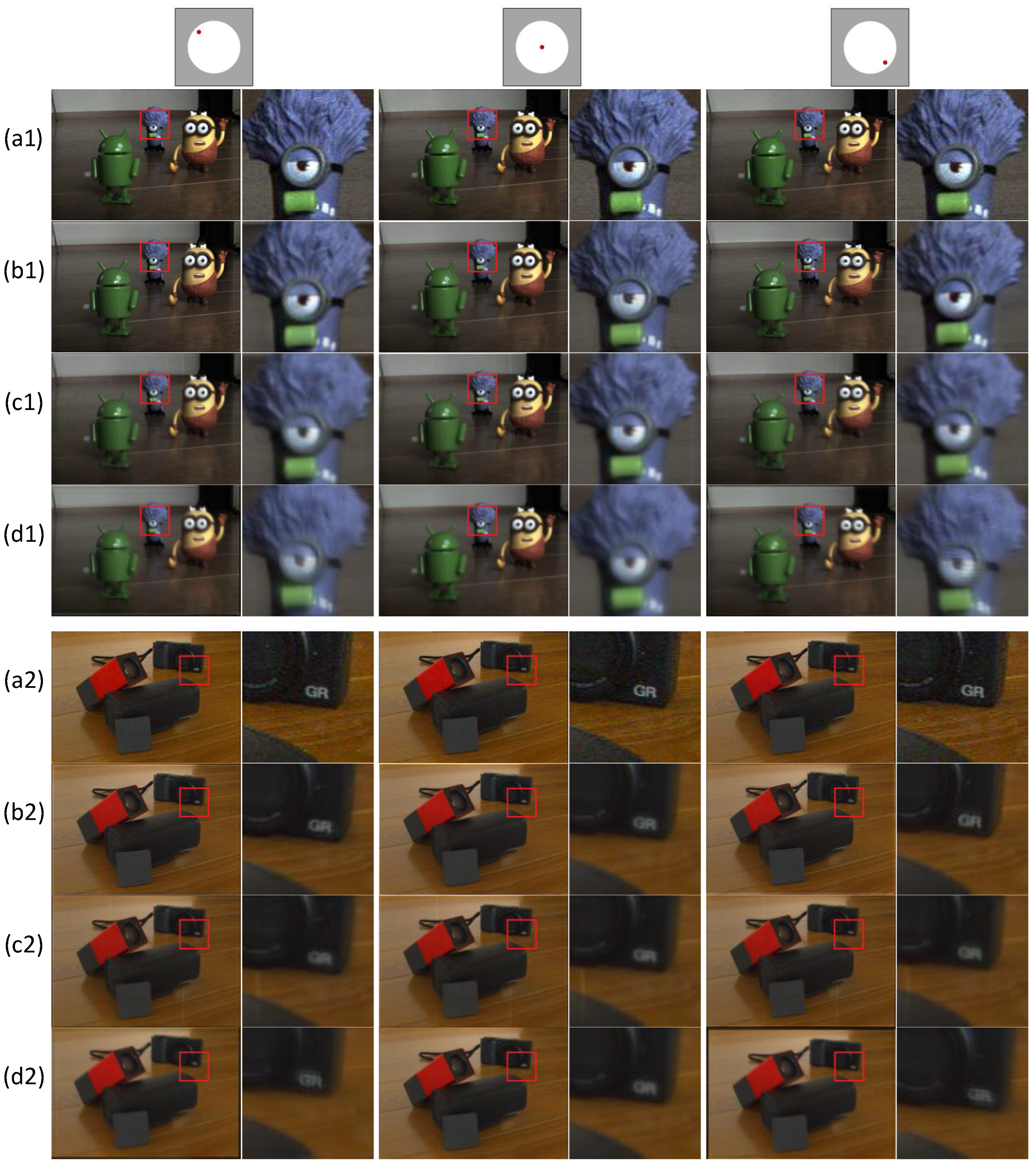
4.3. Real Focal Stack Data

Due to the lack of ground-truth data in the experiments using a first-generation Lytro camera and the real data, the BRISQUE, NIQE, and PIQE values were calculated to verify the reconstruction results of the experiments. The numbers of slices of the focal stacks were 12 and 16 for the ‘Fruits’ and ‘Pets’ experiments, with dimensions of $12\times 3\times 1088\times 1088$ and $16\times 3\times 981\times 594$, respectively. The relaxation coefficient was set to ${\sigma }_1=1$, $\tau =0.02$, $k=2,3,\cdots$ in both experiments.

Table 3. Quantitative evaluation of the reconstructed light field.

Method	Average SSIM and PSNR for All Views
	Fruits			Pets
	BRISQUE	NIQE	PIQE	BRISQUE	NIQE	PIQE
LVS	40.6613	4.4096	29.5531	39.8596	3.0506	56.662
FI	53.6426	4.3635	86.9005	46.574	4.4673	81.8001
Our method	10.033	3.1677	11.1459	25.6965	2.3513	39.3187

presents a comparison of the quantitative evaluation, showing that for the three indicators, our method performed the best in both experiments.

The reconstruction results and the close-up images of the local details shown in Figure 8 and Figure 9 demonstrate the effectiveness of our method. Since residual filtering was implemented using guided filters in each sub-iteration, as in [14], the error may increase in the reconstructed light field from the actual shot focal stack, leading to the artifacts shown in Figure 7c and Figure 9b. The reconstruction images of the synthetic light field data in Figure 6b do not exhibit this problem. Since the influence of the relaxation coefficient was not considered, although guided filtering was used in the FI method, our method yielded better reconstruction results compared to the FI method. Similar to the results in other datasets, the LVS model showed a significant viewpoint shift at the edge of the image. For the real data, such as the ‘Pets’ experiment, the results shown in Figure 8 reveal that our method yielded better reconstruction results compared to other methods, including the scale of the backboard and the details of the doll.

5. Discussion

This paper uses some image quality assessments based on reference and non-reference images to quantitatively evaluate the quality of reconstructed images in different datasets. The experimental results show that compared to the FI and LVS methods, our proposed method yields better reconstruction results. The quality of the reconstructed light field is related to the choice of the relaxation coefficient, the number of different focal point images captured, and the angular resolution. An experimental verification is conducted for the simulated dataset. It is possible to slightly improve the reconstruction results by choosing other relaxation coefficient formulas under convergence conditions. A small adjustment of the parameter $\tau$ in different datasets will also result in minor improvements in the reconstruction results. The number of captured focal stacks should be sufficient to contain most of the scene information for reconstructing effective light field images. Within the same scene range, increasing the number of focal stacks can achieve better reconstruction results. Compared to other methods, our method can obtain better reconstruction results, even when using fewer captured images at different focal points or when reconstructing light fields at higher angular resolutions.

6. Conclusions

In this paper, we have proposed a novel light field reconstruction algorithm, the block Landweber iterative method. The projection matrix is formed by concatenating the focal stack and the original light field views using bilinear interpolation. Each block matrix corresponds to a slice of the focal stack. The sparse block matrix $A_m$ is calculated per iteration and does not need to be stored, which overcomes the problem of data storage. Our block iterative approach has a wide variety of potential applications due to its computational efficiency and flexibility in terms of the number of input images. Our method is able to reconstruct high-quality light fields, even with a reduced amount of input data (a few images). According to the convergence conditions described in Section 3.3, the effective relaxation coefficient is necessary to obtain better reconstructed images. The 2-norm of the block matrix is utilized to construct the weighted matrix to normalize each block matrix on a unified scale, delivering effective relaxation strategies, as described in Section 3.4. The experimental results have shown that our method yields better reconstruction results compared to some corresponding methods.

References

1. Levoy, M.; Hanrahan, P. Light field rendering Aug. In Proceedings of the Siggraph96 Conference, New Orleans, LA, USA, 4–9 August 1996; pp. 31–42. [Google Scholar]
2. Gortler, S.J.; Grzeszczuk, R.; Szeliski, R.; Cohen, M.F. The Lumigraph. Proc. Siggraph. 1996, 96, 43–54. [Google Scholar]
3. Ng, R. Digital Light Field Photography. Ph.D. Thesis, Stanford University, Stanford, CA, USA, 2006. [Google Scholar]
4. Wilburn, B.; Joshi, N.; Vaish, V.; Talvala, E.V.; Antunez, E.; Barth, A.; Adams, A.; Horowitz, M.; Levoy, M. High performance imaging using large camera arrays. ACM Trans. Graph. 2005, 24, 765–776. [Google Scholar] [CrossRef]
5. Veeraraghavan, A.; Raskar, R.; Agrawal, A.K.; Mohan, A.; Tumblin, J. Dappled photography: Mask enhanced cameras for heterodyned light fields and coded aperture refocusing. ACM Trans. Graph. 2007, 26, 69. [Google Scholar] [CrossRef]
6. Levin, A. Image and Depth from a Conventional Camera with a Coded Aperture. In Proceedings of the SIGGRAPH2007, San Diego, CA, USA, 5–8 August 2007. [Google Scholar]
7. Fuchs, M.; Kächele, M.; Rusinkiewicz, S. Design and Fabrication of Faceted Mirror Arrays for Light Field Capture. Comput. Graph. Forum 2013, 32, 246–257. [Google Scholar] [CrossRef]
8. Manakov, A.; Restrepo, J.F.; Klehm, O.; Hegedüs, R.; Eisemann, E.; Seidel, H.P.; Ihrke, I. A Reconfigurable Camera Add-On for High Dynamic Range, Multispectral, Polarization, and Light-Field Imaging. ACM Trans. Graph. 2013, 32, 47. [Google Scholar] [CrossRef]
9. Alonso, J.R.; Fernández, A.; Ferrari, J.A. Reconstruction of perspective shifts and refocusing of a three-dimensional scene from a multi-focus image stack. Appl. Opt. 2016, 55, 2380. [Google Scholar] [CrossRef]
10. Lin, X.; Suo, J.; Wetzstein, G.; Dai, Q.; Raskar, R. Coded focal stack photography. In Proceedings of the IEEE International Conference on Computational Photography (ICCP), Cambridge, MA, USA, 19–21 April 2013; pp. 1–9. [Google Scholar] [CrossRef]
11. Mousnier, A.; Vural, E.; Guillemot, C. Partial light field tomographic reconstruction from a fixed-camera focal stack. arXiv 2015. Available online: http://www.irisa.fr/temics/demos/lightField/index.html (accessed on 17 March 2022). [CrossRef]
12. Takahashi, K.; Kobayashi, Y.; Fujii, T. From Focal Stack to Tensor Light-Field Display. IEEE Trans. Image Process. 2018, 27, 4571–4584. [Google Scholar] [CrossRef]
13. Levin, A.; Durand, F. Linear view synthesis using a dimensionality gap light field prior. In Proceedings of the 2010 IEEE Computer Society Conference on Computer Vision and Pattern Recognition, San Francisco, CA, USA, 13–18 June 2010; pp. 1831–1838. [Google Scholar] [CrossRef]
14. Yin, X.; Wang, G.; Li, W.; Liao, Q. Iteratively reconstructing 4D light fields from focal stacks. Appl. Opt. 2016, 55, 8457–8463. [Google Scholar] [CrossRef]
15. Liu, Y.; Zhang, R.; Feng, S.; Zuo, C.; Chen, Q.; Cai, Z. Consistency analysis of focal stack-based light field reconstruction. Opt. Lasers Eng. 2023, 165, 107539. [Google Scholar] [CrossRef]
16. Jiang, M.; Wang, G. Convergence Studies on Iterative Algorithms for Image Reconstruction. IEEE Trans. Med. Imaging 2003, 22, 569–579. [Google Scholar] [CrossRef]
17. Liu, Y.; Qu, G. Relaxation strategy for the block Landweber method. Phys. Scr. 2023, 98, 115217. [Google Scholar] [CrossRef]
18. Censor, Y.; Elfving, T. Block-Iterative Algorithms with Diagonally Scaled Oblique Projections for the Linear Feasibility Problem. SIAM J. Matrix Anal. Appl. 2002, 24, 40–58. [Google Scholar] [CrossRef]
19. Han, G.; Qu, G.; Jiang, M. Relaxation strategy for the Landweber method. Signal Process. 2016, 125, 87–96. [Google Scholar] [CrossRef]
20. Gao, S.; Qu, G. Filter-Based Landweber Iterative Method for Reconstructing the Light Field. IEEE Access 2020, 8, 138340–138349. [Google Scholar] [CrossRef]
21. Landweber, L. An iteration formula for fredholm integral equations of the first kind. Am. J. Math. 1951, 73, 615–624. [Google Scholar] [CrossRef]
22. Kirsch, A. An Introduction to the Mathematical Theory of Inverse Problems; Applied Mathematical Sciences; Springer: New York, NY, USA, 1996. [Google Scholar]
23. Han, G.; Qu, G.; Wang, Q. Weighting Algorithm and Relaxation Strategies of the Landweber Method for Image Reconstruction. Math. Probl. Eng. 2018, 2018, 5674647. [Google Scholar] [CrossRef]
24. Qu, G.; Wang, C.; Jiang, M. Necessary and Sufficient Convergence Conditions for Algebraic Image Reconstruction Algorithms. IEEE Trans. Image Process. 2009, 18, 435–440. [Google Scholar]
25. Honauer, K.; Johannsen, O.; Kondermann, D.; Goldluecke, B. A Dataset and Evaluation Methodology for Depth Estimation on 4D Light Fields. In Proceedings of the Computer Vision—ACCV 2016, Taipei, Taiwan, 20–24 November 2016; pp. 19–34. [Google Scholar] [CrossRef]
26. Jiang, X.; Le Pendu, M.; Farrugia, R.A.; Guillemot, C. Light Field Compression with Homography-Based Low-Rank Approximation. IEEE J. Sel. Top. Signal Process. 2017, 11, 1132–1145. Available online: https://www.irisa.fr/temics/demos/lightField/LowRank2/datasets/datasets.html (accessed on 17 March 2022). [CrossRef]
27. Zhou, W.; Bovik, A.C.; Sheikh, H.R.; Simoncelli, E.P. Image quality assessment: From error visibility to structural similarity. IEEE Trans Image Process. 2004, 13, 600–612. [Google Scholar]
28. Mittal, A.; Moorthy, A.K.; Bovik, A.C. No-Reference Image Quality Assessment in the Spatial Domain. IEEE Trans. Image Process. 2012, 21, 4695–4708. [Google Scholar] [CrossRef] [PubMed]
29. Mittal, A.; Soundararajan, R.; Bovik, A.C. Making a “Completely Blind” Image Quality Analyzer. IEEE Signal Process. Lett. 2013, 20, 209–212. [Google Scholar] [CrossRef]
30. Venkatanath, N.; Praneeth, D.; Bh, M.C.; Channappayya, S.S.; Medasani, S.S. Blind image quality evaluation using perception based features. In Proceedings of the 2015 Twenty First National Conference on Communications (NCC), Mumbai, India, 27 February–1 March 2015; pp. 1–6. [Google Scholar] [CrossRef]
31. Dansereau, D.G.; Pizarro, O.; Williams, S.B. Decoding, Calibration and Rectification for Lenselet-Based Plenoptic Cameras. In Proceedings of the IEEE Conference on Computer Vision & Pattern Recognition, Portland, OR, USA, 23–28 June 2013; pp. 1027–1034. Available online: https://au.mathworks.com/matlabcentral/fileexchange/75250-light-field-toolbox-v0-5 (accessed on 16 March 2022).
32. Dansereau, D.G.; Pizarro, O.; Williams, S.B. Linear Volumetric Focus for Light Field Cameras. ACM Trans. Graph. 2015, 34, 15. [Google Scholar] [CrossRef]
Figure 1. The diagram of the focal stack.
Photonics 10 01219 g001
Figure 2. Convergence curves for average SSIM and PSNR for all views.
Photonics 10 01219 g002
Figure 3. Synthesized focal stacks from the HCI light field dataset: (a,c) focal stacks of the ‘Boxes’ and ‘Rosemary’ datasets; (b,d) relevant red and green wireframes highlighted in (a,c), respectively.
Photonics 10 01219 g003
Figure 4. Viewpoint switching of the reconstructed light field: (a) sketch map of sub-aperture images using the block Landweber iterative method; (b,c) enlarged central and boundary sub-aperture images related to the red and green wireframes highlighted in (a), along with the corresponding reconstruction error maps.
Photonics 10 01219 g004
Figure 5. Convergence curves of the SSIM and PSNR, averaged for all views, obtained by selecting different formulas for σ k .
Photonics 10 01219 g005
Figure 6. The center viewpoint of the reconstructed light field with different angular resolutions ( u × v ): (a) our method, (b) FI method, (c) LVS method.
Photonics 10 01219 g006
Figure 7. Different viewpoints of the reconstructed light field in the INRIA dataset: (a) Ground truth, (b) our method, (c) FI method, (d) LVS method.
Photonics 10 01219 g007
Figure 8. Different viewpoints of the reconstructed light field in the real dataset: (a) our method, (b) FI method, (c) LVS method.
Photonics 10 01219 g008
Figure 9. Different viewpoints of the reconstructed light field in the ‘Fruits’ experiment: (a) our method, (b) FI method, (c) LVS method.
Photonics 10 01219 g009