Abstract
In this work, we construct a model of an asymmetrically coupled network of semiconductor chaotic lasers in order to recognize noisy digital images of digits 0–9, derived from different samples in the digital image sets 0–9 found within the MNIST dataset. Here, the lasers network consists of eight asymmetrically coupled semiconductor lasers. The chaotic lasers network is driven by the external inputs, which encode one noise digital image to be recognized. The outputs of the chaotic lasers network driven by a total of 40 samples from the digital image sets 0–9 are utilized as ten sets of reference signals. The output of the chaotic lasers network induced by one noisy digital image is used as a test signal. By judging the maximum of the correlations of the test signal with the ten sets of reference signals, all noisy digital images 0–9 can be recognized well under different noises. Moreover, we further explore the recognition rate for each noisy digital image under different noises and a fixed injection strength. It is found that all noisy digital images can be recognized well under a certain low injection strength. The recognition-rates of all noisy digital images can further decrease to a certain extent under higher noise and a fixed the injection strength. The injection strength has little influence on the recognition rate of one noise digital image target with lower noise. The recognition rate under higher noise maintains a higher value (more than 0.9) when the injection strength is smaller than a certain value, but for the larger injection strength, the recognition rate exhibits further decrease. The modeled chaotic lasers network can play the role of photonic accelerators for the recognition of the noisy digital images.
1. Introduction
Photonic accelerators provide fast and efficient information processing by using photonic technologies to overcome the limitations of integrated circuit density in semiconductor technologies, known as the end of Moor’s law [1,2]. Significantly, photonic accelerators have been demonstrated for certain dedicated information processing in machine learning, such as a deep neural network, and they are expected to contribute to artificial intelligence. Recently, principles and technologies of photonic accelerators have been proposed and demonstrated in applications, such as an artificial photonic neural network [3], optical pass gate logic [4], photonic reservoir computing (PRC) [5,6,7,8], a semiconductor laser dynamical system [9,10,11,12,13,14] and so on.
The asymmetric coupling semiconductor lasers network (ACSCLN), as an optical dynamical system, has potential application in photonic neuromorphic computing and can play a role similar to PRC for information processing. As is well known, a PRC consists of a network of artificial neurons with arbitrary connections that form an optical nonlinear dynamical system called a reservoir. Input data, as predictive targets, are passed to the photonic reservoir, which creates a higher-dimensional representation of the inputs and generates output signals. The training for supervised learning is performed only at the readout layer, whereas the connections between the neurons of the photonic reservoir are decided at the beginning and never change. Here, the scheme proposed by us is obviously different from the PRC. An interesting aspect of our scheme is that the ACSCLN can be considered a black box: one needs only to know the output corresponding to input forces, not the detailed dynamics of the network. Therefore, the ACSCLN provides significant simplification compared to traditional photonic neural networks, where the connections between neurons (virtual nodes) are difficult to change in real time.
Here, we take a critical step forward in the field of the ACSCLN by demonstrating a very general method to encode and process information. The main ideas are given as follows. As shown in Figure 1, the ACSCLN appears chaotic dynamic by an external injection, which encodes the digital image to be recognized and act as a driving force. The chaotic signals generated by the ACSCLN are encoded in the coupled strengths or injected strengths associated with these forces. Significantly, compared with the traditional PRC, our scheme does not need to train output weights using the linear least-squares method in offline computer or online complex photonic hardware system.
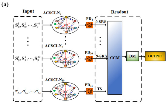
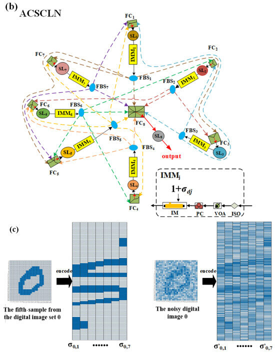
Figure 1.
(a) The system box diagram of the recognition pf the noisy digital images based on the photonic ACSCLN using the correlation calculations. (b) The detailed light paths of an ACSCLN, consisting of eight asymmetrically coupled SLs (acting as an ensemble of artificial neurons). Here, the ACSCLN with subscript of d is driven by the external inputs (, , …,), respectively, which are from the feature vectors of the 40 samples from digital image set d. The subscripts d = 0, 1, 2, …, 9, and the sample numbers L = 1, 2, 3, …, 40. (c) The input encodings of the fifth sample from the digital image set 0 and the fifth sample’s noisy digital image 0. ACSCLN: asymmetric coupling semiconductor chaotic lasers network; PD: photo detector; SRS: the set of reference signals; TS: test signal: CCM: correlation calculation module; DM: decision module; ISO: optical isolator; VOA: variable optical attenuator; PC: polarization controller; IM: intensity modulator; IMM: intensity-modulation module; FC: fiber coupler; FBS: fiber beam splitter; SL: semiconductor laser.
In this paper, each of the digital image sets 0–9 without noise or with noise is divided into seven sets of feature vectors. These sets of digital images are from the MNIST [15] dataset. As shown in Figure 1, the ACSCLN consists of semiconductor lasers (SLs) asymmetrically coupled with the feature vector with the subscript of 8. For one noisy digital image or one clear digital image, its seven sets of feature vectors are modulated to the light intensities of SLs 1–7, respectively. After being modulated by the feature vectors, the outputs of the SLs with the subscripts of 1–7 all are injected into SL 8. The emission of the SL (the subscript of 8), as the output of the system, is utilized to recognize each noisy digital image since the difference between one noisy digital image and its corresponding clear digital image or the other clear one induces the output of the system to be greatly different. Under the condition, by identifying the correlation between the output of the system generated by one noisy digital image and that induced by its corresponding sample digital image set or the other sample digital image set, the recognition of each noisy digital image can be performed well. Moreover, we explore the recognition rates of different noisy digital images with different noises and injection strengths using their maximum correlation.
2. Theory Model and Experimental Scheme
Figure 1 depicts the system box diagram of the recognition of the noisy digital images with noise based on the ACSCLN using the correlation calculations. As displayed in Figure 1a, the system consists of the inputs, the ACSCLN, and the readouts. The ACSCLNs with the subscript of d are driven by the external inputs (, , …,), respectively, which are from the feature vectors of the 40 samples from the digital image set d in the MNIST dataset, respectively. Here, = [, , …, ], where the sample number L = 1, 2,…, 40, d = 0, 1, 2,…,9, and (j = 1, 2, …,7, the same below) is the jth feature vector of the Lth sample of the digital image set d. The outputs of the ACSCLN (the subscript of d) subjected to the 40 samples from the digital image set d, respectively, are utilized as a set of reference signals. For the convenience of discussion, the set of reference signals from the ACSCLN with the subscript of d is defined as the d-SRS. The ACSCLN with the subscript of 10 is driven by the inputs (, , …, ), which are the feature vectors of one digital image d with noise from different samples of the digital image set d. The output of the ACSCLN 10 is used as the test signal (TS). In the readout layer, after being converted into the current signals by the photo detectors (PDs), the TS is correlated with ten sets of the SRSs using the correlation calculation module (CCM). The results of the correlation calculations for the digital images with noise are further identified using the decision module (DM). One noisy digital image can be recognized by identifying the maximum value of the correlations.
Moreover, the ACSCLN presented in Figure 1b, as a laser dynamical system, consists of seven asymmetrically coupled SLs. Here, for the recognition of one noisy digital image d, the ACSCLN is driven by the external inputs (, , …, ) or (, , …,), respectively. In such a lasers network, seven asymmetrically coupled SLs act as an ensemble of artificial neurons, where the SLs are distributed feedback (DFB) lasers. SLs 1–7, as driving lasers, are randomly connected. SL 8, as a response laser, is considered as a passive node for the readout. The optical isolator (ISO) is used to avoid optical feedback. The variable optical attenuator (VOA) is utilized for the control of the light intensity. IMMs 1–7 are intensity-modulation modules. Each IMM consists of the PC, ISO, VOA, and intensity modulator (IM). The polarization controller (PC) is employed to control the polarization of the light.
To explain the input encoding for each sample of any one digital image set or a target noisy digital image, we take the fifth sample from the digital image set 0 as an example to illustrate its encoding process. As shown in Figure 1c, the fifth sample from the digital image set 0 and its corresponding noisy digital image 0 both consist of 784 (28 × 28) pixels. Their gray-scale values are normalized. Any one of their columns, (1, 8, 15, 22), (2, 9, 16, 23), (3,10, 17, 24), (4, 11, 18, 25), (5, 12, 19, 26), (6, 13, 20, 27), and (7, 14, 21, 28), is concatenated into one column, finally obtaining the matrix with 112 rows and 7 columns. The encodings of the other samples from an arbitrary digital image set or their corresponding noisy digital images are processed using the same method. Significantly, when dealing with higher pixel counts, one sample from any given digital image set or its associated noisy digital image can be transformed into a matrix consisting of more than 112 rows and 7 columns using the aforementioned technique. The Lth sample from one digital image set d, as a reference target, is divided into seven sets of the feature vectors (, , …,). One noisy digital image d, as a recognized target, is divided into seven sets of feature vectors (, , …,). In the following, we take the noisy digital image target 0 as an example to further elaborate its recognition using the ACSCLN presented in Figure 1. The seven sets of feature vectors (, , …,) of the noisy digital image target 0 are used to excite the dynamics of SLs 1–7, respectively. The modulated light intensity of each SL is injected into the other lasers by the FBSs. The outputs of SLs 1–7 all are injected into SL 8, which is considered a passive node. The output of the SL 8 is utilized as the test signal. In the same way, the outputs of SL 8 driven by the feature vectors of the L samples from the digital image sets 0–9 in the MNIST dataset are used as ten different sets of reference signals. In the readout layer, by identifying the maximum value of the correlations of the test signal obtained by one noisy digital image d with ten sets of reference signals, one noisy digital image target d can be recognized.
The dynamics of each laser element in the lasers network can be described using the modified Lang–Kabayashi rate equations [16,17,18,19,20], When the lasers network is driven by the L samples from each of the digital images sets 0–9, the dynamics of each laser element are expressed as
where all SLs (DFB lasers) are configured with the same central frequency (). The subscripts m and j = 1, 2, 3,…,8 indicate the SL and the one, respectively. The subscripts d = 0, 1, 2,…,9 show the digital image sets 0–9, respectively. The superscripts L = 1, 2, 3,…,40 indicate the sample number. , with being the current factor and Ith being the threshold current. E is the complex electric field amplitude. N is the carrier density. G is optical gain. is the linewidth-enhancement factor. is photon lifetime. is the injection strength for each SL. is the spontaneous emission rate. is the coupling delay between the mth SL and the jth one. The third term on the right of Equation (1) models the spontaneous emission noise by adopting a white Gaussian noise with unity variance and zero mean. q is electric charge. is the carrier lifetime. g is the differential gain coefficient. is the transparency carrier density. s is the different gain coefficient. , owing to that the output of the SL 8 is not modulated with the external input. The adjacent matrix is written as
In Equation (1), the term represents of the element in the mth row and jth column of the matrix . When = 1, there is coupling delay between the mth SL and the jth one. If = 0, there is no coupling between them.
If Gaussian noise is applied to each sample from the digital image sets 0–9 in the MNIST dataset (see the top of Figure 2), these digital images become ambiguous and difficult to recognize (see the middle and bottom of Figure 2). For arbitrary noisy digital image d, its feature vector is rewritten as follows: = +, where is a Gaussian random variable with zero average and unit variance, and the parameter is the strength of the noise. When each laser element in the lasers network is driven by one noisy digital image d, Equations (1)–(3) are modified as

Figure 2.
The fifth samples of the digital image sets 0–9 in the MNIST dataset without noise ( = 0, Top), the fifth samples noisy digital image targets 0–9 under = 0.5, (Middle) and those under = 0.7 (Bottom).
3. Results and Discussion
We numerically solve the rate equations of Equations (1)–(3) using the four-order Runge–Kutta method. The parameter values for the following calculations are presented in Table 1. Figure 3 presents the temporal trajectories emitted by SL 8 under different fifth samples from the digital image sets 0–9. One sees from this figure that the outputs of SL 8 induced by different fifth samples from the digital image sets 0–9 appear in intermittent chaotic states, but their chaotic trajectories are greatly different. Similarly, under the same noise, the outputs of SL 8 driven by different noisy digital images also exhibit obviously different chaotic traces. However, the outputs of SL 8 induced by each sample from one digital image set that is subjected to different noises exhibit similar chaotic trajectories. For example, as displayed in Figure 4A1–A3, under the fifth sample of digital image set 0 with different noises ( = 0, 0.4, 0.9), the main chaotic traces of SL 8 under = 0.4 are similar to the chaotic traces of SL8 under = 0. However, when increases to 0.9, the chaotic traces of SL 8 have low similarity with those under = 0. As seen in Figure 4B–B, the main output of SL 8 induced by the fifth sample of digital image set 5 under = 0.4 exhibits high similarity with that under = 0. But, for = 0.9, the output of SL 8 has low similarity with that under = 0. These indicate that the noises have effects on the temporal trajectories of SL 8, although different digital images have the same results when they are submitted at the same noise. Moreover, the output of SL 8 induced by each sample from one digital image set with a certain noise has high correlation with that without noise. As is well known, previous works have not reported relevant results. Utilizing the above-mentioned results, one noise digital image target can be recognized well by the test signal with ten different sets of reference signals, where the test signal is the output of SL 8 under one noisy digital image d and ten different sets of reference signals are from the output of SL 8 under the L samples from the digital image sets 0–9, respectively.

Table 1.
Parameter description and corresponding values [16,17,21].
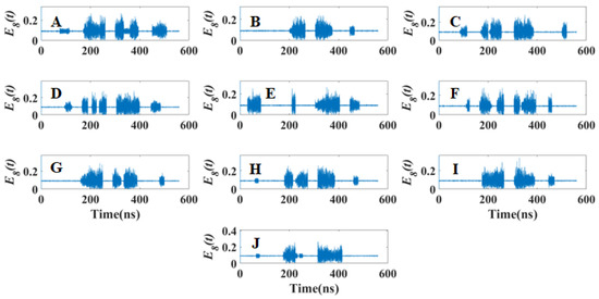
Figure 3.
Temporal trajectories of the output from SL 8 under different fifth samples from digital image sets 0–9 (see Figure 2). (A–J) The temporal trajectories for the fifth samples of digital image sets 0–9, respectively.
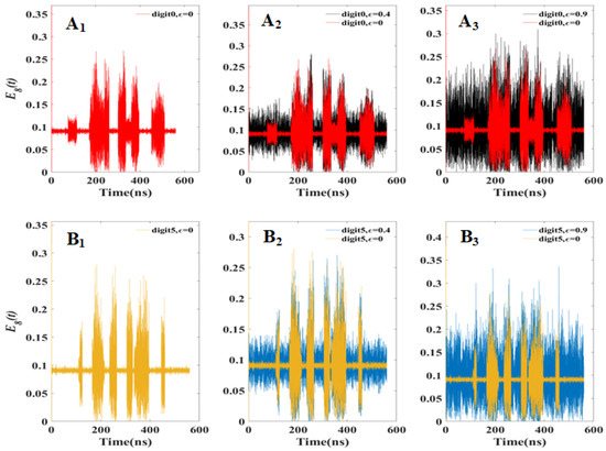
Figure 4.
The temporal trajectories of SL 8 induced by the different fifth samples from digital image sets 0 and 5, which are subjected to different noises. (A) The temporal trajectories of SL 8 induced by the fifth sample from digital image set 0 under = 0; (A) those induced by the fifth sample from digital image set 0 under = 0, 0.4; (A) those induced by the fifth sample from digital image set 0 under = 0, 0.9; (B) those induced by the fifth sample from digital image set 5 under = 0; (B) those induced by the fifth sample from digital image set 5 under = 0, 0.4; (B) those induced by the fifth sample from digital image set 0 under = 0, 0.9.
To further quantify the correlations of the test signal with ten different sets of reference signals, we introduce Spearman correlation coefficients [22] as follows:
where the subscript 8 indicates SL 8. The subscripts d = 0, 1, 2,⋯, 9 show the noise digital image targets 0–9, respectively. The subscripts n = 0, 1, 2,⋯, 9 refer to the sample digit image sets 0–9, respectively. The sample numbers L = 1, 2,⋯, 40. The symbol ⟨ ⟩ represents the time average. is the amplitude of the light from SL 8 output under one noisy digital image d. is the amplitude of light emitted by SL 8 under the Lth sample from the digit image set n. The variable N represents the sample length of or . If = max under a certain noise , one noisy digital image d with noise can be recognized using this condition.
As displayed in Figure 1, suppose that one noisy digital image, as one recognizing target, is injected into ACSCLN 10. The 40 samples from the digital image sets 0–9, as ten sets of reference targets, are injected into the ACSCLNs 0–9, respectively. Under these conditions, we calculate the correlations () of the test signal with ten different sets of reference signals, where the test signal is the output of SL 8 under one noisy digital image d and ten different sets of reference signals are from the output of SL 8 under the 40 samples from the digital image sets 0–9, respectively.The related results are shown in Figure 5. It is found from this figure that if the noise digital images 0–9 are considered as the recognized targets, are the maximums correlation peaks of , , ⋯,, respectively, when ranges from 0 to 0.9. This indicates that the noise digital image targets 0–9 can be recognized well by identifying the maximum correlations.
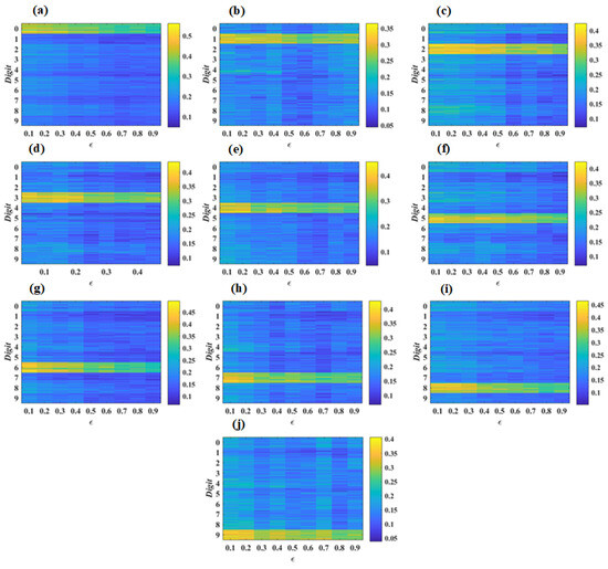
Figure 5.
Evolution maps of the correlations () of the test signal with ten different sets of reference signals, where the test signal is the output of SL 8 under one noisy digital image d and ten different sets of reference signals are from the output of SL 8 under the L samples from the digital image sets 0–9, respectively. Here, = 6.7 ns. (a) via under n = 0, 1, 2,⋯, 9, L = 1, 2, 3, 4,⋯, 40 (the same below); (b) via ; (c) via ; (d) via ; (e) via ; (f) via ; (g) via ; (h) via ; (i) via ; (j) via .
In the following, to verify the recognition accuracy of the noisy digital image targets 0–9, we introduce the expression of the recognition rate () as follows:
where represents the number of correctly recognized samples for each of the noisy digital image targets 0–9. is the total sample number of each of the noisy digital images 0–9 from the digital image sets 0–9, and it is taken as 400. Moreover, the variation of the injection strength in each SL can induce the change of dynamical behavior of SL 8 subjected to the injection of the 40 samples from digital image sets 0–9 in the MNIST dataset or one noisy digital image target. As a result, the correlations () of the test signal with ten sets of reference signals can be varied, and the for each noisy digital image target changes under higher noise. Figure 6 presents the evolution of the recognition rates () for the noisy digital image targets 0–9 in the space of the noise strength under different injection strengths. It is found from Figure 6 that under different injection strengths, the for all noisy digital image targets with higher noise can vary. For example, when = 2.7 ns (see Figure 6A), the RR for each noisy digital image is no less than 88% when is between 0.1 and 0.9. The of all noisy digital images are less than 0.97% when varies from 0.1 to 0.6. While varies from 0.1 to 0.4, the of all noisy digital images except for 0–9 can achieve 100%. If = 0.5, the for the noisy digital images 1–3, 5–7, and 8 can reach 100%. If = 0.6, the for the noisy digital images 3, 7, and 8 can reach 100%. Under = 6.7 ns (see Figure 6B, the RR for each noisy digital image is no less than 86% when is between 0.1 and 0.9. The of all noisy digital images are less than 96% when varies from 0.1 to 0.6. While varies from 0.1 to 0.3, the of all noisy digital images except for 0–9 can achieve 100%. If = 0.4, the for the noisy digital images 1–3, 6, 7, and 9 can reach 100%. If = 0.5, the for the noisy digital images 1, 3, and 7 can reach 100%. Moreover, if = 9.4 (see Figure 6C), the of all noisy digital images are less than 0.85 when changes from 0.1 to 0.9. The of all noisy digital images are less than 94% when varies from 0.1 to 0.6. While varies from 0.1 to 0.3, the of all noisy digital images except for 0–9 can achieve 100%. If = 0.4, the for the noisy digital images 1, 2, 6–8, and 9 can reach 100%. If = 0.5, the for the noisy digital images 7 and 8 can reach 100%. Finally, when = 12.1 ns(see Figure 6D), the of all noisy digital images are less than 81% when varies from 0.1 to 0.9. The of all noisy digital images are less than 93% when varies from 0.1 to 0.6. While varies from 0.1 to 0.2, the of all noisy digital images except for 0–9 can achieve 100%. If = 0.3, the for the noisy digital images 1, 4, 7, and 8 can reach 100%. If = 0.4, the for the noisy digital images 8 can reach 100%. As further observed from this figure, when = 2.7 ns, the for the noisy digital image targets 0–9 exhibit an oscillatory change when is more than 0.6. However, with the further increase of , the oscillatory change of the can occur at lower noise strength.
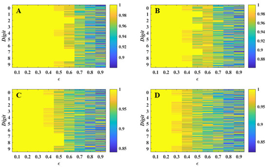
Figure 6.
Evolution maps of the recognition rates () of the noisy digital images 0–9 in the space of the noise strength under different injection strengths (). (A) = 2.7 ns; (B) = 6.7 ns; (C) = 9.4 ns; (D) = 12.1 ns.
To more clearly observe the influence of on the , Figure 7 displays the dependences of the for the noisy digital image target 0 on under different . One sees from Figure 7a that when = 0.2, the of the noisy digital image target 0 is independent of , which varies from 1.5 ns to 15 ns. As shown in Figure 7b, if = 0.4, the exhibits an oscillatory decrease from 1 to 0.97. Under = 0.6, it also shows a decrease in oscillation from 0.965 to 0.93. While = 0.8, it exhibits an oscillatory variation in a small range from 0. 932 to 0.914 when increases from 1.5 ns to 11 ns. But, if further increases from 11 ns to 15 ns, it quickly decreases from 0.914 to 0.84.
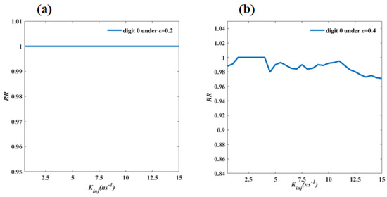
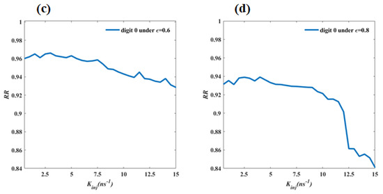
Figure 7.
Dependence of the recognition rates () for the noisy digital image target 0 on the injection strengths () under the different noise strengths (). (a) via under = 0.2; (b) via under = 0.4; (c) via under = 0.6; (d) via under = 0.8.
The results obtained from Figure 5, Figure 6 and Figure 7 show that all noisy digital image targets can be completely recognized under different noises and a certain of injection strength. The recognition accuracies of some noisy digital images can further decrease to a certain extent under higher noise and a fixed injection strength. Under lower noise, the injection strength has little influence on the recognition rate of one noise digital image target. Under higher noise, the recognition rate maintains a higher value (more than 0.9) when the injection strength is no more than 11 ns, but for the larger injection strength, the recognition rate shows further decrease.
4. Conclusions
In conclusion, we utilize the ACSCLN for the recognition of noisy digital image targets 0–9 from different samples of digital image sets 0–9 in the MNIST dataset, where the chaotic lasers network consists of eight asymmetrically coupled semiconductor lasers. In such a chaotic lasers network, one input encodes one noise digital image to be recognized and acts as a driving force. The chaotic signals output from the ACSCLN are encoded in the injected strengths associated with these forces. Here, the outputs from the ACSCLN driven by the 40 samples from digital image sets 0–9 in the MNIST dataset are employed as ten sets of the reference signals; the output of the ACSCLN driven one noisy digital image is utilized as a test signal. Under this condition, one noisy digital image under a certain noise can be recognized by identifying the maximum correlation of its corresponding test signal with ten sets of the reference signals. The studied results show that when the injection strength is fixed at a certain low value, all noisy digital images can be accurately recognized under arbitrary noises. The recognition accuracies of all noisy digital images can further decrease to a certain extent under higher noise and a fixed the injection strength. Under lower noise, the injection strength has little influence on the recognition rate of one noise digital image target. Under higher noise, the recognition rate maintains a higher value (more than 0.9) when the injection strength is no more than a certain value, but for the larger injection strength, the recognition rate exhibits a further decrease. Significantly, our proposed scheme can act as a photonic accelerator to recognize the noisy digital images with noise.
Author Contributions
Conceptualization, D.Z. and W.D.; methodology, D.Z. and W.D.; software, W.D.; formal analysis, W.D., P.H., J.Z., Y.C., Q.W. and T.W.; writing—original draft preparation, W.D.; writing—review and editing, D.Z.; visualization, W.D. All authors have read and agreed to the published version of the manuscript.
Funding
This research was funded by National Natural Science Foundation of China (62075168), Applied Basic Research Foundation of Guangdong Province (2023A1515010726), Major Projects of Guangdong Education Department for Foundation Research and Applied Research (2017KZDX086), an innovation team project of colleges and universities in Guangdong Province (2023KCXTD041, 2021KCXTD051), a special project in key fields of Guangdong Universities: the new generation of communication technology (2020ZDZX3052), and the joint research and development fund of Wuyi University, Hong Kong and Macao (2021WGALH17).
Institutional Review Board Statement
No applicable.
Informed Consent Statement
No applicable.
Data Availability Statement
No applicable.
Conflicts of Interest
The authors declare no conflict of interest.
References
- Kitayama, K.; Notomi, M.; Naruse, M.; Inoue, K.; Kawakami, S.; Uchida, A. Novel frontier of photonics for data processing—Photonic accelerator. APL Photonics 2019, 4, 090901. [Google Scholar] [CrossRef]
- Shastri, B.J.; Tait, A.N.; Ferreira de Lima, T.; Pernice, W.H.; Bhaskaran, H.; Wright, C.D.; Prucnal, P.R. Photonics for artificial intelligence and neuromorphic computing. Nat. Photonics 2021, 15, 102–114. [Google Scholar] [CrossRef]
- Shen, Y.C.; Harris, N.C.; Skirlo, S.; Prabhu, M.; Baehr-Jones, T.; Hochberg, M.; Sun, X.; Zhao, S.; Larochelle, H.; Englund, D. Deep learning with coherent nanophotonic circuits. Nat. Photonics 2017, 11, 441–446. [Google Scholar] [CrossRef]
- Ishihara, T.; Shinya, A.; Inoue, K.; Nozaki, K.; Notomi, M. An integrated nanophotonic parallel adder. ACM J. Emerg. Technol. Comput. Syst. 2018, 14, 1–20. [Google Scholar] [CrossRef]
- Larger, L.; Soriano, M.C.; Brunner, D.; Appeltant, L.; Gutiérrez, J.M.; Pesquera, L.; Mirasso, C.R.; Fischer, I. Photonic information processing beyond Turing: An optoelectronic implementation of reservoir computing. Opt. Express 2012, 20, 3241–3249. [Google Scholar] [CrossRef] [PubMed]
- Takano, K.; Sugano, C.; Inubushi, M.; Yoshimura, K.; Sunada, S.; Kanno, K.; Uchida, A. Compact reservoir computing with a photonic integrated circuit. Opt. Express 2018, 26, 29424–29439. [Google Scholar] [CrossRef] [PubMed]
- Huang, Y.; Zhou, P.; Yang, Y.; Chen, T.; Li, N. Time-delayed reservoir computing based on a two-element phased laser array for image identification. IEEE Photonics J. 2021, 13, 8700109. [Google Scholar] [CrossRef]
- Lee, Y.J.; On, M.B.; Xiao, X.; Proietti, R.; Yoo, S.J.B. Photonic spiking neural networks with event-driven femtojoule optoelectronic neurons based on Izhikevich-inspired model. Opt. Express 2022, 30, 19360–19389. [Google Scholar] [CrossRef] [PubMed]
- Brunner, D.; Soriano, M.C.; Mirasso, C.R.; Fischer, I. Parallel photonic information processing at gigabyte per second data rates using transient states. Nat. Commun. 2013, 4, 1364. [Google Scholar] [CrossRef] [PubMed]
- Zhong, D.Z.; Deng, W.A.; Zhao, K.K.; Hu, Y.L.; Hou, P.; Zhang, J.B. Detections of the position-vectors of the multi targets located in a circular space based on an asymmetric coupling semiconductor lasers network. Opt. Express 2022, 30, 37603–37618. [Google Scholar] [CrossRef] [PubMed]
- Brunner, D.; Fischer, I. Reconfigurable semiconductor laser networks based on diffractive coupling. Opt. Lett. 2015, 40, 3854–3857. [Google Scholar] [CrossRef] [PubMed]
- Ito, H.; Mihana, T.; Horisaki, R.; Naruse, M. Conflict-free joint decision by lag and zero-lag synchronization in laser network. arXiv 2023, arXiv:2307.15373. [Google Scholar]
- Zhong, D.Z.; Yang, H.; Xi, J.T.; Zeng, N.; Xu, Z.; Deng, F.Q. Predictive learning of multi-channel isochronal chaotic synchronization by utilizing parallel optical reservoir computers based on three laterally coupled semiconductor lasers with delay-time feedback. Opt. Express 2021, 29, 5279–5294. [Google Scholar] [CrossRef] [PubMed]
- Zhong, D.Z.; Yang, G.Z.; Xiao, Z.Z.; Ding, Y.; Xi, J.T.; Zeng, N.; Yang, H. Optical chaotic data-selection logic operation with the fast response for picosecond magnitude. Opt. Express 2019, 27, 23357–23367. [Google Scholar] [CrossRef] [PubMed]
- LeCun, Y. The MNIST Database of Handwritten Digits. 1998. Available online: http://yann.lecun.com/exdb/mnist/ (accessed on 19 October 2023).
- Lang, R.; Kobayashi, K. External optical feedback effects on semiconductor injection laser properties. IEEE J. Quantum Electron. 1980, 16, 347–355. [Google Scholar] [CrossRef]
- Xiang, S.Y.; Pan, W.; Li, N.Q.; Zhang, L.Y.; Zhu, H.N. Chaotic unpredictability properties of small network mutually-coupled laser diodes. Opt. Commun. 2013, 311, 294–300. [Google Scholar] [CrossRef]
- Agrawal, G.; Dutta, N. Long Wavelength Semiconductor Lasers, 2nd ed.; Van Nostrand Reinhold: New York, NY, USA, 1993. [Google Scholar]
- Ohtsubo, J. Chaos synchronization and chaotic signal masking in semiconductor lasers with optical feedback. IEEE J. Quantum Electron. 2002, 38, 1141–1154. [Google Scholar] [CrossRef]
- Pisarchik, A.N.; Ruiz-Oliveras, F.R. Optical Chaotic Communication Using Generalized and Complete Synchronization. IEEE J. Quantum Electron. 2010, 46, 279–284. [Google Scholar] [CrossRef]
- Li, N.Q.; Pan, W.; Yan, L.S.; Luo, B.; Zou, X.H.; Xiang, S.Y. Enhanced Two-Channel Optical Chaotic Communication Using Isochronous Synchronization. IEEE J. Sel. Top. Quantum Electron. 2013, 19, 0600109. [Google Scholar]
- Kim, S.; Ouyang, M.; Zhang, X. Compute spearman correlation coefficient with Matlab/CUDA. In Proceedings of the 2012 IEEE International Symposium on Signal Processing and Information Technology (ISSPIT), Ho Chi Minh City, Vietnam, 12–15 December 2012; pp. 000055–000060. [Google Scholar]
Disclaimer/Publisher’s Note: The statements, opinions and data contained in all publications are solely those of the individual author(s) and contributor(s) and not of MDPI and/or the editor(s). MDPI and/or the editor(s) disclaim responsibility for any injury to people or property resulting from any ideas, methods, instructions or products referred to in the content. |
© 2023 by the authors. Licensee MDPI, Basel, Switzerland. This article is an open access article distributed under the terms and conditions of the Creative Commons Attribution (CC BY) license (https://creativecommons.org/licenses/by/4.0/).