Quantifying Seasonal Shoreline Distribution of Water Hyacinth (Eichhornia crassipes) in Winam Gulf, Lake Victoria

Abstract

Water hyacinth (Eichhornia crassipes) is among the world’s most invasive aquatic macrophytes, yet quantitative models of shoreline preference remain absent for Lake Victoria. This study developed a distance-based quantitative framework for spatial distribution and decay modelling to quantify seasonal nearshore accumulation dynamics in Winam Gulf, Kenya, using Sentinel-2 imagery. A Support Vector Machine classifier with polygon-mean feature extraction achieved 94–96% accuracy, supported by strong spectral separability (Jeffries–Matusita distance > 1.9 in six bands). During peak dry season, water hyacinth covered 405.81 km² (27.1% of gulf area) and occurred significantly closer to shore than open water (mean preference = 687.9 m; 95% CI: 616.6–753.7 m; p < 0.001). Water hyacinth was 3.10 times more likely than open water to occur within 100 m of shoreline, with 48% of biomass concentrated within 2 km. A power-law decay model of odds ratio with shoreline distance provided superior fit (R² = 0.870, F = 10.06, p = 0.047) compared to exponential decay (R² = 0.477, p = 0.378). Critically, pronounced nearshore preference occurred only during dry-season conditions (+687.9 m to +1946.6 m), while wet–dry transition periods showed no significant preference (−124.2 m; p = 1.00), supporting wind-driven Stokes drift as the dominant transport mechanism and enabling seasonal prioritization of nearshore management interventions.

1. Introduction

Water hyacinth (Eichhornia crassipes) ranks among the world’s most problematic invasive aquatic plants, causing severe ecological and socioeconomic impacts across tropical and subtropical freshwater systems [1,2,3]. Native to the Amazon basin of South America, this free-floating macrophyte has colonized freshwater bodies across six continents, facilitated by its ornamental trade value, rapid vegetative reproduction, and broad environmental tolerance [3,4]. Under favourable nutrient conditions, water hyacinth populations exhibit exponential growth rates, with biomass doubling times of 6–18 days, enabling rapid transformation of open water into dense vegetative mats [5,6]. Water hyacinth invasion causes severe ecological impacts, including reduced light penetration, hypoxic conditions, and disrupted aquatic food webs [7,8], with socioeconomic costs in Africa alone exceeding USD 20–50 million annually through navigation obstruction, infrastructure interference, and reduced fisheries productivity [9,10].

Lake Victoria, the world’s second-largest freshwater lake by surface area (68,800 km²) and largest tropical lake, has experienced recurrent water hyacinth infestations since the species was first documented in 1989 [11,12]. The lake supports over 40 million people across Kenya, Uganda, and Tanzania through artisanal fisheries, transportation, and domestic water supply [12,13]. Water hyacinth proliferation in Lake Victoria has been linked to progressive eutrophication driven by nutrient loading from agricultural runoff, urban wastewater discharge, and atmospheric deposition [14,15], creating conditions that favour explosive macrophyte growth. Winam Gulf, a shallow semi-enclosed embayment in northeastern Lake Victoria, has been identified as one of the most severely affected areas, with historical coverage exceeding 35% of gulf surface area during the 1997–1998 outbreak peak [16]. Despite decades of mechanical harvesting and biological control efforts, water hyacinth remains a persistent management challenge [17,18].

Remote sensing has emerged as an essential tool for monitoring aquatic invasive species across large spatial extents with high temporal frequency [19,20,21]. Satellite-based multispectral sensors can detect floating vegetation through characteristic spectral signatures, particularly the pronounced increase in near-infrared (NIR) reflectance caused by internal leaf scattering, contrasted with strong NIR absorption by water [22,23]. This spectral contrast enables discrimination of floating macrophytes from open water using vegetation indices such as the Normalized Difference Vegetation Index [24], Normalized Difference Water Index [25], and Floating Algae Index [26]. Numerous studies have applied remote sensing to map water hyacinth in African lakes [27,28,29,30,31,32,33,34,35]. Fusilli et al. [36] used MODIS imagery to track water hyacinth dynamics in Lake Victoria from 2000 to 2010, documenting seasonal expansion-contraction cycles. Dube et al. [27] achieved classification accuracies exceeding 90% for water hyacinth in South African impoundments using Landsat 8 and machine learning algorithms, while Thamaga and Dube [28] demonstrated the value of Sentinel-2 red edge bands for discriminating water hyacinth from other aquatic vegetation.

Among available satellite platforms, Sentinel-2 is particularly well-suited for monitoring dynamic aquatic macrophyte populations owing to its 10 m spatial resolution, red-edge spectral bands, and 5-day revisit capability [37,38,39,40]. Machine learning classifiers, especially Support Vector Machines, have shown superior performance for aquatic vegetation mapping in optically complex inland waters [27,28], and polygon-mean feature extraction approaches have been shown to reduce spectral noise relative to pixel-based methods [21,41].

While extensive research has focused on mapping water hyacinth extent and temporal dynamics, quantitative understanding of spatial distribution patterns within affected water bodies remains limited [9,18]. Most studies treat water hyacinth distribution as spatially homogeneous within mapped extents [27,36], yet field observations consistently indicate heterogeneous distributions with concentrations in sheltered bays, along lee shorelines, and near nutrient sources [9,16]. The relationship between floating vegetation distribution and shoreline proximity has been qualitatively documented but not rigorously quantified. Kateregga and Sterner [9] noted that water hyacinth in Lake Victoria “tends to accumulate along shorelines and in protected bays,” attributing this pattern to wind-driven transport and reduced wave exposure. Albright et al. [16] observed that persistent infestations in Winam Gulf occurred “within 2–3 km of shore.” However, these observations lack quantitative precision needed to inform spatial management strategies.

Wind-driven wave action is a primary mechanism governing the spatial distribution of floating vegetation in large water bodies [42,43]. Surface waves generate net mass transport in the direction of wave propagation through Stokes drift, which can substantially affect floating objects [44,45]. In fetch-limited shallow water environments, wave energy decays exponentially with distance from shore due to bottom friction and geometric spreading [46,47]. This process creates distinct hydrodynamic zones: high-energy offshore areas where vegetation disperses, transition zones where accumulation begins, and low-energy nearshore zones where stable mat formation occurs [42,48]. If floating vegetation distribution is governed primarily by wave-driven transport, occurrence probability should decline exponentially with shoreline distance, following wave energy attenuation patterns [43,46]. However, alternative functional forms such as power law relationships may emerge if bathymetric gradients are non-linear or if secondary accumulation zones exist at intermediate distances [49,50]. Testing these alternative models empirically requires spatially explicit quantitative analysis.

Despite extensive water hyacinth mapping research, quantitative models of shoreline preference remain absent for Lake Victoria. Understanding spatial distribution patterns has practical significance: mechanical harvesting operations are typically limited to within 2–5 km of shore-based facilities due to operational constraints [18], yet the proportion of biomass within accessible zones remains unquantified. Furthermore, seasonal variability in wind patterns may modulate shoreline preference, but temporal dynamics of spatial distribution have not been systematically analysed [51,52]. This study aims to address these knowledge gaps by quantifying the spatial relationship between water hyacinth distribution and shoreline proximity in Winam Gulf, Lake Victoria. The specific objectives are: (1) to clarify the spatial distribution pattern of water hyacinth and quantify its seasonal variability using Sentinel-2 multispectral imagery; (2) to establish and compare quantitative models of the decay in shoreline preference with distance, tested against multiple functional forms; and (3) to translate spatial findings into evidence-based recommendations for prioritising mechanical harvesting zones.

This study provides the first quantitative estimate of shoreline preference magnitude for water hyacinth in Lake Victoria, develops theoretically motivated spatial decay models testable across sites and time periods, demonstrates a rigorous methodological framework integrating high-resolution satellite imagery with machine learning classification and multi-model spatial analysis, and translates findings into actionable management guidance based on quantitative evidence. The approach is transferable to other aquatic invasive species and water bodies globally.

2. Materials and Methods

2.1. Study Area

Winam Gulf (also known as Nyanza Gulf or Kavirondo Gulf) is a shallow, semi-enclosed embayment located in the northeastern corner of Lake Victoria, Kenya (approximately 0°06′ S to 0°32′ S, 34°13′ E to 34°52′ E). The gulf extends approximately 74 km in length and 50 km in width, with a total surface area of approximately 1493 km² and a mean depth of 4–6 m [51]. The gulf connects to the main body of Lake Victoria through a narrow opening (~3 km wide) near Rusinga Island, which restricts water exchange and creates a semi-enclosed system conducive to water hyacinth accumulation.

Winam Gulf receives substantial nutrient inputs from the Nyando, Sondu-Miriu, and Kibos rivers, as well as urban and agricultural runoff from Kisumu City and surrounding catchments. These nutrient loadings, combined with the gulf’s sheltered morphology, shallow bathymetry, and warm tropical climate (mean annual temperature: 23–25 °C), create optimal conditions for water hyacinth proliferation. The gulf has experienced recurrent water hyacinth outbreaks since the 1990s, making it one of the most severely affected areas in Lake Victoria [16,36].

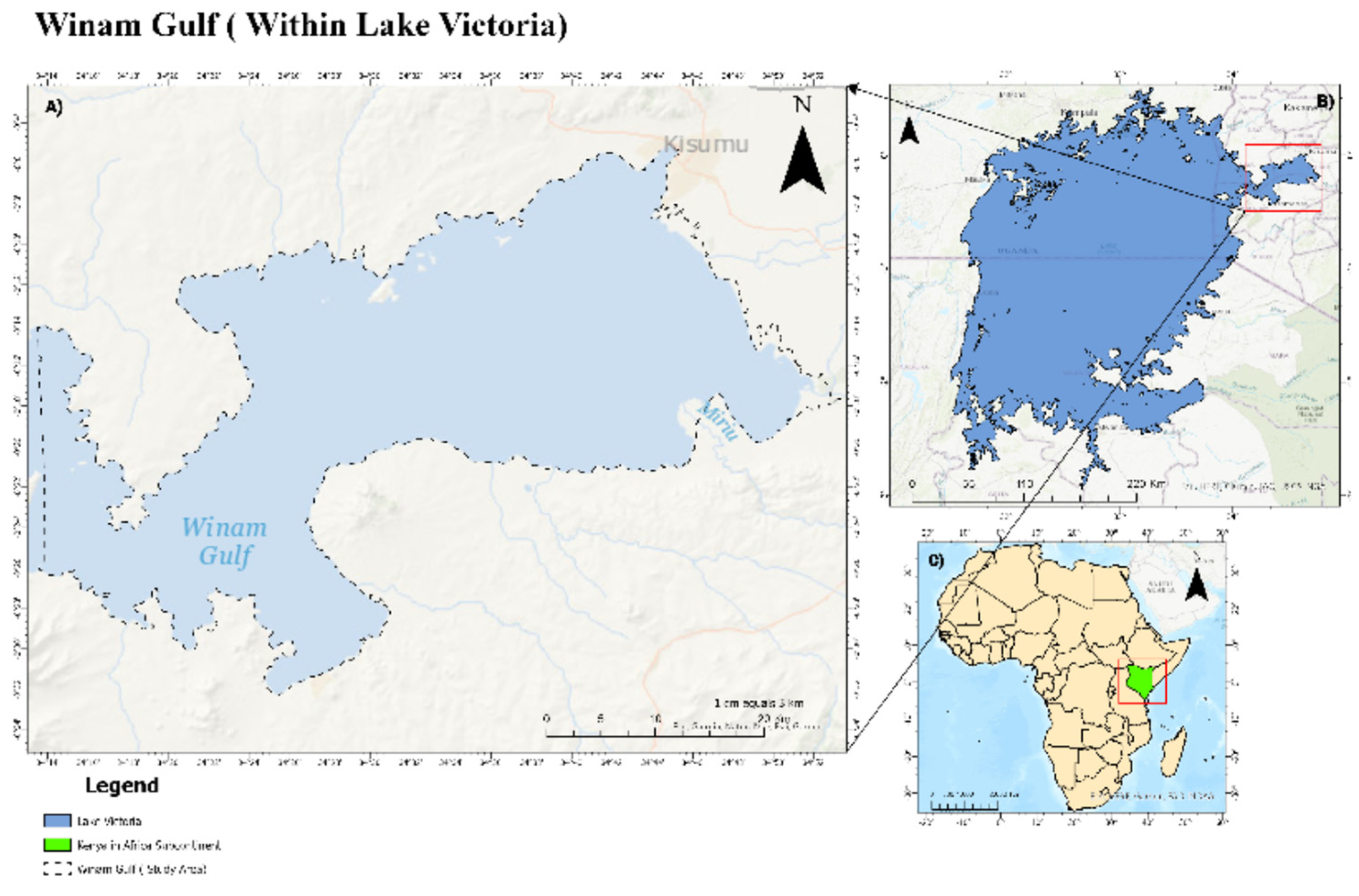
The gulf experiences distinct seasonal hydrodynamic regimes. During the dry season (June–October), persistent southeasterly trade winds generate surface waves that propagate toward the northern and western shorelines, potentially driving shoreward transport of floating vegetation. During the wet season (March–May), variable wind directions, elevated rainfall, higher lake levels, and increased riverine discharge create more complex circulation patterns. This seasonal contrast motivated the multi-temporal design of this study (Figure 1).

2.2. Satellite Data Acquisition and Image Selection

Three cloud-free Sentinel-2 images were selected in advance to capture contrasting seasonal hydrodynamic conditions in Winam Gulf. The first image, from 31 May 2020, represents the wet-dry seasonal transition, a period marked by variable wind directions, elevated rainfall, and increased riverine discharge. The second, from 8 October 2020, corresponds to the early dry season, reflecting the onset of persistent southeasterly trade winds. The third, from 23 October 2020, represents the peak dry season, when southeasterly wind forcing is sustained and dominant.

Date selection was based on: (1) cloud cover <5% over the study area, (2) representation of distinct seasonal hydrodynamic regimes documented in prior Lake Victoria studies [51], and (3) availability of high-quality Level-2A atmospherically corrected imagery [53]. The October dates were specifically chosen to capture potential temporal variation within the dry season, as previous studies have documented intra-seasonal variability in water hyacinth distribution [16].

2.3. Training Data Collection

Training polygons for supervised classification were manually digitised through visual interpretation of the Sentinel-2 imagery using a false-colour composite (NIR-Red-Green) to enhance vegetation detection. Two classes were defined: water hyacinth (H) and open water (W). Polygons were delineated based on spectral characteristics, with water hyacinth appearing as bright magenta-red patches due to high NIR reflectance from chlorophyll-rich floating vegetation, and open water appearing dark due to strong absorption in NIR wavelengths. For the peak dry season image, a total of 246 training polygons were digitised, comprising 174 water hyacinth polygons (70.7%) and 72 open water polygons (29.3%). Training samples were distributed across the entire gulf to capture spectral variability associated with different water hyacinth mat densities, water depths, and turbidity conditions. Polygon sizes ranged from approximately 500 m² to 50,000 m², ensuring representation of both small, fragmented patches and large contiguous mats.

2.4. Spectral Characterisation and Separability Analysis

Prior to classification, spectral separability between water hyacinth and open water was quantified to assess the feasibility of accurate discrimination and to inform classification approach selection. Mean reflectance values were extracted for each training polygon across all ten spectral bands, yielding a representative spectral signature for each training sample.

Spectral separability was quantified using the Jeffries–Matusita (JM) distance [54], a widely used metric in remote sensing that ranges from 0 (complete spectral overlap) to 2 (complete separation). For each band, the JM distance was calculated as follows:

$$JM=2(1-exp(-B\left)\right)$$

(1)

where B is the Bhattacharyya distance:

$$B={\displaystyle \frac{1}{8}}({\mu }_1-{\mu }_2{)}^2/{\sigma }^2+{\displaystyle \frac{1}{2}}ln\left({\displaystyle \frac{{\sigma }^2}{{\sigma }_1{\sigma }_2}}\right)$$

(2)

where μ₁ and μ₂ are the class means, σ₁ and σ₂ are the class standard deviations, and σ² = (σ₁² + σ₂²)/2 is the pooled variance. Following Richards and Jia [55], JM values exceeding 1.9 indicate excellent separability, values between 1.7 and 1.9 suggest good separability, and values below 1.0 indicate poor separability.

To provide independent validation of the SVM classification, three established vegetation indices were calculated for the classified image: (1) Normalized Difference Vegetation Index (NDVI = (NIR − Red)/(NIR + Red) [24]), (2) Normalized Difference Water Index (NDWI = (Green − NIR)/(Green + NIR) [25]), and (3) Floating Algae Index (FAI = NIR − (Red + (SWIR1 − Red) × (λ_NIR − λ_Red)/(λ_SWIR1 − λ_Red)) [26]). In the FAI formula, λ_NIR, λ_Red, and λ_SWIR1 denote the central wavelengths of the NIR (B8, 842 nm), Red (B4, 665 nm), and SWIR1 (B11, 1610 nm) bands, respectively. Mean values of each index were compared between SVM-classified water hyacinth and open water pixels to confirm alignment with expected patterns documented in the literature.

2.5. Image Classification

A Support Vector Machine (SVM) classifier with a radial basis function (RBF) kernel was employed for supervised classification. SVM was selected for its demonstrated effectiveness in classifying aquatic vegetation in optically complex inland waters [27,56,57,58] and its robustness to high-dimensional feature spaces; although forest classifiers have also shown strong performance in remote sensing applications [59]. To mitigate overfitting and reduce noise inherent in pixel-level classification, a polygon-mean approach was adopted [41,60]. For each training polygon, the mean spectral signature was calculated by averaging reflectance values across all pixels within the polygon for each of the ten spectral bands.

Prior to model training, features were standardised using z-score normalisation (mean = 0, standard deviation = 1) to ensure equal contribution of all spectral bands to the classification decision. The classification decision was therefore made at the polygon level (using mean spectral signatures), not on individual pixels; the resulting polygon-level labels were then projected spatially to produce the final binary raster. The SVM classifier was configured with the following parameters: C = 1.0 (regularisation parameter), gamma = ‘scale’ (kernel coefficient set to 1/(n_features × variance)), and balanced class weights (class_weight = ‘balanced’) to explicitly counteract the training polygon imbalance between hyacinth (n = 174) and water (n = 72) classes; this weighting increases the penalty for misclassifying minority-class samples, preventing the classifier from simply predicting the majority class.

The training dataset was partitioned using stratified random sampling, with 70% (n = 172 polygons) allocated for model training and 30% (n = 74 polygons) reserved for independent accuracy assessment. Model performance was further evaluated using 5-fold cross-validation on the training subset to assess generalisation ability and detect potential overfitting. Classification accuracy was assessed [61,62] using the following metrics: (1) overall accuracy (OA), defined as the proportion of correctly classified test samples; (2) Cohen’s kappa coefficient (κ), which accounts for chance agreement; (3) precision (user’s accuracy for water hyacinth); (4) recall (producer’s accuracy for water hyacinth); and (5) F1-score, the harmonic mean of precision and recall. A confusion matrix was generated to quantify commission and omission errors for each class.

Following validation, the trained SVM model was applied to the entire Sentinel-2 image to generate a binary classification map. Classification was performed using a moving window approach with 1000 × 1000-pixel tiles to manage computational memory requirements.

2.6. Shoreline Distance Calculation

Shoreline distance was calculated as the Euclidean distance from each pixel centroid to the nearest point on the Winam Gulf shoreline boundary. The shoreline boundary was extracted from a digitised vector polygon of the study area in the projected coordinate system UTM Zone 36S [63] to ensure distance measurements in metres.

For each pixel location within the classified water area, the minimum distance to the shoreline was computed using the following procedure: (1) pixel centroids were derived from the raster coordinate system using affine transformation parameters; (2) shoreline vertices were extracted from the boundary polygon (40,933 coordinate points); and (3) the minimum Euclidean distance between each pixel centroid and all shoreline vertices was calculated using the cdist function from the SciPy spatial distance module [64]. This process generated a continuous distance-to-shore raster with values ranging from 0 m (at shoreline) to a maximum of approximately 24,200 m at the gulf centre.

2.7. Shoreline Preference Analysis

2.7.1. Descriptive Statistics

Distance-to-shore values were extracted separately for pixels classified as water hyacinth and open water. Descriptive statistics [65] including mean, median, standard deviation, 25th percentile (Q1), and 75th percentile (Q3) were calculated for each class to characterise their respective distance distributions.

Shoreline preference strength was quantified as the difference between the mean distance of open water pixels and the mean distance of water hyacinth pixels:

$$Preference Strength \left(m\right)={\mu }_{water}-{\mu }_{hyacinth}$$

(3)

where μ_water and μ_hyacinth are the mean distances for open water and water hyacinth, respectively. Positive values indicate that water hyacinth occurs closer to the shoreline than would be expected under a spatially random distribution.

2.7.2. Bootstrap Confidence Intervals

To quantify uncertainty in the preference strength estimate, 95% confidence intervals were calculated using a bootstrap resampling procedure [66]. A total of 1000 bootstrap iterations were performed, with each iteration randomly sampling (with replacement) 10,000 pixels from each class to ensure computational feasibility while maintaining statistical representativeness. The preference strength was recalculated for each bootstrap sample, and the 2.5th and 97.5th percentiles of the resulting distribution defined the 95% confidence interval bounds.

2.7.3. Shoreline Buffer Zone Analysis

Five concentric buffer zones were delineated from the shoreline at distances of 100 m, 250 m, 500 m, 1000 m, and 2000 m to examine the spatial distribution of water hyacinth relative to shoreline proximity. These distances were selected to capture near-shore accumulation patterns (100–500 m), intermediate zones (1000 m), and the transition to open water (2000 m).

For each buffer zone, the following metrics were calculated:

Proportion within buffer: The percentage of total water hyacinth pixels occurring within each buffer distance from shore.

Odds ratio (OR): The odds of water hyacinth presence within the buffer relative to outside the buffer, compared to the equivalent odds for open water:

$$OR={\displaystyle \frac{H_{in}/H_{out}}{W_{in}/W_{out}}}$$

(4)

where H_in and H_out represent water hyacinth pixel counts inside and outside the buffer, respectively, and W_in and W_out represent open water pixel counts. OR > 1 indicates preferential association with the near-shore zone.

95% confidence intervals for odds ratios: Calculated using the standard error of the log odds ratio under the assumption of independent observations:

$$SE\left(lnOR\right)=\sqrt{{\displaystyle \frac{1}{H_{in}}}+{\displaystyle \frac{1}{H_{out}}}+{\displaystyle \frac{1}{W_{in}}}+{\displaystyle \frac{1}{W_{out}}}}$$

(5)

$$95\% CI=exp(lnOR\pm 1.96\times SE)$$

(6)

2.7.4. Statistical Testing with Multiple Comparisons Correction

The Mann–Whitney U test [67] was employed to assess whether the distance distributions of water hyacinth and open water pixels differed significantly. This non-parametric test [68] was selected because distance data exhibited right-skewed distributions inconsistent with normality assumptions. Chi-square tests of independence (χ²) [69] were conducted for each buffer zone to test the null hypothesis that water hyacinth and open water were distributed independently of shoreline proximity. To account for multiple hypothesis testing across five buffer zones, the Bonferroni correction [70] was applied, adjusting the significance threshold from α = 0.05 to α = 0.01 (0.05/5 tests).

Effect size was quantified using Cohen’s d, calculated as the standardised mean difference:

$$d={\displaystyle \frac{{\mu }_{water}-{\mu }_{hyacinth}}{{\sigma }_{pooled}}}$$

(7)

where σ_pooled = √((σ²_water + σ²_hyacinth)/2) is the pooled standard deviation.

2.7.5. Spatial Decay Modelling

To characterise the relationship between odds ratio and buffer distance, four candidate models were fitted and compared:

Exponential decay: OR(d) = a × exp(−b × d)

(8)

Power law: OR(d) = a × (d + 1)^b

(9)

Logarithmic: OR(d) = a + b × ln(d + 1)

(10)

Linear: OR(d) = a + b × d

(11)

where OR(d) is the odds ratio at distance d (metres), and a and b are model parameters. The offset of +1 in the power law and logarithmic models prevents undefined values at d = 0. Model parameters were estimated using non-linear least squares regression via the Levenberg–Marquardt algorithm [71] implemented in SciPy’s curve_fit function [64]. Goodness-of-fit was assessed using the coefficient of determination (R²):

$$R^2=1-{\displaystyle \frac{S{S}_{res}}{S{S}_{tot}}}$$

(12)

Model selection was based on Akaike Information Criterion [72,73]:

$$AIC=n\times ln(S{S}_{res}/n)+2k$$

(13)

where n is the number of observations (buffer zones), and k is the number of model parameters. Lower AIC values indicate better model fit relative to complexity. For the exponential model, the half-distance (d_1/2), defined as the distance at which the odds ratio declines to half of its initial value, was calculated as follows:

$$d_{1/2}={\displaystyle \frac{ln\left(2\right)}{b}}$$

(14)

2.8. Temporal Validation

To assess the temporal robustness of observed spatial patterns, the complete classification and shoreline preference analysis pipeline was applied independently to two additional Sentinel-2 images: 31 May 2020 (wet-dry transition) and 8 October 2020 (early dry season). Each date was processed with its own independently digitised training polygons to avoid cross-date contamination.

Consistency was evaluated by comparing preference strength, odds ratios, model parameters, and statistical significance across dates. The coefficient of variation (CV) was calculated to quantify temporal variability in preference strength:

$$CV={\displaystyle \frac{\sigma }{\mu }}\times 100\%$$

(15)

where σ is the standard deviation and μ is the mean of preference strength across dates.

2.9. Software and Reproducibility

All analyses were conducted using Python 3.9 [74] with the following libraries: Rasterio 1.3 [75] for raster input/output and spatial operations, GeoPandas 0.12 [76] for vector processing and coordinate transformations, Scikit-learn 1.2 [77] for machine learning classification and cross-validation, SciPy 1.10 [64] for statistical tests and non-linear optimisation, NumPy 1.24 [78] for numerical array operations, Matplotlib 3.6 [79] and Seaborn 0.12 [80] for data visualisation.

3. Results

3.1. Spectral Characteristics and Separability

3.1.1. Spectral Signatures

Analysis of mean spectral signatures extracted from 246 training polygons revealed distinct reflectance patterns between water hyacinth and open water across the electromagnetic spectrum. Water hyacinth exhibited characteristic vegetation spectral properties, with relatively low reflectance in the visible region due to chlorophyll absorption (Blue: 1156.4 ± 441.2; Green: 1406.4 ± 312.8; Red: 1321.8 ± 292.1) and a pronounced increase in reflectance in the red edge and NIR regions (Red Edge 3: 4408.6 ± 1548.3; NIR: 4322.7 ± 1503.2). This NIR plateau is characteristic of healthy photosynthetically active vegetation and reflects strong scattering from internal leaf mesophyll structures (

Table 1. Mean spectral signatures and separability metrics for water hyacinth (n = 174 polygons) and open water (n = 72 polygons).

Band	Wavelength (nm)	Hyacinth Mean ± SD	Water Mean ± SD	Difference	JM Distance	Separability
B2 (Blue)	490	1156.4 ± 441.2	1597.8 ± 312.5	−441.4	1.967	Excellent
B3 (Green)	560	1406.4 ± 312.8	1656.3 ± 389.7	−249.9	0.998	Moderate
B4 (Red)	665	1321.8 ± 292.1	1912.9 ± 367.2	−591.1	1.999	Excellent
B5 (Red Edge 1)	705	2155.9 ± 509.6	1585.9 ± 401.3	+570.0	1.124	Moderate
B6 (Red Edge 2)	740	4408.6 ± 1548.3	1586.0 ± 401.2	+2822.6	1.935	Good
B7 (Red Edge 3)	783	4676.1 ± 1603.9	1589.3 ± 401.5	+3086.8	1.942	Good
B8 (NIR)	842	4322.7 ± 1503.2	1321.9 ± 375.8	+3000.8	1.937	Good
B8A (Narrow NIR)	865	4447.0 ± 1559.3	1341.9 ± 379.4	+3105.1	1.924	Good
B11 (SWIR1)	1610	1812.1 ± 440.3	1273.0 ± 348.1	+539.1	1.226	Moderate
B12 (SWIR2)	2190	1349.0 ± 295.7	1183.3 ± 332.4	+165.7	0.756	Poor

JM = Jeffries–Matusita distance. Separability interpretation: >1.9 = Excellent, 1.7–1.9 = Good, 1.0–1.7 = Moderate, <1.0 = Poor [55].

).

3.1.2. Spectral Separability

Jeffries–Matusita (JM) distance analysis confirmed excellent spectral separability between water hyacinth and open water in six of ten Sentinel-2 bands. The red (B4) band exhibited the highest separability (JM = 1.999), followed closely by blue (B2; JM = 1.967), red edge 3 (B7; JM = 1.942), NIR (B8; JM = 1.937), red edge 2 (B6; JM = 1.935), and narrow NIR (B8A; JM = 1.924). These JM values exceed the 1.9 threshold indicative of excellent separability [55].

3.1.3. Validation Against Established Indices

Classification results were validated against three established vegetation indices (

Table 2. Validation of SVM classification against established vegetation indices.

Index	Hyacinth Mean ± SD	Water Mean ± SD	Difference	Expected Pattern	Agreement
NDVI	0.261 ± 0.321	−0.318 ± 0.137	+0.580	H > W	✓
NDWI	−0.075 ± 0.325	0.415 ± 0.112	−0.490	H < W	✓
FAI	831.6 ± 1076.7	−270.7 ± 159.2	+1102.4	H >> W	✓

H = Water hyacinth; W = Open water; ✓ = agreement between the classified spectral difference and the expected spectral pattern direction (H > W or H < W).

). Water hyacinth pixels exhibited significantly higher NDVI values (mean = 0.261 ± 0.321) compared to open water (mean = −0.318 ± 0.137; Welch t = 3516, df = 4.6 × 10⁶, p < 0.001; Cohen’s d = 2.35). The NDVI mean of 0.261 is consistent with published values for floating water hyacinth mats (typically 0.2–0.5), which are lower than dense terrestrial canopies due to submerged stems, partial canopy closure, and mixed pixels at mat edges [81]; the high SD (0.321) reflects genuine within-class variability across mat densities and growth stages rather than a methodological error. NDWI values showed the inverse pattern, with water hyacinth exhibiting lower values (mean = −0.075 ± 0.325) than open water (mean = 0.415 ± 0.112; Cohen’s d = −2.02, p < 0.001). The Floating Algae Index (FAI) showed the strongest discrimination, with water hyacinth pixels exhibiting FAI values of 831.6 ± 1076.7 compared to −270.7 ± 159.2 for open water (Cohen’s d = 1.43, p < 0.001). While 2-SD ranges overlap for all three indices when considered individually, this is expected given within-class variability; the SVM classifier uses all ten bands simultaneously, and the combination of large effect sizes (Cohen’s d = 1.4–2.3) and pixel-level discrimination probabilities of 84–95% confirms robust class separation.

3.2. Classification Accuracy

The SVM classifier demonstrated consistently high performance across all three analysis dates (

Table 3. Classification accuracy metrics across all analysis dates.

Season	Training Polygons	OA	κ	Precision	Recall	F1	CV Accuracy
Peak Dry	246 (174 H, 72 W)	0.96	0.90	0.95	0.96	0.95	0.96 ± 0.02
Wet-Dry Transition	363 (235 H, 128 W)	0.94	0.88	0.93	0.94	0.93	0.94 ± 0.02
Early Dry	369 (217 H, 152 W)	0.95	0.89	0.94	0.95	0.94	0.95 ± 0.01

OA = Overall Accuracy; κ = Cohen’s kappa; CV = Cross-validation; H = Hyacinth; W = Water.

). Overall accuracy ranged from 0.94 to 0.96, indicating robust discrimination between water hyacinth and open water across contrasting seasonal conditions. Cohen’s kappa values (0.88–0.90) reflected strong agreement between classified outputs and reference data beyond chance.

Classification performance was highest during peak dry-season conditions, when spectral separability between classes was greatest. Precision, recall, and F1-scores ranged from 0.93 to 0.96 for both classes across all seasons, with slightly reduced performance during the wet–dry transition period, likely reflecting increased spectral mixing and turbidity effects. Five-fold cross-validation results showed low variability (standard deviation ≤ 0.02), indicating stable model generalisation and minimal sensitivity to training sample selection. Confusion matrix analysis for the peak dry season (

Table 4. Confusion matrix for the peak dry season data.

	Predicted Water	Predicted Hyacinth	Total	User’s Accuracy
Actual Water	21	1	22	0.955
Actual Hyacinth	2	50	52	0.962
Total	23	51	74	—
Producer’s Accuracy	0.913	0.980	—	OA = 0.959, κ = 0.90

) showed limited misclassification between classes, with most errors associated with boundary pixels in transitional nearshore zones. Overall, classification accuracy was sufficient to support subsequent spatial and distance-based modelling analyses.

3.3. Water Hyacinth Extent and Distribution

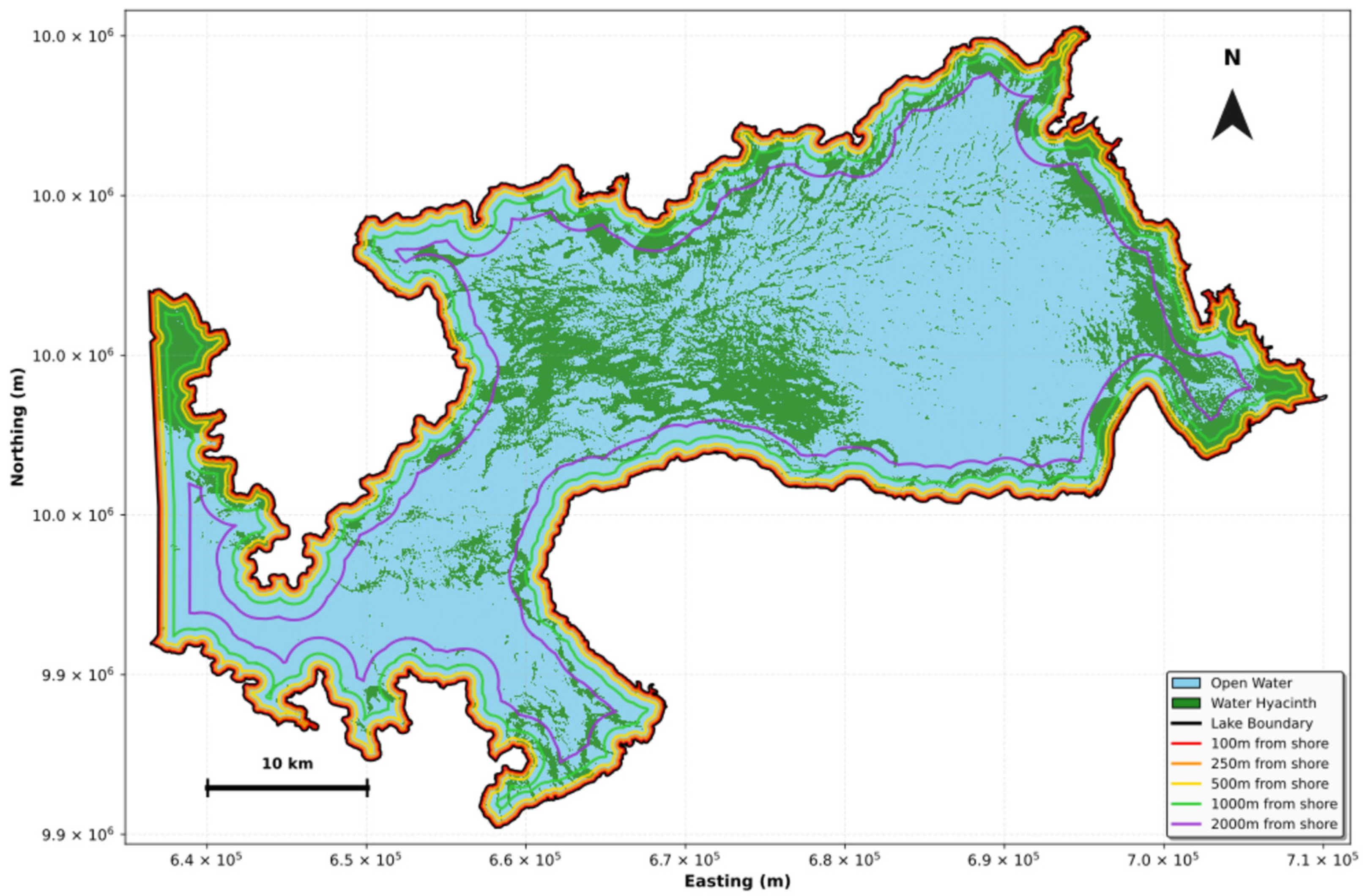
Application of the trained SVM classifier to the peak dry season image identified 4,058,134 pixels as water hyacinth, representing 27.1% of the classified water surface area (

Table 5. Water hyacinth extent across analysis dates.

Season	Hyacinth Pixels	Water Pixels	Hyacinth (%)	Area (km2)
Peak Dry	4,058,134	10,895,239	27.1	405.81
Wet-Dry Transition	3,576,783	11,376,590	23.9	357.68
Early Dry	3,125,116	11,828,257	20.9	312.51

). Water hyacinth coverage totalled 405.81 km², while open water comprised 10,895,239 pixels (1089.52 km²), representing 72.9% of the water surface (Figure 2).

3.4. Shoreline Preference During Dry Season Peak

3.4.1. Distance Distribution Characteristics

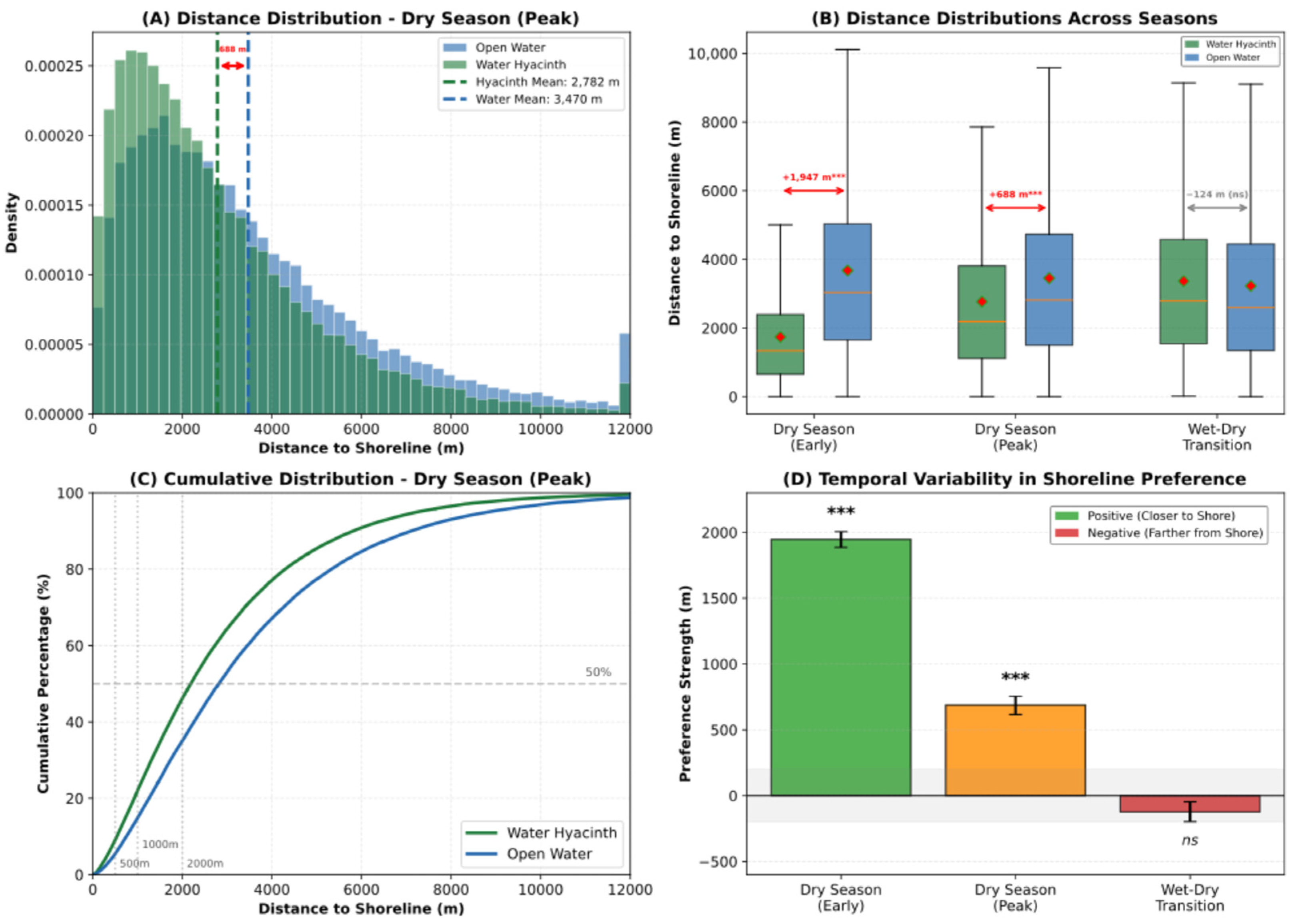
Analysis of distance-to-shore distributions revealed a pronounced spatial preference for near-shore habitats among water hyacinth pixels (

Table 6. Descriptive statistics for distance-to-shore distributions during peak dry season.

Class	n (Pixels)	Mean (m)	SD (m)	Median (m)	Min (m)	Max (m)
Water Hyacinth	4,058,134	2781.9	2292.2	2119.4	0.0	11,750.8
Open Water	10,895,239	3469.8	2720.5	2799.4	0.0	11,901.4
Difference	—	687.9	—	680.0	—	—

). Water hyacinth occurred at a mean distance of 2781.9 m from the shoreline (SD = 2292.2 m; median = 2119.4 m), compared to a mean distance of 3469.8 m for open water pixels (SD = 2720.5 m; median = 2799.4 m). The difference of 687.9 m represents a consistent shoreward displacement of water hyacinth relative to the overall water surface. Bootstrap resampling (1000 iterations) established a 95% confidence interval of 616.6 m to 753.7 m for the preference strength, confirming the robustness of this estimate. The Mann–Whitney U test confirmed that water hyacinth distances were significantly lower than open water distances (U = 4.31 × 10⁹, p < 0.001, one-tailed).

The effect size, quantified using Cohen’s d, was 0.273. In operational terms, the 687.9 m displacement represents 34.4% of typical mechanical harvester reach (~2000 m) (Figure 3).

3.4.2. Buffer Zone Analysis

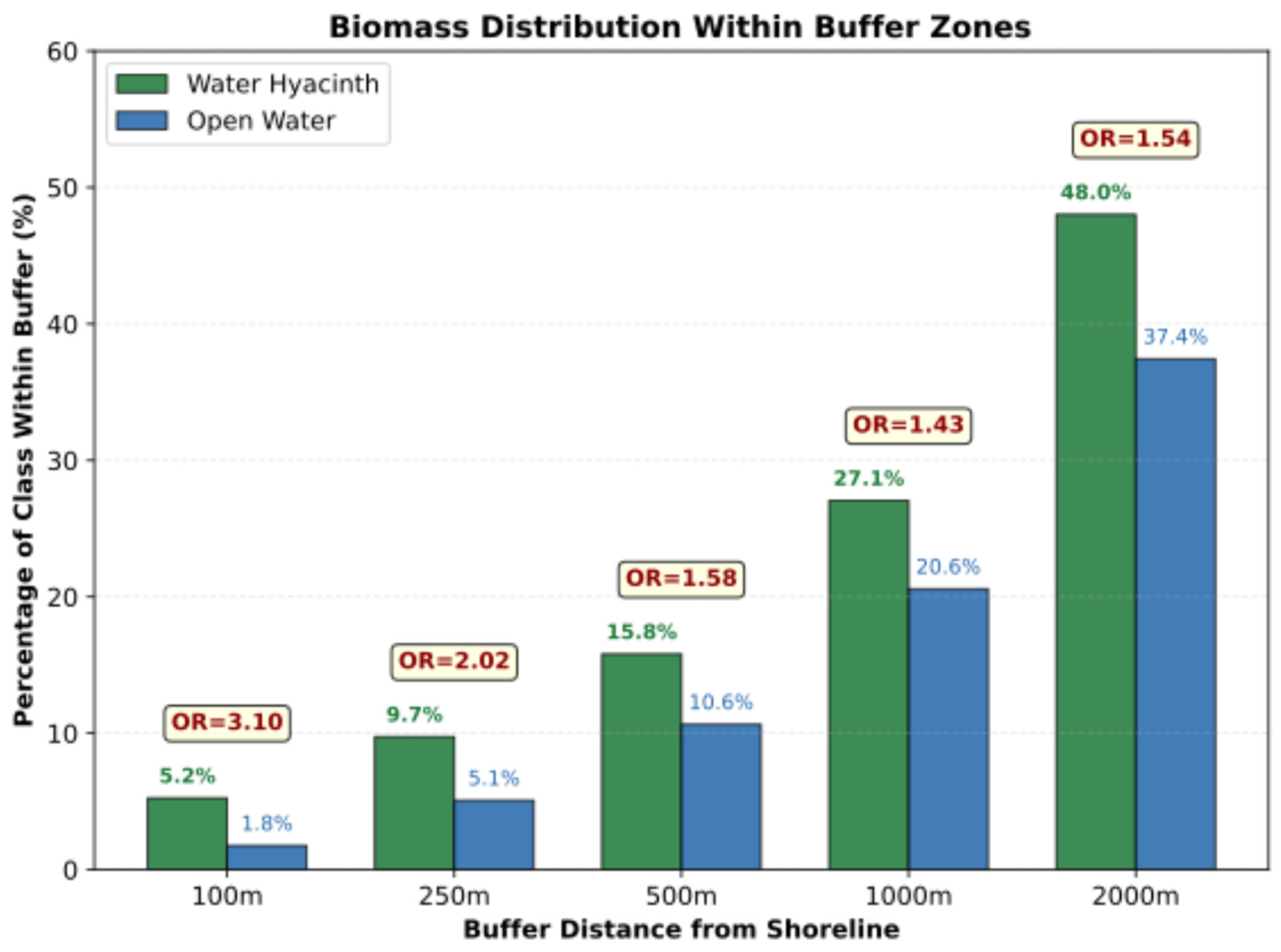
The proportion of water hyacinth pixels within each buffer zone consistently exceeded that of open water, with the disparity most pronounced in near-shore zones (

Table 7. Buffer zone analysis with multiple comparisons correction during peak dry season.

Buffer (m)	Hyacinth Count	Hyacinth (%)	Water (%)	OR	95% CI	χ2	p-Value	Significant?
100	213,153	5.25	1.76	3.10	3.08–3.12	1.37 × 105	<0.001	Yes
250	395,199	9.74	5.08	2.02	2.01–2.03	1.08 × 105	<0.001	Yes
500	641,163	15.80	10.64	1.58	1.57–1.58	7.43 × 104	<0.001	Yes
1000	1,097,889	27.05	20.58	1.43	1.43–1.43	7.14 × 104	<0.001	Yes
2000	1,948,682	48.02	37.44	1.54	1.54–1.55	1.38 × 105	<0.001	Yes

Bonferroni-corrected significance threshold: α = 0.05/5 = 0.01.

). Within 100 m of the shoreline, 5.25% of all water hyacinth pixels were present (n = 213,153), compared to only 1.76% of open water pixels (n = 191,468). This yielded an odds ratio of 3.10 (95% CI: 3.08–3.12), indicating that water hyacinth was approximately three times more likely than open water to occur within 100 m of the shoreline.

At the 2000 m buffer, 48.02% of all water hyacinth biomass was captured (n = 1,948,682), compared to 37.44% of open water (n = 4,078,720), yielding OR = 1.54 (95% CI: 1.54–1.55) (Figure 4).

Percentage of total water hyacinth (green bars) and open water (blue bars) occurring within concentric buffer zones from the shoreline during peak dry season. Values above bars indicate the percentage of class within each buffer zone. Odds ratios (OR) in brown boxes quantify enrichment of water hyacinth relative to open water; OR > 1 indicates preferential nearshore occurrence. Annotation highlights that 48% of total water hyacinth biomass occurs within 2 km of shore (OR = 1.54), compared to 37.4% of open water. Water hyacinth shows the strongest nearshore preference within 100 m (OR = 3.10), indicating approximately three-fold enrichment relative to expected distribution. Preference strength declines systematically with increasing distance but remains significant through a 2000 m buffer (all p < 0.001 after Bonferroni correction, α = 0.01). Pattern supports prioritisation of the 0–500 m zone for mechanical harvesting operations during dry season outbreaks.

3.4.3. Model Comparison and Selection

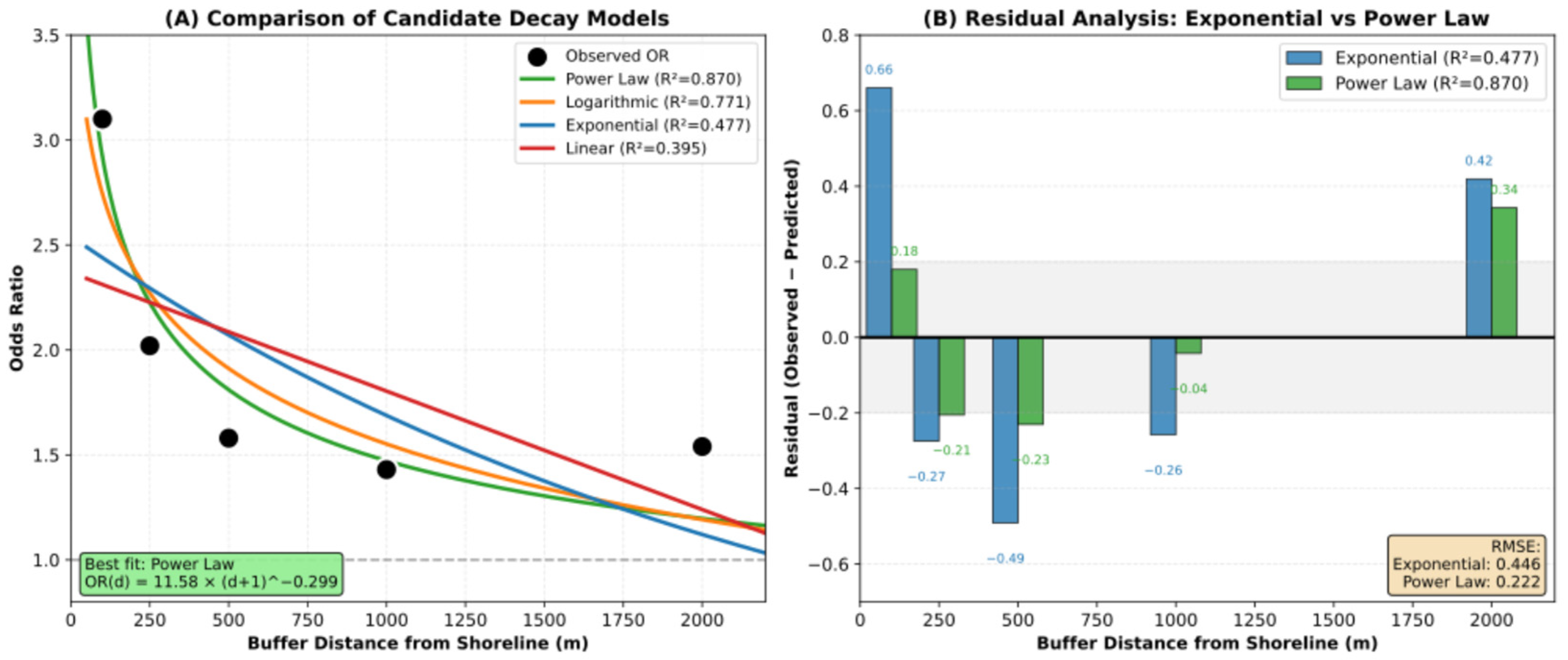
Four candidate models were fitted to the relationship between odds ratio and buffer distance (

Table 8. Comparison of candidate models for shoreline preference decay.

Rank	Model	Formula	R2	AIC	ΔAIC
1	Power Law	OR = a × (d + 1)b	0.870	−11.04	0 (Best)
2	Logarithmic	OR = a + b × ln(d + 1)	0.771	−8.20	+2.84
3	Exponential	OR = a × exp(−b × d)	0.477	−4.07	+6.97
4	Linear	OR = a + b × d	0.395	−3.35	+7.69

). The power law model provided the best empirical fit (R² = 0.870, AIC = −11.04, F = 10.06, p = 0.047), and was the only model achieving overall statistical significance (Figure 5). The exponential (R² = 0.477, AIC = −4.07, F = 1.37, p = 0.378), logarithmic (R² = 0.771, F = 5.05, p = 0.110), and linear (R² = 0.395, F = 0.98, p = 0.471) models all failed to reach significance. Note that with only n = 5 buffer distances and df = 3, p-values have limited power; model selection is therefore based primarily on R² and AIC.

The power law model parameters were as follows (

Table 9. Parameter estimates with bootstrap 95% confidence intervals.

Model	Parameter	Estimate	95% CI	Interpretation
Power Law	a (coefficient)	11.585	1.57–23.31	Scale parameter
	b (exponent)	−0.299	−0.438 to −0.004	Decay exponent
	R2	0.870	—	Variance explained
Exponential	a (initial OR)	2.541	1.48–3.67	OR at shoreline
	b (decay rate)	0.000409 m−1	~0–0.00193	Decay per metre
	Half-distance	1693 m	unstable	Distance for 50% decline
	R2	0.477	—	Variance explained

):

$$OR\left(d\right)=11.585\times (d+1{)}^{-0.299}$$

(16)

3.4.4. Residual Analysis

Residual analysis for the exponential model revealed systematic patterns of misfit (

Table 10. Residual analysis comparing exponential and power law models.

Distance (m)	Observed OR	Exponential Predicted	Exponential Residual	Power Law Predicted	Power Law Residual
100	3.10	2.44	+0.66	2.92	+0.18
250	2.02	2.29	−0.27	2.23	−0.21
500	1.58	2.07	−0.49	1.81	−0.23
1000	1.43	1.69	−0.26	1.47	−0.04
2000	1.54	1.12	+0.42	1.20	+0.34

). The model underestimated odds ratios at the shortest (100 m) and longest (2000 m) distances while overestimating at intermediate distances (500–1000 m).

3.5. Temporal Variability in Shoreline Preference

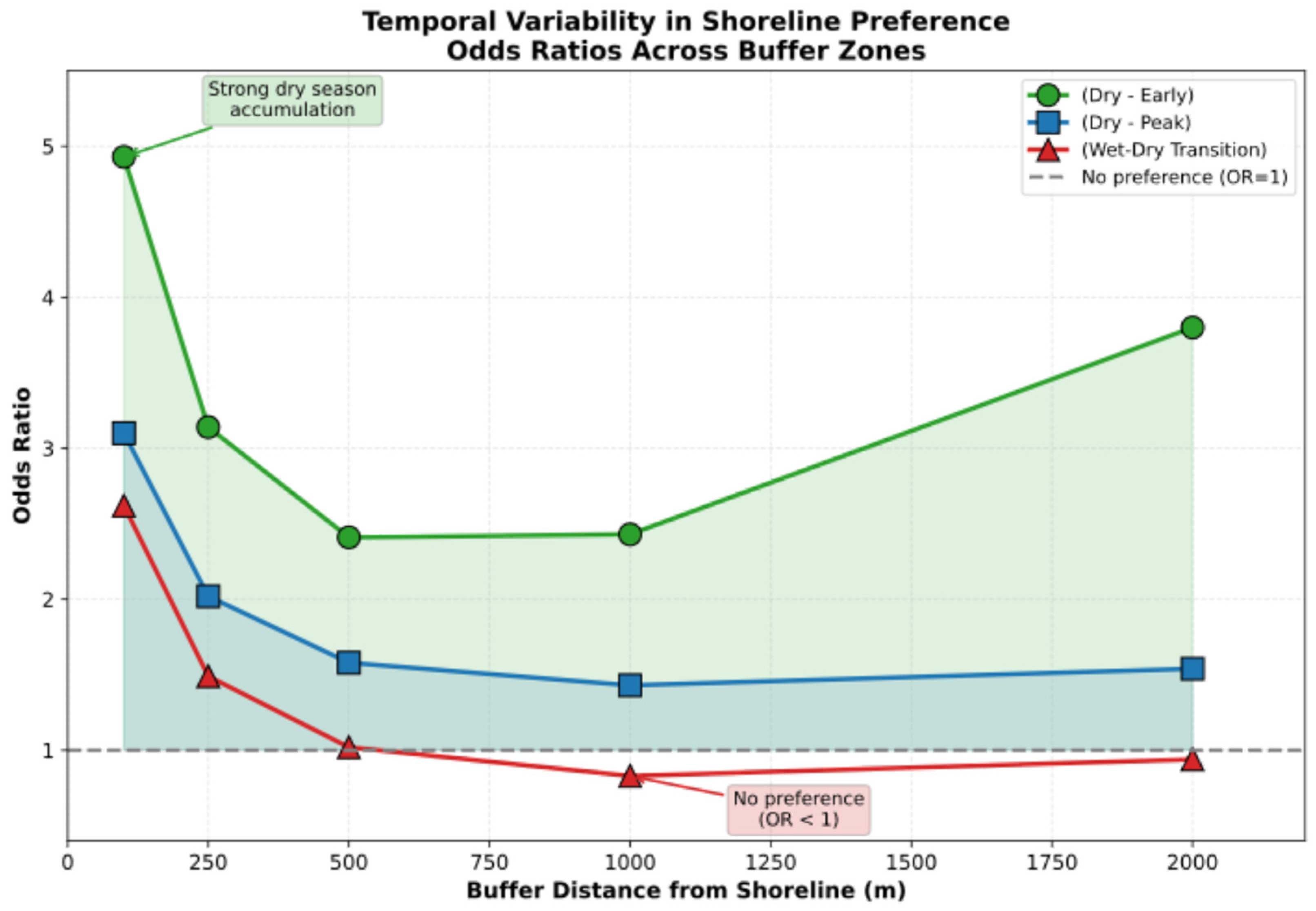
A critical finding of this study is that shoreline preference exhibited substantial temporal variability across seasonal conditions (

Table 11. Temporal variability in shoreline preference across analysis dates.

Season	Preference (m)	95% CI	Cohen’s d	Mann–Whitney p	OR at 100 m	Significant?
Early Dry	+1946.6	+1885 to +2005	0.881	<0.001	4.93	Yes
Peak Dry	+687.9	+617 to +754	0.273	<0.001	3.10	Yes
Wet-Dry Transition	−124.2	−197 to −47	−0.047	1.00	2.62	No

Positive values indicate water hyacinth closer to shore; negative values indicate offshore displacement.

). During both dry season periods, water hyacinth demonstrated significant nearshore accumulation, with preference strengths of +687.9 m (peak dry season; p < 0.001) and +1946.6 m (early dry season; Cohen’s d = 0.881; p < 0.001). In striking contrast, the seasonal transition period revealed a markedly different pattern (

Table 12. Odds ratios by buffer distance across all analysis dates.

Buffer (m)	Early Dry Season	Peak Dry Season	Seasonal Transition
100	4.93	3.10	2.62
250	3.14	2.02	1.49
500	2.41	1.58	1.02
1000	2.43	1.43	0.83
2000	1.85	1.54	0.94

OR > 1 indicates water hyacinth overrepresentation near shore; OR < 1 indicates underrepresentation.

).

During the wet-dry seasonal transition, water hyacinth was distributed slightly farther from shore than open water (preference strength = −124.2 m; 95% CI: −197.4 to −47.0 m). This negative preference was not statistically significant (Mann–Whitney p = 1.00), indicating no evidence of shoreline preference during this period (Figure 6).

4. Discussion

4.1. Spectral Discrimination and Classification Performance

Sentinel-2 MSI provided excellent spectral separability between water hyacinth and open water, with Jeffries–Matusita distances exceeding 1.9 in six of ten bands, substantially above the 1.7 threshold for reliable discrimination [55]. The highest separability occurred in the red (B4; JM = 1.999) and blue (B2; JM = 1.967) bands, reflecting chlorophyll absorption in dense vegetative canopies [81], while pronounced reflectance increases in red edge and NIR regions (mean differences > 2800 units) are characteristic of healthy aquatic macrophytes [23,28]. Moderate separability in green (JM = 0.998) and SWIR2 (JM = 0.756) bands reflected spectral overlap with turbid nearshore water but did not compromise multi-band classification performance [57]. Per-band Shapiro–Wilk tests confirmed approximate normality in 9/10 bands for both classes, supporting the JM distance metric assumptions. Elevated coefficients of variation in hyacinth NIR and red-edge bands (CV = 34–38%) reflect genuine ecological variability in mat density and biomass, rather than measurement error.

Classification accuracy was consistently high across seasons (94–96%; κ = 0.88–0.92), comparing favourably with published water hyacinth mapping studies that typically report 85–95% accuracy [27,28]. The elevated performance likely reflects the polygon-mean sampling approach, which reduces within-class variance [82], the binary classification of spectrally distinct classes [83], and strong inherent separability. Seasonal variation peak dry (96%) outperforming wet-dry transition (94%) likely reflects differences in atmospheric clarity, turbidity, and mat consolidation [36]. Independent validation against NDVI, NDWI, and FAI indices confirmed classification reliability, with the Floating Algae Index showing particularly strong discrimination (difference = +1102), consistent with its design for detecting floating vegetation [26].

4.2. Shoreline Preference and Seasonal Dynamics

While a qualitative tendency for floating macrophytes to accumulate near shorelines is widely acknowledged [9,16], this study provides the first rigorous quantification of that pattern: specific odds ratios, a parameterised decay model, seasonal reversal of preference, and bootstrap confidence intervals that together enable transferable, predictive management. The central finding is that water hyacinth exhibits pronounced but seasonally variable shoreline preference. During dry season conditions, water hyacinth occurred significantly closer to shore than expected under random distribution (preference strengths: +687.9 m peak dry; +1946.6 m early dry; both p < 0.001), while during the wet-dry transition, no significant preference was detected (−124.2 m; p = 1.00). This seasonal modulation challenges assumptions of stable spatial patterns underlying many management approaches. The 687.9 m shoreward displacement during the peak outbreak represents 34.4% of the typical mechanical harvester range (~2000 m from shore; [84]), concentrating harvestable biomass within accessible zones. Buffer zone analysis reinforced this: water hyacinth was 3.10 times more likely than open water to occur within 100 m of shoreline (95% CI: 3.08–3.12), with enrichment declining systematically to OR = 2.02 at 250 m, 1.58 at 500 m, and 1.43 at 1000 m before partially recovering to 1.54 at 2000 m. Critically, 48.0% of total biomass occurred within 2 km of shore compared to 37.4% of open water (all p < 0.001 after Bonferroni correction).

A counterintuitive pattern emerged: early dry season exhibited stronger preference (+1946.6 m; OR at 100 m = 4.93) despite lower total coverage (20.9%) compared to peak dry (+687.9 m; OR = 3.10; coverage = 27.1%). This inverse relationship suggests that nearshore concentration is governed by transport dynamics rather than total abundance. Smaller, fragmented early-season mats may experience more efficient wind-driven transport due to higher surface-area-to-mass ratios and reduced internal friction, enabling rapid shoreward accumulation [42]. As mats grow larger and interconnected, they become increasingly resistant to transport—effectively “anchored” by their own mass—resulting in more dispersed distributions despite higher biomass [45].

The absence of preference during wet-dry transition indicates that wind-driven accumulation mechanisms are either absent or counteracted during this period. Lake Victoria’s wet-dry transition (March–May) is characterized by variable multi-directional winds lacking consistent forcing, elevated rainfall mechanically dispersing mats, higher lake levels altering nearshore hydrodynamics, and stronger riverine inflows potentially pushing vegetation offshore [51].

4.3. Spatial Decay Modelling

The power law function provided substantially superior fit (R² = 0.870; AIC = −11.04; F = 10.06, p = 0.047) to shoreline preference data compared to the theoretically motivated exponential decay model (R² = 0.477; AIC = −4.07; F = 1.37, p = 0.378). The power law was the only model achieving overall statistical significance (p < 0.05), though the low degrees of freedom (df = 3, n = 5 buffer zones) mean model selection rests primarily on R² and AIC rather than p-values alone. This has important implications for understanding governing processes. The exponential model was selected a priori based on wave energy attenuation theory: wave energy in fetch-limited shallow water decays exponentially with distance due to bottom friction and geometric spreading [43,46]. Its failure indicates water hyacinth accumulation dynamics are more complex than simple wave attenuation predicts. The power law model OR(d) = 11.585 × (d + 1)^−0.299 implies a rapid initial decline within the first few hundred metres followed by a gradual plateau at intermediate distances. Power law relationships commonly arise when multiple interacting processes operate across scales [49,50], and the superior fit may reflect superposition of wave-driven transport, depth-mediated settling, nutrient gradients, and physical barriers operating at different spatial scales. Residual analysis confirmed exponential model inadequacy: systematic underestimation at extremes (100 m: residual = +0.66; 2000 m: +0.42) and overestimation at intermediate distances (500–1000 m: −0.26 to −0.49), while power law residuals showed no systematic pattern (−0.23 to +0.34). However, only five buffer distances were analysed, limiting discrimination among functional forms. The power law may provide better empirical fit without necessarily representing the “true” underlying process. Future analyses incorporating additional buffer distances would strengthen model selection and parameter uncertainty estimation.

4.4. Hydrodynamic Mechanisms

The seasonal patterns can be explained by contrasting hydrodynamic regimes. During dry season (June–October), persistent southeasterly trade winds generate surface waves propagating toward northern and western shorelines [51], creating three interacting accumulation mechanisms. First, surface waves generate Stokes drift net mass transport in the wave propagation direction producing persistent shoreward displacement of floating objects [44,45]. For water hyacinth mats with high surface-area-to-draft ratios, Stokes drift produces substantial cumulative transport over days to weeks. Second, wave energy dissipation in shallow water creates distinct zones: offshore (>2 km) where sustained turbulence disperses mats; transition (500–2000 m) where declining energy permits coalescence; and nearshore (<500 m) where rapid dissipation enables stable accumulation [47]. This explains the 15.8% biomass concentration within 500 m (OR = 1.58). Third, nutrient gradients from riverine and urban sources may enhance nearshore growth rates [52], though rapid seasonal reversal of preference patterns suggests physical transport dominates.

During wet season and wet-dry transition (March–May), these mechanisms are disrupted: variable winds eliminate consistent forcing, elevated rainfall disturbs mats and increases turbidity, higher lake levels alter hydrodynamic zones, and stronger riverine inflows create offshore-pushing plumes [52].

4.5. Management Implications

The findings support adaptive, seasonally adjusted management strategies. During dry season (June–October), mechanical harvesting should prioritize nearshore zones where biomass is disproportionately concentrated, achieving higher removal efficiency per unit effort [10]. During wet season transitions (March–May), when shoreline preference is absent, broader surveillance and opportunistic removal of large aggregations regardless of location may be more appropriate.

A three-tiered priority framework is recommended based on buffer zone analysis. The priority zone (0–500 m) exhibited the strongest enrichment (OR = 1.58–3.10), warranting intensive monitoring and harvesting during dry season outbreaks, with the 100 m nearshore strip representing the highest-priority target (OR = 3.10). The secondary zone (500–2000 m) showed moderate enrichment (OR = 1.43–1.54) containing 48% of total biomass within 2 km of shore; routine management should target this zone when capacity permits. The tertiary zone (>2000 m) contains water hyacinth at near-random distribution; intervention should focus on persistent large mats serving as propagule sources for nearshore reinfestation.

The power law model OR(d) = 11.585 × (d + 1)^−0.299 enables predictive estimation of enrichment at any distance during the dry season (e.g., 300 m: OR ≈ 2.3; 750 m: OR ≈ 1.6; 1500 m: OR ≈ 1.3), informing spatial prioritization of limited resources. The stronger early dry season preference (+1946.6 m) despite lower coverage (20.9%) suggests early intervention may be particularly efficient: smaller biomass more concentrated nearshore enables removal before mats grow and disperse. This supports aggressive early dry season intervention followed by sustained effort through peak dry season, rather than waiting for peak biomass accumulation when spatial concentration weakens.

4.6. Limitations and Future Research

Several limitations warrant consideration. First, the absence of high-resolution bathymetric data prevents partitioning depth from distance effects. Nearshore zones are systematically shallower (<3 m) than offshore areas (>5 m); observed “shoreline preference” may partially reflect “shallow water preference” where reduced wave velocities, potential substrate anchoring, and nutrient-rich sediments enhance stability regardless of horizontal distance [51]. The power law pattern may itself reflect bathymetric gradients if shallow shelves extend offshore. Second, Euclidean distance assumes isotropic transport with equal probability in all directions. Water hyacinth transport is actually anisotropic, governed by wind vectors, wave directions, and currents varying spatially and temporally [42]. Cost-distance metrics incorporating directional transport would provide more realistic “functional distance” estimates but were beyond this study’s scope. Third, the study does not include imagery from the true wet season (March–May); the wet–dry transition image (31 May 2020) captures only the tail of that period and cannot fully represent peak-rainfall hydrodynamics, when lake levels, riverine discharge, and multi-directional winds differ most from dry-season conditions. A future study spanning complete annual cycles would be needed to confirm whether wet-season spatial patterns are systematically different. Fourth, temporal analysis encompassed only three dates across 2020. Lake Victoria has experienced substantial inter-annual fluctuations in water hyacinth abundance driven by ENSO cycles, nutrient loading, biological control effectiveness, and management intensity [16,36]. Patterns documented here may not generalize to years with different climate forcing or baseline infestation levels. Fourth, model fitting relied on only five buffer distances, limiting discrimination among functional forms. With additional data points at finer resolution, alternative or multi-phase models might prove superior. Finally, while classification accuracy was high (94–96%), misclassification errors are non-randomly distributed, predominantly at class boundaries, sparse vegetation areas, and high-turbidity zones. This spatial non-randomness could bias buffer statistics, though the direction is difficult to predict without explicit error modelling.

Future research priorities include: (1) integrating bathymetric data to partition depth and distance effects and test alternative accumulation hypotheses; (2) multi-year seasonal analysis spanning different ENSO phases and management intensities to assess pattern robustness; (3) coupling distribution data with hydrodynamic models incorporating wind, waves, and currents to mechanistically test transport hypotheses using Lagrangian particle tracking; (4) comparing windward versus lee shore accumulation patterns to validate wind-driven transport mechanisms; and (5) developing automated classification systems for near-real-time monitoring and early warning to support adaptive management.

5. Conclusions

Based on three temporally contrasting Sentinel-2 images representing distinct seasonal hydrodynamic regimes within 2020, this study provides the first quantitative assessment of water hyacinth shoreline preference in Lake Victoria. The findings indicate that spatial dynamics are strongly modulated by seasonal hydrodynamic conditions, though multi-year validation will be needed to confirm the generalisability of these patterns across interannual variability. High-resolution satellite imagery enabled reliable discrimination of floating mats from open water, establishing a robust methodological framework for monitoring and mapping. The results demonstrate that water hyacinth does not maintain a constant spatial pattern but instead exhibits marked nearshore accumulation during dry season conditions, driven by wind- and wave-induced transport, while distribution becomes more dispersed and unpredictable during transitional periods. The distance-dependent decay of shoreline preference follows a non-linear pattern, reflecting the interaction of bathymetry, wave energy, and hydrodynamic processes rather than simple exponential decline. These insights highlight the critical role of temporal and environmental context in understanding and managing invasive aquatic vegetation, providing a strong foundation for adaptive management strategies that target high-priority nearshore zones during periods of maximal accumulation while acknowledging the limitations of spatial targeting under dispersive conditions. Overall, the study underscores the importance of integrating remote sensing, spatial modelling, and ecological understanding to inform evidence-based management of persistent invasive species.

References

1. Holm, L.G.; Plucknett, D.L.; Pancho, J.V.; Herberger, J.P. The World’s Worst Weeds: Distribution and Biology; University Press of Hawaii: Honolulu, HI, USA, 1977. [Google Scholar]
2. Téllez, T.R.; López, E.M.; Granado, G.L.; Pérez, E.A.; López, R.M.; Guzmán, J.M.S. The water hyacinth, Eichhornia crassipes: An invasive plant in the Guadiana River Basin (Spain). Aquat. Invasions 2008, 3, 42–53. [Google Scholar] [CrossRef]
3. Villamagna, A.M.; Murphy, B.R. Ecological and socio-economic impacts of invasive water hyacinth (Eichhornia crassipes): A review. Freshw. Biol. 2010, 55, 282–298. [Google Scholar] [CrossRef]
4. Coetzee, J.A.; Hill, M.P.; Byrne, M.J.; Bownes, A. A review of the biological control programmes on Eichhornia crassipes (C.Mart.) Solms (Pontederiaceae), Salvinia molesta D.S.Mitch. (Salviniaceae), Pistia stratiotes L. (Araceae), Myriophyllum aquaticum (Vell.) Verdc. (Haloragaceae) and Azolla filiculoides Lam. (Azollaceae) in South Africa. Afr. Entomol. 2011, 19, 451–468. [Google Scholar] [CrossRef]
5. Reddy, K.R.; Tucker, J.C. Productivity and nutrient uptake of water hyacinth, Eichhornia crassipes: I. Effect of nitrogen source. Econ. Bot. 1983, 37, 237–247. [Google Scholar] [CrossRef]
6. Malik, A. Environmental challenge vis-a-vis opportunity: The case of water hyacinth. Environ. Int. 2007, 33, 122–138. [Google Scholar] [CrossRef]
7. Masifwa, W.F.; Twongo, T.; Denny, P. The impact of water hyacinth, Eichhornia crassipes (Mart) Solms on the abundance and diversity of aquatic macroinvertebrates along the shores of northern Lake Victoria, Uganda. Hydrobiologia 2001, 452, 79–88. [Google Scholar] [CrossRef]
8. Scheffer, M.; Rinaldi, S.; Gragnani, A.; Mur, L.R.; van Nes, E.H. On the dominance of filamentous cyanobacteria in shallow, turbid lakes. Ecology 1997, 78, 272–282. [Google Scholar] [CrossRef]
9. Kateregga, E.; Sterner, T. Lake Victoria fish stocks and the effects of water hyacinth. J. Environ. Dev. 2009, 18, 62–78. [Google Scholar] [CrossRef]
10. Güereña, D.; Neuenschwander, P.; Jucker, C. Economic Impact of Water Hyacinth on Lake Victoria and Policy Options for Control; CABI Working Paper No. 8; CAB International: Wallingford, UK, 2015. [Google Scholar]
11. Twongo, T.; Bugenyi, F.W.B.; Wanda, F. The potential for further proliferation of water hyacinth in lakes Victoria, Kyoga and Kwania and some urgent aspects for research. Afr. J. Trop. Hydrobiol. Fish. 1995, 6, 1–10. [Google Scholar] [CrossRef]
12. Hecky, R.E.; Mugidde, R.; Ramlal, P.S.; Talbot, M.R.; Kling, G.W. Multiple stressors cause rapid ecosystem change in Lake Victoria. Freshw. Biol. 2010, 55, 19–42. [Google Scholar] [CrossRef]
13. Nyamweya, C.; Lawrence, T.J.; Ajode, M.Z.; Smith, S.; Achieng, A.O.; Barasa, J.E.; Masese, F.O.; Taabu-Munyaho, A.; Mahongo, S.; Kayanda, R.; et al. Lake Victoria: Overview of research needs and the way forward. J. Great Lakes Res. 2023, 49, 102211. [Google Scholar] [CrossRef]
14. Gichuki, J.; Omondi, R.; Boera, P.; Okorut, T.; Matano, A.S.; Jembe, T.; Ofulla, A. Water hyacinth Eichhornia crassipes (Mart.) Solms-Laubach dynamics and succession in the Nyanza Gulf of Lake Victoria (East Africa): Implications for water quality and biodiversity conservation. Sci. World J. 2012, 2012, 106429. [Google Scholar] [CrossRef]
15. Njagi, D.M.; Routh, J.; Odhiambo, M.; Luo, C.; Basapuram, L.G.; Olago, D.; Klump, V.; Stager, C. A century of human-induced environmental changes and the combined roles of nutrients and land use in Lake Victoria catchment on eutrophication. Sci. Total Environ. 2022, 835, 155425. [Google Scholar] [CrossRef] [PubMed]
16. Albright, T.P.; Moorhouse, T.G.; McNabb, T.J. The rise and fall of water hyacinth in Lake Victoria and the Kagera River Basin, 1989–2001. J. Aquat. Plant Manag. 2004, 42, 73–84. [Google Scholar]
17. Neuenschwander, P.; Julien, M.H.; Center, T.D.; Hill, M.P. Pistia stratiotes L. (Araceae). In Biological Control of Tropical Weeds Using Arthropods; Muniappan, R., Reddy, G.V.P., Raman, A., Eds.; Cambridge University Press: Cambridge, UK, 2009; pp. 332–352. [Google Scholar] [CrossRef]
18. Felix, I.K.; Marino, A.; Simpson, M.D.; Akbari, V.; Silva, T.S.F.; Datta, A.; Nagendra, P.G.; Pranuthi, G.; Srikanth, R. Mapping and monitoring of water hyacinth in Lake Victoria using polarimetric radar data. IEEE J. Sel. Top. Appl. Earth Obs. Remote Sens. 2024, 17, 19900–19910. [Google Scholar] [CrossRef]
19. Silva, T.S.F.; Costa, M.P.F.; Melack, J.M.; Novo, E.M.L.M. Remote sensing of aquatic vegetation: Theory and applications. Environ. Monit. Assess. 2007, 140, 131–145. [Google Scholar] [CrossRef]
20. Hestir, E.L.; Brando, V.E.; Bresciani, M.; Giardino, C.; Matta, E.; Villa, P.; Dekker, A.G. Measuring freshwater aquatic ecosystems: The need for a hyperspectral global mapping satellite mission. Remote Sens. Environ. 2015, 167, 181–195. [Google Scholar] [CrossRef]
21. Stratoulias, D.; Balzter, H.; Sykioti, O.; Zlinszky, A.; Tóth, V.R. Evaluating Sentinel-2 for lakeshore habitat mapping based on airborne hyperspectral data. Sensors 2015, 15, 22956–22969. [Google Scholar] [CrossRef]
22. Jensen, J.R. Remote Sensing of the Environment: An Earth Resource Perspective, 2nd ed.; Pearson Prentice Hall: Upper Saddle River, NJ, USA, 2007. [Google Scholar]
23. Villa, P.; Laini, A.; Bresciani, M.; Bolpagni, R. A remote sensing approach to monitor the conservation status of lacustrine Phragmites australis beds. Wetl. Ecol. Manag. 2013, 23, 35–49. [Google Scholar] [CrossRef]
24. Rouse, J.W.; Haas, R.H.; Schell, J.A.; Deering, D.W. Monitoring vegetation systems in the Great Plains with ERTS. In Proceedings of the Third Earth Resources Technology Satellite-1 Symposium, NASA SP-351, Greenbelt, MD, USA, 10–14 December 1973; pp. 309–317. [Google Scholar]
25. McFeeters, S.K. The use of the Normalized Difference Water Index (NDWI) in the delineation of open water features. Int. J. Remote Sens. 1995, 17, 1425–1432. [Google Scholar] [CrossRef]
26. Hu, C. A novel ocean color index to detect floating algae in the global oceans. Remote Sens. Environ. 2009, 113, 2118–2129. [Google Scholar] [CrossRef]
27. Dube, T.; Mutanga, O.; Sibanda, M.; Bangamwabo, V.; Shoko, C. Evaluating the performance of the newly-launched Landsat 8 sensor in detecting and mapping the spatial configuration of water hyacinth (Eichhornia crassipes) in inland lakes, Zimbabwe. Phys. Chem. Earth 2017, 100, 101–111. [Google Scholar] [CrossRef]
28. Thamaga, K.H.; Dube, T. Remote sensing of invasive water hyacinth (Eichhornia crassipes): A review on applications and challenges. Remote Sens. Appl. Soc. Environ. 2018, 10, 36–46. [Google Scholar] [CrossRef]
29. Ruwaimana, M.; Satyanarayana, B.; Otero, V.; Muslim, A.M.; Syafiq, A.M.; Ibrahim, S.; Raymaekers, D.; Koedam, N.; Dahdouh-Guebas, F. The advantages of using drones over space-borne imagery in the mapping of mangrove forests. PLoS ONE 2018, 13, e0200288. [Google Scholar] [CrossRef]
30. Mudereri, B.T.; Dube, T.; Niassy, S.; Kimathi, E.; Landmann, T.; Khan, Z.; Abdel-Rahman, E.M. A comparative analysis of PlanetScope and Sentinel-2 space-borne sensors in mapping Striga weed using Guided Regularised Random Forest classification ensemble. ISPRS Ann. 2019, XLII-2/W13, 701–708. [Google Scholar] [CrossRef]
31. Rodríguez-Garlito, E.C.; Paz-Gallardo, A.; Plaza, A. Mapping invasive aquatic plants in Sentinel-2 images using convolutional neural networks trained with spectral indices. IEEE J. Sel. Top. Appl. Earth Obs. Remote Sens. 2023, 16, 2889–2899. [Google Scholar] [CrossRef]
32. Pirbasti, M.A.; Akbari, V.; Bhowmik, D.; Maharaj, S.; Marino, A. Detection and mapping of water hyacinth growth cycle in Anzali International Wetland using Sentinel-2 time series. IEEE J. Sel. Top. Appl. Earth Obs. Remote Sens. 2024, 17, 13346–13357. [Google Scholar] [CrossRef]
33. Damtie, Y.A.; Mengistu, D.A.; Meshesha, D.T. Spatial coverage of water hyacinth (Eichhornia crassipes (Mart.) Solms) on Lake Tana and associated water loss. Heliyon 2021, 7, e08196. [Google Scholar] [CrossRef] [PubMed]
34. Nininahazwe, F.; Théau, J.; Genest, M.A.; Varin, M. Mapping invasive alien plant species with very high spatial resolution and multi-date satellite imagery using object-based and machine learning techniques: A comparative study. GIScience Remote Sens. 2023, 60, 2190203. [Google Scholar] [CrossRef]
35. Thamaga, K.H.; Dube, T. Understanding seasonal dynamics of invasive water hyacinth (Eichhornia crassipes) in the Greater Letaba river system using Sentinel-2 satellite data. GIScience Remote Sens. 2019, 56, 1355–1377. [Google Scholar] [CrossRef]
36. Fusilli, L.; Collins, M.O.; Laneve, G.; Palombo, A.; Pignatti, S.; Santini, F. Assessment of the abnormal growth of floating macrophytes in Winam Gulf (Kenya) by using MODIS imagery time series. Int. J. Appl. Earth Obs. Geoinf. 2013, 20, 33–41. [Google Scholar] [CrossRef]
37. Drusch, M.; Del Bello, U.; Carlier, S.; Colin, O.; Fernandez, V.; Gascon, F.; Hoersch, B.; Isola, C.; Laberinti, P.; Martimort, P.; et al. Sentinel-2: ESA’s optical high-resolution mission for GMES operational services. Remote Sens. Environ. 2012, 120, 25–36. [Google Scholar] [CrossRef]
38. European Space Agency. Sentinel-2 User Handbook; ESA Standard Document; ESA: Paris, France, 2015; Available online: https://sentinels.copernicus.eu/documents/247904/685211/Sentinel-2_User_Handbook (accessed on 28 January 2026).
39. Clevers, J.G.P.W.; Gitelson, A.A. Remote estimation of crop and grass chlorophyll and nitrogen content using red-edge bands on Sentinel-2 and -3. Int. J. Appl. Earth Obs. Geoinf. 2013, 23, 344–351. [Google Scholar] [CrossRef]
40. Toming, K.; Kutser, T.; Laas, A.; Sepp, M.; Paavel, B.; Nõges, T. First experiences in mapping lake water quality parameters with Sentinel-2 MSI imagery. Remote Sens. 2016, 8, 640. [Google Scholar] [CrossRef]
41. Blaschke, T. Object based image analysis for remote sensing. ISPRS J. Photogramm. Remote Sens. 2010, 65, 2–16. [Google Scholar] [CrossRef]
42. Verhagen, J.H.G.; Nienhuis, P.H. A simulation model of production, seasonal changes in biomass and distribution of eelgrass (Zostera marina) in Lake Grevelingen. Mar. Ecol. Prog. Ser. 1983, 10, 187–195. [Google Scholar] [CrossRef]
43. Young, I.R.; Verhagen, L.A. The growth of fetch limited waves in water of finite depth. Part 1. Total energy and peak frequency. Coast. Eng. 1996, 29, 47–78. [Google Scholar] [CrossRef]
44. Stokes, G.G. On the theory of oscillatory waves. Trans. Camb. Philos. Soc. 1847, 8, 441–455. [Google Scholar]
45. van den Bremer, T.S.; Breivik, Ø. Stokes drift. Philos. Trans. R. Soc. A 2018, 376, 20170104. [Google Scholar] [CrossRef]
46. Booij, N.; Ris, R.C.; Holthuijsen, L.H. A third-generation wave model for coastal regions: 1. Model description and validation. J. Geophys. Res. Ocean 1999, 104, 7649–7666. [Google Scholar] [CrossRef]
47. Pomeroy, A.W.M.; Lowe, R.J.; Symonds, G.; Van Dongeren, A.R.; Moore, C. The dynamics of infragravity wave transformation over a fringing reef. J. Geophys. Res. Ocean 2012, 117, C11022. [Google Scholar] [CrossRef]
48. MacIntyre, S.; Romero, J.R.; Silsbe, G.M.; Emery, B.M. Stratification and horizontal exchange in Lake Victoria, East Africa. Limnol. Oceanogr. 2014, 59, 1805–1838. [Google Scholar] [CrossRef]
49. Clauset, A.; Shalizi, C.R.; Newman, M.E.J. Power-law distributions in empirical data. SIAM Rev. 2009, 51, 661–703. [Google Scholar] [CrossRef]
50. Newman, M.E.J. Power laws, Pareto distributions and Zipf’s law. Contemp. Phys. 2005, 46, 323–351. [Google Scholar] [CrossRef]
51. Okely, P.; Imberger, J.; Antenucci, J.P. Processes affecting horizontal mixing and dispersion in Winam Gulf, Lake Victoria. Limnol. Oceanogr. 2010, 55, 1865–1880. [Google Scholar] [CrossRef]
52. Gikuma-Njuru, P.; Hecky, R.E.; Guildford, S.J.; MacIntyre, S. Spatial variability of nutrient concentrations, fluxes, and ecosystem metabolism in Nyanza Gulf and Rusinga Channel, Lake Victoria (East Africa). Limnol. Oceanogr. 2013, 58, 774–789. [Google Scholar] [CrossRef]
53. Main-Knorn, M.; Pflug, B.; Louis, J.; Debaecker, V.; Müller-Wilm, U.; Gascon, F. Sen2Cor for Sentinel-2. Proc. SPIE 2017, 10427, 1042704. [Google Scholar] [CrossRef]
54. Bruzzone, L.; Roli, F.; Serpico, S.B. An extension of the Jeffreys-Matusita distance to multiclass cases for feature selection. IEEE Trans. Geosci. Remote Sens. 1995, 33, 1318–1321. [Google Scholar] [CrossRef]
55. Richards, J.A.; Jia, X. Remote Sensing Digital Image Analysis: An Introduction, 4th ed.; Springer: Berlin, Germany, 2006. [Google Scholar] [CrossRef]
56. Vapnik, V. The Nature of Statistical Learning Theory; Springer: New York, NY, USA, 1995. [Google Scholar] [CrossRef]
57. Mountrakis, G.; Im, J.; Ogole, C. Support vector machines in remote sensing: A review. ISPRS J. Photogramm. Remote Sens. 2011, 66, 247–259. [Google Scholar] [CrossRef]
58. Sheykhmousa, M.; Mahdianpari, M.; Ghanbari, H.; Mohammadimanesh, F.; Ghamisi, P.; Homayouni, S. Support vector machine versus random forest for remote sensing image classification: A meta-analysis and systematic review. IEEE J. Sel. Top. Appl. Earth Obs. Remote Sens. 2020, 13, 6308–6325. [Google Scholar] [CrossRef]
59. Belgiu, M.; Drăguţ, L. Random forest in remote sensing: A review of applications and future directions. ISPRS J. Photogramm. Remote Sens. 2016, 114, 24–31. [Google Scholar] [CrossRef]
60. Ma, L.; Li, M.; Ma, X.; Cheng, L.; Du, P.; Liu, Y. A review of supervised object-based land-cover image classification. ISPRS J. Photogramm. Remote Sens. 2017, 130, 277–293. [Google Scholar] [CrossRef]
61. Congalton, R.G.; Green, K. Assessing the Accuracy of Remotely Sensed Data: Principles and Practices, 3rd ed.; CRC Press: Boca Raton, FL, USA, 2019. [Google Scholar] [CrossRef]
62. Foody, G.M. Status of land cover classification accuracy assessment. Remote Sens. Environ. 2002, 80, 185–201. [Google Scholar] [CrossRef]
63. Snyder, J.P. Map Projections: A Working Manual; U.S. Geological Survey Professional Paper 1395; U.S. Government Printing Office: Washington, DC, USA, 1987. [Google Scholar] [CrossRef]
64. Virtanen, P.; Gommers, R.; Oliphant, T.E.; Haberland, M.; Reddy, T.; Cournapeau, D.; Burovski, E.; Peterson, P.; Weckesser, W.; Bright, J.; et al. SciPy 1.0 Contributors. SciPy 1.0: Fundamental algorithms for scientific computing in Python. Nat. Methods 2020, 17, 261–272. [Google Scholar] [CrossRef]
65. Sokal, R.R.; Rohlf, F.J. Biometry: The Principles and Practice of Statistics in Biological Research, 3rd ed.; W.H. Freeman: New York, NY, USA, 1995. [Google Scholar]
66. Efron, B.; Tibshirani, R.J. An Introduction to the Bootstrap; Chapman & Hall: New York, NY, USA, 1993. [Google Scholar] [CrossRef]
67. Mann, H.B.; Whitney, D.R. On a test of whether one of two random variables is stochastically larger than the other. Ann. Math. Stat. 1947, 18, 50–60. [Google Scholar] [CrossRef]
68. Wilcox, R.R. Fundamentals of Modern Statistical Methods: Substantially Improving Power and Accuracy, 2nd ed.; Springer: New York, NY, USA, 2010. [Google Scholar] [CrossRef]
69. Agresti, A. Categorical Data Analysis, 2nd ed.; John Wiley & Sons: Hoboken, NJ, USA, 2002. [Google Scholar] [CrossRef]
70. Bland, J.M.; Altman, D.G. Multiple significance tests: The Bonferroni method. BMJ 1995, 310, 170. [Google Scholar] [CrossRef] [PubMed]
71. Moré, J.J. The Levenberg-Marquardt algorithm: Implementation and theory. In Numerical Analysis; Watson, G.A., Ed.; Lecture Notes in Mathematics; Springer: Berlin, Germany, 1978; Volume 630, pp. 105–116. [Google Scholar] [CrossRef]
72. Akaike, H. A new look at the statistical model identification. IEEE Trans. Autom. Control 1974, 19, 716–723. [Google Scholar] [CrossRef]
73. Burnham, K.P.; Anderson, D.R. Model Selection and Multimodel Inference: A Practical Information-Theoretic Approach, 2nd ed.; Springer: New York, NY, USA, 2002. [Google Scholar]
74. Van Rossum, G.; Drake, F.L. Python 3 Reference Manual; CreateSpace: Scotts Valley, CA, USA, 2009. [Google Scholar]
75. Gillies, S.; van der Walt, S.; Dale, D. Rasterio: Geospatial Raster I/O for Python Programmers; Zenodo: Geneva, Switzerland, 2020; Available online: https://rasterio.readthedocs.io/en/stable/ (accessed on 4 April 2025).
76. Jordahl, K.; Van den Bossche, J.; Fleischmann, M.; Wasserman, J.; McBride, J.; Gerard, J.; Tratner, J.; Perry, M.; Garcia Badaracco, A.; Farmer, C.; et al. geopandas/geopandas, version 0.8.1; Zenodo: Geneva, Switzerland, 2020. [Google Scholar] [CrossRef]
77. Pedregosa, F.; Varoquaux, G.; Gramfort, A.; Michel, V.; Thirion, B.; Grisel, O.; Blondel, M.; Prettenhofer, P.; Weiss, R.; Dubourg, V.; et al. Scikit-learn: Machine learning in Python. J. Mach. Learn. Res. 2011, 12, 2825–2830. [Google Scholar]
78. Harris, C.R.; Millman, K.J.; van der Walt, S.J.; Gommers, R.; Virtanen, P.; Cournapeau, D.; Wieser, E.; Taylor, J.; Berg, S.; Smith, N.J.; et al. Array programming with NumPy. Nature 2020, 585, 357–362. [Google Scholar] [CrossRef] [PubMed]
79. Hunter, J.D. Matplotlib: A 2D graphics environment. Comput. Sci. Eng. 2007, 9, 90–95. [Google Scholar] [CrossRef]
80. Waskom, M. seaborn: Statistical data visualization. J. Open Source Softw. 2021, 6, 3021. [Google Scholar] [CrossRef]
81. Gitelson, A.A.; Gritz, Y.; Merzlyak, M.N. Relationships between leaf chlorophyll content and spectral reflectance and algorithms for non-destructive chlorophyll assessment in higher plant leaves. J. Plant Physiol. 2003, 160, 271–282. [Google Scholar] [CrossRef]
82. Duro, D.C.; Franklin, S.E.; Dubé, M.G. A comparison of pixel-based and object-based image analysis with selected machine learning algorithms for the classification of agricultural landscapes using SPOT-5 HRG imagery. Remote Sens. Environ. 2012, 118, 259–272. [Google Scholar] [CrossRef]
83. Foody, G.M.; Mathur, A. Toward intelligent training of supervised image classifications: Directing training data acquisition for SVM classification. Remote Sens. Environ. 2004, 93, 107–117. [Google Scholar] [CrossRef]
84. Ongore, C.O.; Aura, C.M.; Ogari, Z.; Njiru, J.M.; Nyamweya, C.S. Spatial-temporal dynamics of water hyacinth, Eichhornia crassipes (Mart.) and other macrophytes and their impact on fisheries in Lake Victoria, Kenya. J. Great Lakes Res. 2018, 44, 1273–1280. [Google Scholar] [CrossRef]
Figure 1. Location of Winam Gulf study area within Lake Victoria, East Africa. (A) Main map shows Winam Gulf in northeastern Lake Victoria, Kenya; (B) upper-right inset shows the regional context in East Africa; (C) lower-right inset shows Kenya’s location in Africa.
Limnolrev 26 00024 g001
Figure 2. Classified water hyacinth distribution during peak dry season with shoreline buffer zones.
Limnolrev 26 00024 g002
Figure 3. Spatial distributions and temporal variability of water hyacinth distance to shoreline. (A) Probability density of water hyacinth (green) and open water (blue) shows hyacinth concentrated nearshore. (B) Seasonal box plots indicate closer shoreline association of hyacinth during the dry season. (C) Cumulative distributions highlight 50% hyacinth coverage at shorter distances from shore than open water. (D) Seasonal variation in preference strength shows strongest nearshore association during the dry season.
Limnolrev 26 00024 g003
Figure 4. Biomass distribution of water hyacinth and open water within nearshore buffer zones.
Limnolrev 26 00024 g004
Figure 5. (A) Observed shoreline preference of water hyacinth during peak dry season compared with four candidate spatial decay models; the power law (green) provides the best fit, capturing rapid nearshore decay and gradual plateau. (B) Residuals for exponential (blue) and power law (green) models show the power law has smaller, non-systematic deviations, confirming superior fit.
Limnolrev 26 00024 g005
Figure 6. Seasonal variation in shoreline preference across buffer zones. Temporal variation in shoreline preference of water hyacinth across three seasonal periods. Early dry season shows strongest nearshore enrichment, peak dry season moderate preference, and seasonal transition weak or absent preference, indicating seasonal modulation of shoreline association. Line colors represent seasonal periods; dashed line indicates odds ratio = 1 (no shoreline preference).
Limnolrev 26 00024 g006