Article

Numerical Solutions of Nonlinear Delay Mixed Integral Equation in Two Dimensions via Collocation Method Based on Chebyshev and Legendre Polynomials


Department of Mathematics, College of Science, Taif University, P.O. Box 11099, Taif 21944, Saudi Arabia
*
Author to whom correspondence should be addressed.
Math. Comput. Appl. 2026, 31(2), 59; https://doi.org/10.3390/mca31020059
Submission received: 22 January 2026 / Revised: 31 March 2026 / Accepted: 7 April 2026 / Published: 9 April 2026
(This article belongs to the Section Natural Sciences)

Abstract

This research investigates the numerical analysis of a two-dimensional (2D) delay mixed integral equation (DMIE) of the second kind with a continuous kernel. The existence, uniqueness, stability, and convergence of the solution are rigorously established in the functional space C ( [ a , b ] × [ 0 , T ] ) , providing a solid theoretical foundation. A collocation method based on Chebyshev and Legendre polynomials is applied to obtain accurate numerical approximations, leading to a system of algebraic equations applicable to both linear and nonlinear cases. Numerical simulations are performed using MATLAB to evaluate the method’s performance and calculate the results, including error behavior, convergence, and stability. Several illustrative applications are presented to demonstrate the method’s numerical stability and versatility in handling both linear and nonlinear problems. The results underscore the efficiency, accuracy, and robustness of the proposed numerical schemes in solving complex 2D DMIE, highlighting the novelty of the framework and its strong potential for broad applications in contemporary scientific and engineering problems.

1. Introduction

Integral equations constitute a fundamental tool in the mathematical modeling of physics, engineering, economics, and biological systems. They provide a rigorous framework to describe phenomena driven by the cumulative effects of past actions over time or across spatial domains. By establishing explicit relationships between current system variables and their historical inputs, these equations enable the precise analysis of complex systems that often resist conventional differential approaches. Broadly, integral equations are classified into two principal categories: Volterra equations, characterized by variable-dependent integration limits, which are particularly suited for systems exhibiting temporal memory, and Fredholm equations, defined over fixed limits, ideal for modeling systems with stable behavior within a specified domain [1,2,3].
With scientific advancement, a category of equations termed mixed integral equations has arisen, amalgamating the characteristics of Volterra and Fredholm equations into a singular formulation, thereby augmenting their adaptability in depicting multidimensional phenomena and temporal and spatial interrelations. These equations provide both theoretical and practical challenges due to their intricate cores and overlapping conditions, necessitating the development of sophisticated analytical and numerical approaches for effective resolution.
A significant recent advancement in this domain is the incorporation of time delay into mixed integral equations, which encapsulates the characteristics of real systems exhibiting delayed responses to variables, including control systems, biological processes, and communication systems. The dynamic temporal component increases the complexity of solutions, necessitating the application of specialized and advanced numerical methods [4]. The study of time-delayed mixed integral equations is a current research priority owing to their theoretical and practical challenges, as well as their significance in accurately modeling the dynamics of complex systems across diverse fields. In response to these challenges, recent studies have focused on developing efficient numerical methods by projecting solutions onto suitable functional spaces and employing collocation strategies combined with rigorous numerical analysis to enhance solution efficiency. In a series of studies, Al-Bugami [5] introduced a new 2D functional Fredholm integral equation with discontinuous kernels (FT-DFIE), proving the solutions existence and uniqueness. Two numerical methods, the Toeplitz Matrix Method (TMM) and the Product Nystrom Method (PNM), were devised to approximate the solution and showed high accuracy. Al-Bugami [6] examined mixed integral equations featuring singular kernels and Volterra components in 2D, originating from layered media with surface fissures. She demonstrated existence and uniqueness and resolved the equations numerically using the Toepilitz Matrix and Nystrom Product Methods, obtaining results affirming their validity, precision, and applicability. Jan [7] examined non-linear mixed integral equations of the third type with continuous kernels, utilizing a collocation method with the aid of Hermite and Laguerre polynomials, demonstrating the existence of a unique solution and analyzing its stability. The results demonstrated the efficacy of the two methods in the second and third types, while accuracy diminished in the first type, suggesting the necessity to investigate alternative numerical ways to enhance solutions. In another study on the numerical solution of single mixed integral equations in dimensions (2+1), Jan [8] used the collocation method in conjunction with domain subdivision techniques to mitigate singularity in the nucleus, resulting in enhanced accuracy and stability in numerical solutions. This paper investigated the uniqueness of nuclei across several dimensions, representing a substantial addition to this field. Moreover, Al-Bugami [9] presented a novel nonlinear integro-differential equation (NI-DE) formulated from the neutron transport equation and based on Boltzmann’s kinetic theory. The research demonstrated the existence and uniqueness, established an analogous numerical framework, and verified that two effective numerical methods, thereby strengthening the connection between the analytical framework and numerical modeling of transport equations. Subsequent works expanded upon this foundation by focusing on numerical approaches for 2D integral equations. Based on these numerical methods, Al-Bugami [10] exhibited nonlinear functional Volterra integral equations with continuous kernels, employing the Adomian Decomposition Method and Block by Block Method, with outcomes validating their precision and efficacy. Expanding upon this study, Al-Bugami et al. [11] applied her framework to nonlinear mixed partial integro-differential equations with continuous kernels, systematically reducing them into nonlinear Fredholm equations. These were then resolved using Bernoulli polynomials and sixth-kind Chebyshev polynomials with meticulous verification of existence, uniqueness, convergence, and stability, thereby reinforcing the theoretical and numerical robustness of the proposed approach. Furthermore, Al-Bugami [12] conducted a rigorous examination of nonlinear 2D Volterra integral equations related to torsion issues in viscoelastic materials, establishing existence and uniqueness, and obtaining numerical solutions using the Block by Block and Degenerate Kernel Methods. The comparison with analytical results revealed the efficacy and dependability of these methods in realistic engineering scenarios. After this research, In recent research, Mahdy et al. [13] focused on (1+2)-dimensional mixed Volterra–Fredholm integral equations featuring discontinuous kernels. The problem is simplified through separation of variables into a 2D Fredholm equation, which is effectively solved using sixth-kind Chebyshev polynomials. This includes rigorous proofs of existence, uniqueness, and convergence, along with numerical simulations that validate the method’s accuracy and efficiency. Furthermore, Yatsenko [14] addressed the significance of examining Volterra integral equations with unspecified integral bounds, employed for modeling dynamic economic systems. In his study, he delineated the criteria for the existence and uniqueness of solutions to these equations. Moreover, Muhammad and Ayal [15] introduced an effective numerical technique applying Bernstein polynomials to address Volterra linear integral equations of the second kind with delay. This approach can manage intricate models owing to the stability and precision it offers in numerical approximation. The method’s performance was assessed using numerical tests with several cases, validating the suggested solutions. This study illustrates the superiority and competitiveness of the proposed outcomes relative to conventional approaches employed. In a study conducted by Cimena and Yater [16], they proposed a numerical framework was proposed for solving the first-order linear differential-integral Volterra equation with time delay, utilizing a suitable finite difference scheme on a regular grid through the method of integral identities with exponential basis functions and approximate integral formulas. The findings exhibited first-order convergence in the discrete maximum value criteria, and numerical testing indicated the approach’s superiority in accuracy and efficiency relative to Euler’s implicit method. Additionally, Al-Jubory [17] introduced a numerical method utilizing two-variable B-spline functions to address Volterra-type time-delayed multidimensional integral equations, converting the issue into a linear system that is readily solvable. The results illustrated the efficacy of the strategy in addressing the intricacies of equations and delivering precise models of dynamic behavior. Recently, Raad and Abdou [18] researched the fractional order impact of time phase delay in mixed integral equations featuring a discrete nucleus within a three-dimensional space (2+1). The study employed sophisticated numerical techniques to tackle the intricacies introduced by the discrete nucleus, assessing the stability and the influence of fractional rank on the dynamic system’s behavior.
Notwithstanding considerable advancements in developing the numerical methods for addressing integral equations, studies into time-delayed mixed integral equations in two dimensions remain few. Most prior research has concentrated on models with a single spatial dimension and a single temporal dimension, or 3D scenarios, although numerical modeling of instances with two independent variables is infrequent. This lack represents an important knowledge gap in comprehending the impact of kernel and time delays on the stability of solutions and the dynamics of 2D systems. This research article seeks to fill this gap by creating a numerical framework that integrates computational efficiency with analytical precision. The remainder of this paper is organized as follows: First, the introduction presents the background and motivation, comprising a rigorous formation of the DMIE along with the conditions required to ensure the validity of the model. This is followed by a detailed discussion on the existence and uniqueness of the solution, including analysis of stability and convergence. Next, the proposed numerical method is described, highlighting its formulation and implementation. Subsequently, practical applications of the methods are illustrated through representative examples. Finally, the paper concludes with a summary of the main findings and remarks on future directions.
This paper examines the delay mixed integral equation in two dimensions (DMIE), as outlined below:
h ( x , y ) u ( x , y ) = g ( x , y ) + λ 1 a b k ( x , s ) u ( s , y ) d s + λ 2 a y a b k ( x , s ) G ( y , τ ) γ u s τ 1 , τ τ 2 d s d τ .
Equation (1) is classified as a delay mixed integral equation in two dimensions of the third kind for h ( x , y ) 0 x [ a , b ] , of the first kind for h ( x , y ) = 0 , and of the second kind for h ( x , y ) = constant 0 . It is formulated in the space C ( [ a , b ] × [ 0 , T ] ) , T < , the kernel k ( x , s ) is identified as a Fredholm kernel associated with the position, while G ( y , τ ) is specified as the Volterra kernel defined with respect to time. In addition, g ( x , y ) is a known function that is referred to as the free term. The numerical coefficient λ 1 , λ 2 denotes the parameter of the integral equation, which can be complex and carries a physical meaning. In this context, u ( x , y ) denotes the unknown function of the integral equation. On the other hand, γ ( u ( s τ 1 , τ τ 2 ) ) , the non-linear term, incorporates time delays.
We assume the following conditions:
(i)
| h ( x , y ) | m 0 > 0 ,
(ii)
The kernel of the position k ( x , s ) is continuous and bounded on [ a , b ] × [ a , b ] , i.e., k C ( [ a , b ] × [ a , b ] ) , and satisfies
| | k ( x , s ) | | = sup x , s [ a , b ] × [ a , b ] | k ( x , s ) | A 1 ,
x , s [ a , b ] , ( A 1 is a constant).
(iii)
The kernel of the time G ( y , τ ) is continuous and bounded on [ 0 , T ] × [ 0 , T ] , i.e., G ( y , τ ) C ( [ 0 , T ] × [ 0 , T ] ) , 0 τ y T , and satisfies
| | G ( y , τ ) | | = sup y , τ [ 0 , T ] × [ 0 , T ] | G ( y , τ ) | A 2 ,
y , τ [ 0 , T ] , ( A 2 is a constant).
(iv)
The given function g ( x , y ) with its partial derivatives with respect to x , y are continuous in L 2 [ a , b ] × C [ 0 , T ] where:
| | g ( x , y ) | | = max 0 y T 0 y a b | g ( x , y ) | 2 d x 1 2 d τ = A 3 ,
( A 3 is a constant).
(v)
The nonlinear function γ ( u ( s τ 1 , τ τ 2 ) ) is continuous with respect to the unknown function u ( x , y ) in the space C ( [ a , b ] × [ 0 , T ] ) and satisfies
(v-a)
| γ ( u ( s τ 1 , τ τ 2 ) ) |   | γ ( 0 ) | + L | u ( s τ 1 , τ τ 2 ) | M + L | | u | | , where | u ( s τ 1 , τ τ 2 ) | | | u | | .
(v-b)
| γ u 1 s τ 1 , τ τ 2 γ u 2 s τ 1 , τ τ 2 |   N ( s , τ ) · | u 1 u 2 | ,
where | | N ( s , τ ) | | = p ,  (p is a constant).

2. Existence and Uniqueness of the Solution

The examination of existence and uniqueness problems in DMIEs is a crucial step in confirming the soundness and reliability of the equation.
Establishing existence confirms the applicability of the suggested model, while demonstrating uniqueness guarantees the singularity of the answer and eliminates any ambiguity arising from multiple potential outcomes. These results provide a fundamental basis for creating convergent and effective numerical methods, hence improving the dependability of both theoretical analysis and practical applications of models constructed on this sort of problem.
To establish the existence and uniqueness of the solution to the integral Equation (1), it is essential to confirm that the integral factor is both finite and continuous. Upon confirmation of these qualities, Banach fixed point theorem can be utilized to guarantee a unique solution.
Throughout this paper, we consider the Banach space X with the supremum norm as follows:
X = C ( [ a , b ] × [ 0 , T ] ) , with u = sup ( x , y ) [ a , b ] × [ 0 , T ] u ( x , y ) .
u ( x , y ) = g ( x , y ) h ( x , y ) + N U + M U let Q U
where
N U = λ 1 h ( x , y ) a b k ( x , s ) u ( s , y ) d s . M U = λ 2 h ( x , y ) 0 y a b k ( x , s ) G ( y , τ ) γ u s τ 1 , τ τ 2 d s d τ .
The integral operator of Equation (1) is given by:
T u ( x , y ) = g ( x , y ) h ( x , y ) + Q U , T u g ( x , y ) h ( x , y ) + Q U , Q U     N U + M U ,
N U =   λ 1 h ( x , y ) a b k ( x , s ) u ( s , y ) d s , | λ 1 | | h ( x , y ) | a b k ( x , s ) u ( s , y ) d s , | λ 1 | m 0 A 1 ( b a ) u ( s , y ) ,
M U =   λ 2 h ( x , y ) 0 y a b k ( x , s ) G ( y , τ ) γ u s τ 1 , τ τ 2 d s d τ , λ 2 | h ( x , y ) | 0 y a b | k ( x , s ) | | G ( y , τ ) | γ u s τ 1 , τ τ 2 d s d τ , λ 2 m 0 A 1 ( b a ) A 2 y ( M + L u ) ,
Q U | λ 1 | m 0 A 1 ( b a ) u ( s , y ) + λ 2 m 0 A 1 ( b a ) A 2 T ( M + L u ) ,
where y   = T
T u g ( x , y ) m 0 + Q U , A 3 m 0 + | λ 1 | m 0 A 1 ( b a ) u ( s , y ) + | λ 2 | m 0 A 1 ( b a ) A 2 T M + L u , A 3 m 0 + ρ u ( s , y ) + A 2 T ( M + L u ,
where ρ = | λ 1 | m 0 A 1 ( b a ) + | λ 2 | m 0 A 1 ( b a ) , let λ 1 = λ 2
Assume the two functions u 1 ( x , y ) , u 2 ( x , y ) denote two different solutions of (4). Therefore, we obtain
T u 1 T u 2 ρ u 1 ( s , y ) + A 2 T ( M + L u 2 ) ρ ρ ( u 2 ( s , y ) + A 2 T ( M + L u 2 ) , ρ u 1 ( s , y ) u 2 ( s , y ) + ρ L u 1 u 2 ,
let u 1 u 2 u R , T u 1 T u 2   ρ R + ρ L u   R ρ L u   R ( 1 ρ ) , if ρ < 1 R < ρ ( 1 ρ ) L u .
If ρ < 1 , the integral operator T is contractive, leading to a unique solution according to the Banach fixed point theorem.

2.1. Convergence Analysis

The Picard method (successive approximation) was used to prove the convergence and stability of the solution.
Theorem 1.
Besides the conditions (i)–(v), the infinity series i = 0 ψ i ( x , y ) is uniformly convergent to a continuous solution function u ( x , y ) .
Proof. 
u n ( x , y ) = g ( x , y ) h ( x , y ) +   λ 1 h ( x , y ) a b k ( x , s ) u n 1 ( s , y ) d s +   λ 2 h ( x , y ) 0 y a b k ( x , s ) G ( y , τ ) γ ( u n 1 ( s τ 1 , τ τ 2 ) ) d s d τ ,
u n 1 ( x , y ) = g ( x , y ) h ( x , y ) +   λ 1 h ( x , y ) a b k ( x , s ) u n 2 ( s , y ) d s +   λ 2 h ( x , y ) 0 y a b k ( x , s ) G ( y , τ ) γ ( u n 2 ( s τ 1 , τ τ 2 ) ) d s d τ ,
To ensure clarity and usability, it is suitable to present:
ψ n ( x , y ) = u n ( x , y ) u n 1 ( x , y ) = λ 1 h ( x , y ) a b k ( x , s ) u n 1 ( s , y ) u n 2 ( s , y ) d s +   λ 2 h ( x , y ) 0 y a b k ( x , s ) G ( y , τ ) · γ u n 1 s τ 1 , τ τ 2 γ u n 2 s τ 1 , τ τ 2 d s d τ , n 1
Then
u n ( x , y ) = i = 0 n ψ i ( x , y ) ,
Hence
ψ n ( x , y ) = g ( x , y ) h ( x , y ) +   λ 1 h ( x , y ) a b k ( x , s ) ψ n 1 ( s , y ) d s +   λ 2 h ( x , y ) 0 y a b k ( x , s ) G ( y , τ ) γ ( ψ n 1 ( s τ 1 , τ τ 2 ) ) d s d τ ,
Employing the characteristics of the norm, we obtain:
ψ n ( x , y ) λ 1 | h ( x , y ) | a b k ( x , s ) ψ n 1 ( s , y ) d s +   λ 2 | h ( x , y ) | 0 y a b k ( x , s ) G ( y , τ ) γ ψ n 1 ( s τ 1 , τ τ 2 ) d s d τ ,
For n = 1 , we get
ψ 1 ( x , y ) λ 1 | h ( x , y ) | a b k ( x , s ) ψ 0 ( s , y ) d s +   λ 2 | h ( x , y ) | 0 y a b k ( x , s ) G ( y , τ ) γ ψ 0 s τ 1 , τ τ 2 d s d τ , | λ 1 | | h ( x , y ) | a b | k ( x , s ) | | ψ 0 ( s , y ) | d s +   | λ 2 | | h ( x , y ) | 0 y a b | k ( x , s ) | | G ( y , τ ) | γ ψ 0 ( s τ 1 , τ τ 2 ) d s d τ ,
Using conditions (i)–(v-b) with ψ 0 = g ( x , y ) and | | g | | = A 3 , we get
ψ 1 ( x , y ) λ 1 m 0 A 1 ( b a ) a b ψ 0 ( s , y ) d s +   λ 2 m 0 A 1 ( b a ) A 2 T 0 y γ ψ 0 s τ 1 , τ τ 2 d τ ,
λ 1 m 0 A 1 ( b a ) A 3 ( b a ) +   λ 2 m 0 A 1 ( b a ) A 2 T M + L ψ 0 0 y d τ ,
λ 1 m 0 A 1 ( b a ) A 3 ( b a ) +   λ 2 m 0 A 1 ( b a ) A 2 T M +   | λ 2 | m 0 A 1 ( b a ) A 2 T L A 3 T ,
max | y | = T , 0 τ y T .
ψ 1 ( x , y ) A 1 ( b a ) m 0 | λ 1 | A 3   +   | λ 2 | A 2 T M + | λ 2 | A 2 T 2 L A 3 where D = A 1 ( b a ) m 0 ψ 1 x , y D n | λ 1 | A 3   +   | λ 2 | A 2 T M + | λ 2 | A 2 T 2 L A 3 n = α n where α = D | λ 1 | A 3 + | λ 2 | A 2 T M + | λ 2 | A 2 T 2 L A 3 ψ 1 α n ψ 0 if α < 1 D < 1 | λ 1 | A 3   +   | λ 2 | A 2 T M   +   | λ 2 | A 2 T 2 L A 3
let n U ( x , y ) = lim n U n ( x , t ) = i = 0 n ψ i ( x , y ) ψ n α ψ n 1 n = 1 ψ 1 α ψ 0 n = 2 ψ 2 α ψ 1 = α 2 ψ 0 n = 3 ψ 3 α ψ 2 = α 3 ψ 0 ψ n α n ψ 0 , n 1 ψ 0 = g ( x , y ) = A 3 ψ n α n A 3 i = 0 α n A 3 = A 3 i = 0 α n = A 3 1 α a geometrically convergent series α < 1
The series (21) exhibits uniform convergence due to the uniform behavior of its terms. □

2.2. Stability Analysis

Theorem 2.
The integral operator (4) is continuous and a contraction mapping according to (i)–(v-b).
Proof. 
Let u ( x , y ) , u ¯ ( x , y )
u ( x , y ) = g ( x , y ) h ( x , y )   +   λ 1 h ( x , y ) a b k ( x , s ) u ( s , y ) d s +   λ 2 h ( x , y ) 0 y a b k ( x , s ) G ( y , τ ) γ u s τ 1 , τ τ 2 d s d τ , u ¯ ( x , y ) = g ( x , y ) h ( x , y )   +   λ 1 h ( x , y ) a b k ( x , s ) u ¯ ( s , y ) d s +   λ 2 h ( x , y ) 0 y a b k ( x , s ) G ( y , τ ) γ u ¯ s τ 1 , τ τ 2 d s d τ ,
Then we get:
u ( x , y ) u ¯ ( x , y ) = λ 1 h ( x , y ) a b k ( x , s ) [ u ( s , y ) u ¯ ( s , y ) ] d s +   λ 2 h ( x , y ) 0 y a b k ( x , s ) G ( y , τ ) γ u s τ 1 , τ τ 2 γ u ¯ s τ 1 , τ τ 2 d s d τ ,
u ( x , y ) u ¯ ( x , y )   λ 1 | h ( x , y ) | a b k ( x , s ) [ u ( s , y ) u ¯ ( s , y ) ] d s
+   λ 2 | h ( x , y ) | a y a b k ( x , s ) G ( y , τ ) γ u s τ 1 , τ τ 2 γ u ¯ s τ 1 , τ τ 2 d s d τ ,
u ( x , y ) u ¯ ( x , y ) λ 1 | h ( x , y ) | a b | k ( x , s ) | | u ( s , y ) u ¯ ( s , y ) | d s +   | λ 2 | | h ( x , y ) | 0 y a b | k ( x , s ) | | G ( y , τ ) |
· | γ ( u ( s τ 1 , τ τ 2 ) ) γ ( u ¯ ( s τ 1 , τ τ 2 ) ) | d s d τ ,
Applying the conditions (i)–(v-b):
u ( x , y ) u ¯ ( x , y ) | λ 1 | m 0 k ( x , s ) a b u ( s , y ) u ¯ ( s , y ) d s +   | λ 2 | m 0 k ( x , s ) G ( y , τ ) 0 y a b L u ( s , y ) u ¯ ( s , y ) d s d τ ,
u ( x , y ) u ¯ ( x , y ) | λ 1 | m 0 A 1 ( b a ) u ( s , y ) u ¯ ( s , y ) +   | λ 2 | m 0 A 1 ( b a ) A 2 T L u ( s , y ) u ¯ ( s , y ) ,
u u ¯ | λ 1 | m 0 A 1 ( b a ) u u ¯   +   | λ 2 | m 0 A 2 ( b a ) A 2 T L u u ¯ ,
α u u ¯ ,
where α = A 1 ( b a ) m 0 | λ 1 |   +   | λ 2 | A 2 T L ( 1 α ) u u ¯ 0 , α < 1 u u ¯ = 0 u = u ¯ .
Thus, under the specified conditions, the integral operator is contractive, ensuring the existence of a unique solution that is stable in accordance with the Banach fixed point. □

3. Chebyshev–Legendre Polynomials Collocation Method

The collocation method is utilized to derive the numerical solution of Equation (1) by applying orthogonal bases, specifically Chebyshev and Legendre polynomials. The spectral collocation method employing Chebyshev and Legendre polynomials was adopted due to its superior efficacy in addressing DMIEs [19,20]. These polynomial bases provide an accurate representation of smooth solutions while achieving rapid spectral convergence that minimizes the number of expansion coefficients required. The use of Chebyshev–Gauss and Legendre–Gauss nodes enhances precision in evaluating integral terms, particularly when the equations involve kernels requiring high numerical accuracy or integral limits defined for delayed terms. Furthermore, the collocation technique enables the residual to be enforced directly at the selected nodes without requiring any reformulation of the equation, making the methodology applicable to both linear and nonlinear equations. The combination of spectral accuracy, numerical stability, and ease of implementation justifies the choice of this method for solving the studied Equation (1).
The numerical method is based on representing the unknown function as a finite series of orthogonal polynomials, with the series coefficients determined by means of the collocation principle. The polynomials are generated using standard recurrence relations, which ensure computational efficiency and numerical stability in constructing the approximate solution. The resulting expansion is then substituted into the original integral equation to form the residual, which is enforced to vanish at a prescribed set of collocation nodes. This procedure transforms the mixed integral problem into a system of algebraic equations, which is subsequently solved to obtain the expansion coefficients, yielding a highly accurate numerical approximation of the solution.

3.1. Chebyshev Polynomials

Chebyshev polynomials are applied to approximate the solution of (1). Let the unknown function u ( x , y ) and the known function g ( x , y ) be expressed in the series form of Chebyshev polynomials.
u ( x , y ) i = 0 N j = 0 M C i , j T i ( x ) T j ( y ) , g ( x , y ) i = 0 N j = 0 M G i , j T i ( x ) T j ( y ) ,
where T i ( x ) and T j ( y ) represent the Chebyshev polynomials of degrees i and j, respectively. The coefficients C i , j are unknown and are determined by solving the resulting collocation system, while the coefficients G i , j are known and can be computed using a Chebyshev collocation approach. Substituting these expansions into DMIE (1) yields:
h ( x , y ) i = 0 N j = 0 M C i , j T i ( x ) T j ( y ) = i = 0 N j = 0 M G i , j T i ( x ) T j ( y )   +   λ 1 a b k ( x , s ) i = 0 N j = 0 M C i , j T i ( s ) T j ( y ) d s , +   λ 2 a y a b k ( x , s ) G ( y , τ ) γ i = 0 N j = 0 M C i , j T i ( s τ 1 ) T j ( τ τ 2 ) d s d τ .
Employing the collocation method, the residual function R N , M ( x , y ) is defined as:
R N , M ( x , y ) = h ( x , y ) i = 0 N j = 0 M C i , j T i ( x ) T j ( y ) i = 0 N j = 0 M G i , j T i ( x ) T j ( y ) ,   λ 1 a b k ( x , s ) i = 0 N j = 0 M C i , j T i ( s ) T j ( y ) d s ,   λ 2 a y a b k ( x , s ) G ( y , τ ) γ i = 0 N j = 0 M C i , j T i ( s τ 1 ) T j ( τ τ 2 ) d s d τ .
where R N , M ( x , y ) denotes the residual related to an approximation of order N in the spatial variable x and order M in the temporal variable y. The collocation principle mandates that the residual must be nullified at the Chebyshev–Gauss collocation nodes in both spatial and temporal dimensions.
R N , M ( x n , y m ) = 0 , n = 0 , , N , m = 0 , , M .
This process produces an algebraic system for the coefficient C i , j .

3.2. Legendre Collocation Approximation

Similarly, to represent the solution of (1) in the Legendre polynomial, we assume:
u ( x , y ) i = 0 N j = 0 M D i , j P i ( x ) P j ( y ) , g ( x , y ) i = 0 N j = 0 M G i , j P i ( x ) P j ( t ) ,
where P i ( x ) and P j ( y ) denote Legendre polynomials, and D i , j are the unknown coefficients, whereas coefficients G i , j are known and are calculated by applying a Legendre collocation methodology.
Using (35) in (1), gives:
h ( x , y ) i = 0 N j = 0 M D i , j P i ( x ) P j ( y ) = i = 0 N j = 0 M G i , j P i ( x ) P j ( y ) , +   λ 1 a b k ( x , s ) i = 0 N j = 0 M D i , j P i ( s ) P j ( y ) d s , +   λ 2 a y a b k ( x , s ) G ( y , τ ) γ i = 0 N j = 0 M D i , j P i ( s τ 1 ) P j ( τ τ 2 ) d s d τ .
By employing the collocation method, we establish a zero equation which is called the residual error R N , M ( x , y ) , where
R N , M ( x , y ) = h ( x , y ) i = 0 N j = 0 M D i , j P i ( x ) P j ( y ) i = 0 N j = 0 M G i , j P i ( x ) P j ( y ) ,   λ 1 a b k ( x , s ) i = 0 N j = 0 M D i , j P i ( s ) P j ( y ) d s ,   λ 2 a y a b k ( x , s ) G ( y , τ ) γ i = 0 N j = 0 M D i , j P i ( s τ 1 ) P j ( τ τ 2 ) d s d τ .
In the Legendre spectral approach, the solution is approximated by a double Legendre expansion of orders N and M, substituting this expansion into the integral equation yields the residual R N , M ( x , y ) which indicates an N order spectral approximation together with an M order temporal approximation. The spectral collocation method then imposes that this residual vanish at the Legendre–Gauss quadrature nodes, namely:
R N , M ( x n , y m ) = 0 , n = 0 , , N , m = 0 , , M .
The algebraic system can be solved to determine the coefficients D i , j , which are then substituted into (1) to obtain the solution.

4. Applications and Numerical Results

In this section, we present numerical examples to evaluate the performance of the proposed spectral collocation method based on Chebyshev and Legendre polynomial expansions. Both linear and nonlinear cases of the DMIE (1) are examined. The analysis focuses on evaluating the absolute errors at different time instances, which are calculated as u exact u approx , thereby enabling a thorough assessment of the method’s accuracy and convergence behavior for Chebyshev and Legendre polynomials. All computations are implemented in MATLAB 2023. MATLAB 2023 software was used to program the methods used and plot the results.
Application. 
Consider DMIE of the second kind
u ( x , y ) = g ( x , y )   +   0.05 0 1 e | x s | u ( s , y ) d s   +   0.05 0 y 0 1 e | x s | ( y   +   τ ) γ u s τ 1 , τ τ 2 d s d τ .
Exact Solution: u ( x , y ) = x 2 y .
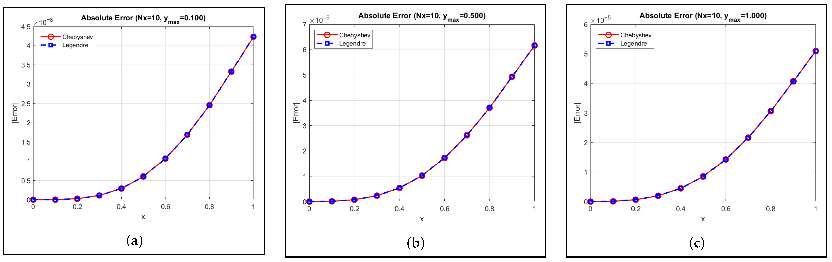
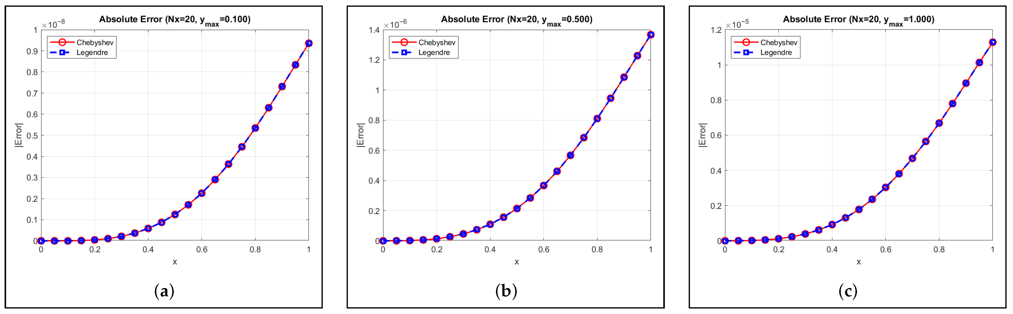
Case (1): For Equation (38) of linear type, the following is considered: h ( x , y ) = 1 , y [ 0 , 0.1 ] , λ 1 = λ 2 = 0.05 , τ 1 = τ 2 = 0.01 . The comparison of the error results obtained from the Chebyshev and Legendre polynomial methods are presented in Table 1, Table 2, Table 3, Table 4, Table 5 and Table 6. The absolute errors obtained from the Chebyshev and Legendre polynomial methods for Case (1) are illustrated in Figure 1 and Figure 2.
Case (2): For the second kind equation of nonlinear type, we consider
u ( x , y ) = g ( x , y )   +   0.05 0 1 e | x s | u ( s , y ) d s   +   0.05 0 y 0 1 e | x s | ( y   +   τ ) u s τ 1 , τ τ 2 2 d s d τ .
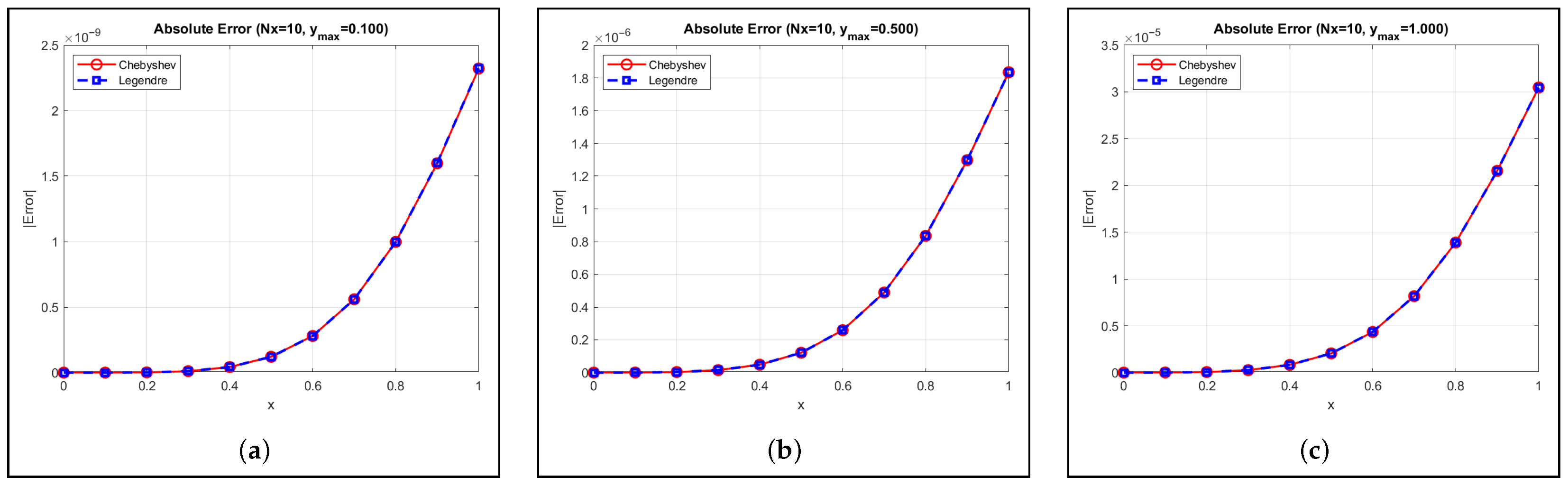
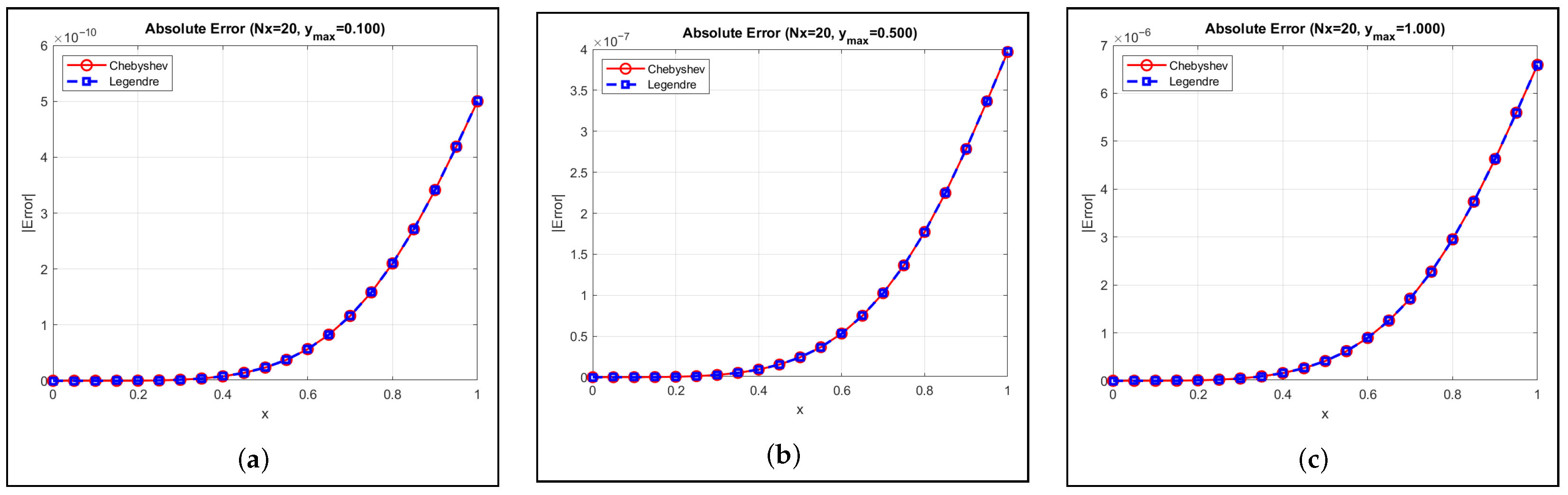
h ( x , y ) = 1 , y = 0.1 , 0.5 , 1 , λ 1 = λ 2 = 0.05 , a n d τ 1 = τ 2 = 0.01 . The comparison of the error results obtained from the Chebyshev and Legendre polynomial methods is presented in Table 7, Table 8, Table 9, Table 10, Table 11 and Table 12. The absolute errors obtained from the Chebyshev and Legendre polynomial methods for Case (2) are illustrated in Figure 3 and Figure 4.
Based on the previous application (38), the numerical results for both linear and nonlinear cases are analyzed and discussed below:
  • When applying the collocation method to linear functions utilizing Chebyshev and Legendre polynomials with N = 10 and N = 20 , the numerical error is very small at the beginning of the time domain, roughly 10 15 at x = 0 , and gradually increases with x. As shown in Table 1 and Table 4, the error remains limited during the initial interval. During the short time interval 0 y 0.1 , the error for both N values remains below 10 8 at x = 1 . As illustrated in Figure 1a and Figure 2a. Expanding the interval to 0 y 0.5 results in a larger error, reaching approximately 10 6 for N = 10 , whereas slightly lower values are observed for N = 20 as shown in Table 2 and Table 5, indicating improved accuracy with a larger number of polynomials. During the extended interval 0 y 1 , the error increases to approximately 10 5 for N = 10 , whereas it remains lower for N = 20 , demonstrating the effect of increasing N in reducing cumulative error. As shown in Figure 1c and Figure 2c.
    The results indicate that Chebyshev and Legendre polynomials exhibit comparable performance, with the error gradually increasing with x, without abrupt fluctuations, indicating the numerical stability of the collocation method for linear functions. Overall, longer time intervals lead to greater error accumulation, while increasing N reduces the error. The difference between Chebyshev and Legendre polynomials remains minimal in these linear cases.
  • In the nonlinear case, the numerical error is extremely small at the beginning of the time domain, about between 10 27 at x = 0 and 10 25 at x = 0 , respectively, and increases with x. As shown in Table 7 and Table 10. Over the short time interval 0 y 0.1 , the error remains very small for both N values, with a slight increase over this interval. Moreover, N = 20 consistently yields lower error, demonstrating the improved accuracy with an increased number of polynomials. Expanding the interval to 0 y 0.5 results in large error, ranging from 10 6 to 10 7 for N = 10 , while N = 20 maintains higher accuracy. During the extended interval 0 y 1 , the error significantly increases, ranging from 10 5 to 10 6 , whereas N = 20 continues to limit error accumulation.
The results indicate that Chebyshev and Legendre polynomials exhibit comparable performance, with the error gradually increasing with x and without abrupt fluctuations, indicating the numerical stability of the collocation method for nonlinear equations. Overall, increasing N enhances accuracy and reduces error, whereas longer time intervals lead to greater error accumulation. The difference between Chebyshev and Legendre polynomials remains a negligible effect even in these nonlinear cases.

5. Conclusions

This study introduces a novel and innovative approach to a comprehensive analytical and numerical investigation of DMIEs of the second kind, both linear and nonlinear, with continuous kernels, offering a thorough examination of the existence and convergence of solutions. The collocation method was employed to yield a dependable numerical approximation, utilizing Chebyshev and Legendre polynomials to represent the approximate solution, while the correctness of the suggested strategy was assessed by quantifying the resultant numerical errors.
The results reveal that the numerical approach attains a high degree of accuracy and exhibits steady convergence. The results demonstrate the efficacy of the numerical method used and the potential for its extension to encompass more categories of integral equations and more intricate computational applications.
The following provides a concise summary of the results obtained from the various applications:
(1)
As shown in Table 1, Table 2, Table 3, Table 4, Table 5, Table 6, Table 7, Table 8, Table 9, Table 10, Table 11 and Table 12, the Chebyshev and Legendre polynomial methods yield approximate solutions that closely match the exact values. The absolute errors are minimal, reaching as low as 10 27 in certain instances at the onset of the time domain, confirming the approach’s high precision and numerical stability.
(2)
Increasing the number of terms N markedly enhances accuracy and mitigates error buildup in both linear and nonlinear equations.
(3)
The duration of the time period inherently amplifies the buildup of numerical mistakes, becoming more evident over extended intervals such as y [ 0 , 1 ] .
(4)
Although numerical errors in nonlinear equations were slightly greater than in linear cases, the convergence and stability exhibited consistent behavior across both types.
(5)
The finding validates that the method applies to both linear and nonlinear equations with considerable efficiency.
The proposed numerical method demonstrates substantial reliability and adaptability, establishing a robust foundation for future investigations and enabling advancement toward more intricate or higher-dimensional classes of third-type DMIEs, among which are systems with variable or discontinuous kernels. The method’s capability to address complex problems or coupled integral differential equations can be systematically evaluated, thereby enhancing the understanding of their behavior in increasingly challenging scenarios.
The current findings highlight the effectiveness of the methodology in controlling error accumulation and achieving numerical convergence, underscoring the suitability of the approach for practical applications requiring high precision, such as those in engineering physics and biological modeling. Future extensions may also incorporate alternative polynomials, including Hermite, Lagrange, and Bernstein polynomials.

Author Contributions

A.M.A.-B.: Methodology, Supervision, Formal Analysis; R.S.A.-H.: Writing—Original Draft; A.M.S.M.: Writing—Review, Supervision. All authors have read and agreed to the published version of the manuscript.

Funding

This research received no external funding.

Data Availability Statement

This investigation was not supported by any data.

Conflicts of Interest

The authors declare no conflicts of interest.

References

  1. Kanwal, R.P. Linear Integral Equations; Springer Science & Business Media: Berlin/Heidelberg, Germany, 2013. [Google Scholar]
  2. Jerri, A.J. Introduction to Integral Equations with Applications; John Wiley & Sons: Hoboken, NJ, USA, 1999. [Google Scholar]
  3. Krasnov, M.L.; Kiselev, A.; Makarenko, G.I.; Yankovsky, G. Problems and Exercises in Integral Equations; MIR Publishers: Moscow, Russia, 1971. [Google Scholar]
  4. Delves, L.M.; Walsh, J. Numerical Solution of Integral Equations; Oxford University Press: Oxford, UK, 1974. [Google Scholar]
  5. Al-Bugami, A. Numerical Treatments of Functional Fredholm Integral Equation in 2D with Discontinuous Kernels. J. Appl. Math. Phys. 2023, 11, 3702–3711. [Google Scholar] [CrossRef]
  6. Al-Bugami, A. Numerical Treating of Mixed Integral Equation Two-Dimensional in Surface Cracks in Finite Layers of Materials. Adv. Math. Phys. 2022, 2022, 3398175. [Google Scholar] [CrossRef]
  7. Jan, A. Solution of nonlinear mixed integral equation via collocation method basing on orthogonal polynomials. Heliyon 2022, 8, e11827. [Google Scholar] [CrossRef] [PubMed]
  8. Jan, A. Numerical solution via a singular mixed integral equation in (2+1) dimensional. Appl. Math. Inf. Sci. 2022, 16, 871–882. [Google Scholar]
  9. Al-Bugami, A. Numerical solutions for nonlinear mixed integro-differential equation and the neutron transport equation. AIP Adv. 2024, 14, 045333. [Google Scholar] [CrossRef]
  10. Albugami, A. Adomian Decomposition Method and Block by Block Method for Solving Nonlinear Functional Volterra Integral Equation in Two-Dimensions. Eur. J. Pure Appl. Math. 2024, 17, 1070–1081. [Google Scholar] [CrossRef]
  11. Al-Bugami, A.; Abdou, M.A.; Mahdy, A. Sixth-kind Chebyshev and Bernoulli polynomial numerical methods for solving nonlinear mixed partial integrodifferential equations with continuous kernels. J. Funct. Spaces 2023, 2023, 6647649. [Google Scholar] [CrossRef]
  12. Al-Bugami, A. Efficient Numerical Algorithm for the Solution of Nonlinear Two-Dimensional Volterra Integral Equation Arising from Torsion Problem. Adv. Math. Phys. 2021, 2021, 6559694. [Google Scholar] [CrossRef]
  13. Mahdy, A.; Abdou, M.; Mohamed, D.S. Numerical solution and dynamical studies for (2+1) dimensional Volterra–Fredholm integral equations with a discontinuous kernel. J. Appl. Math. Comput. 2025, 71, 3671–3697. [Google Scholar] [CrossRef]
  14. Yatsenko, Y. Volterra integral equations with unknown delay time. Methods Appl. Anal. 1995, 2, 408–419. [Google Scholar] [CrossRef]
  15. Muhammad, A.M.; Ayal, A. Numerical solution of linear Volterra integral equation with delay using Bernstein polynomial. Int. Electron. J. Math. Educ. 2019, 14, 735–740. [Google Scholar] [CrossRef] [PubMed]
  16. Cimen, E.; Yatar, S. Numerical solution of Volterra integro-differential equation with delay. J. Math. Comput. Sci. 2020, 20, 255–263. [Google Scholar] [CrossRef]
  17. Al-Jubory, A.K.O. Approximate Solution of Delay Integral Equations via Functions of two Variable. J. Phys. Conf. Ser. 2021, 1879, 022127. [Google Scholar] [CrossRef]
  18. Raad, S.A.; Abdou, M.A. The Effect of Fractional Order of Time Phase Delay via a Mixed Integral Equation in (2+1) Dimensions with an Extended Discontinuous Kernel. Symmetry 2025, 17, 36. [Google Scholar] [CrossRef]
  19. Shen, J.; Tang, T. Spectral and High-Order Methods with Applications; Science Press: Beijing, China, 2006. [Google Scholar]
  20. Canuto, C.; Hussaini, M.Y.; Quarteroni, A.; Zang, T.A. Spectral Methods: Fundamentals in Single Domains; Springer: Berlin/Heidelberg, Germany, 2010. [Google Scholar]
Figure 1. Absolute errors of the Chebyshev and Legendre polynomials methods applied to the linear second kind equation for N = 10 . (a) y [ 0 , 0.1 ] ; (b) y [ 0 , 0.5 ] ; (c) y [ 0 , 1 ] .
Mca 31 00059 g001
Figure 2. Absolute errors of the Chebyshev and Legendre polynomials methods applied to the linear second kind equation for N = 20 . (a) y [ 0 , 0.1 ] ; (b) y [ 0 , 0.5 ] ; (c) y [ 0 , 1 ] .
Mca 31 00059 g002
Figure 3. Absolute errors of the Chebyshev and Legendre polynomials methods applied to the nonlinear second kind equation for N = 10 . (a) y [ 0 , 0.1 ] ; (b) y [ 0 , 0.5 ] ; (c) y [ 0 , 1 ] .
Mca 31 00059 g003
Figure 4. Absolute errors of the Chebyshev and Legendre polynomials methods applied to the nonlinear second kind equation for N = 20 . (a) y [ 0 , 0.1 ] ; (b) y [ 0 , 0.5 ] ; (c) y [ 0 , 1 ] .
Mca 31 00059 g004
Table 1. The exact, numerical and the absolute error results of the collocation method in Chebyshev and Legendre polynomials methods at h ( x , y ) = 1 , y [ 0 , 0.1 ] , N = 10 .
xExact SolutionChebyshev PolynomialsError of ChebyshevLegendre PolynomialsError of Legendre
0.0000.000000000000000   ×   10 0 −2.3692796162   ×   10 15 2.3692796162   ×   10 15 −2.4400900190   ×   10 15 2.4400900190   ×   10 15
0.1001.000000000000000   ×   10 4 9.9999999994   ×   10 5 5.6593456050   ×   10 15 9.9999999941   ×   10 5 5.9196218890   ×   10 15
0.2008.000000000000001   ×   10 4 8.0000024827   ×   10 4 2.4827497729   ×   10 10 8.0000024803   ×   10 4 2.4803408838   ×   10 10
0.3002.700000000000001   ×   10 3 2.7000010979   ×   10 3 1.0979156767   ×   10 9 2.7000010980   ×   10 3 1.0980369348   ×   10 9
0.4006.400000000000001   ×   10 3 6.4000029145   ×   10 3 2.9145077280   ×   10 9 6.4000029134   ×   10 3 2.9134748016   ×   10 9
0.5001.250000000000000   ×   10 2 1.2500006025   ×   10 2 6.0258168264   ×   10 9 1.2500006019   ×   10 2 6.0193175582   ×   10 9
0.6002.160000000000001   ×   10 2 2.1600010643   ×   10 2 1.0643498311   ×   10 8 2.1600010639   ×   10 2 1.0639599298   ×   10 8
0.7003.430000000000001   ×   10 2 3.4300016850   ×   10 2 1.6850813827   ×   10 8 3.4300016852   ×   10 2 1.6852343888   ×   10 8
0.8005.120000000000001   ×   10 2 5.1200024565   ×   10 2 2.4565013134   ×   10 8 5.1200024541   ×   10 2 2.4541108999   ×   10 8
0.9007.290000000000001   ×   10 2 7.2900033227   ×   10 2 3.3227565046   ×   10 8 7.2900033261   ×   10 2 3.3261942603   ×   10 8
1.0001.000000000000000   ×   10 1 1.0000004231   ×   10 1 4.2317127441   ×   10 8 1.0000004235   ×   10 1 4.2350381521   ×   10 8
Table 2. The exact, numerical and the absolute error results of the collocation method in Chebyshev and Legendre polynomials methods at h ( x , y ) = 1 , y [ 0 , 0.5 ] , N = 10 .
xExact SolutionChebyshev PolynomialsError of ChebyshevLegendre PolynomialsError of Legendre
0.0000.000000000000000   ×   10 0 −4.9760583987   ×   10 16 4.9760583987   ×   10 16 −1.0635264356   ×   10 16 1.0635264356   ×   10 16
0.1005.000000000000001   ×   10 4 5.0001165887   ×   10 4 1.1658872621   ×   10 8 5.0001165888   ×   10 4 1.1658884075   ×   10 8
0.2004.000000000000001   ×   10 3 4.0000744988   ×   10 3 7.4498860709   ×   10 8 4.0000744988   ×   10 3 7.4498834237   ×   10 8
0.3001.350000000000001   ×   10 2 1.3500234613   ×   10 2 2.3461380789   ×   10 7 1.3500234613   ×   10 2 2.3461379275   ×   10 7
0.4003.200000000000001   ×   10 2 3.2000537607   ×   10 2 5.3760769604   ×   10 7 3.2000537607   ×   10 2 5.3760761031   ×   10 7
0.5006.250000000000000   ×   10 2 6.2501022618   ×   10 2 1.0226183255   ×   10 6 6.2501022617   ×   10 2 1.0226179313   ×   10 6
0.6001.080000000000000   ×   10 1 1.0800171472   ×   10 1 1.7147230383   ×   10 6 1.0800171472   ×   10 1 1.7147227179   ×   10 6
0.7001.715000000000000   ×   10 1 1.7150261795   ×   10 1 2.6179504257   ×   10 6 1.7150261795   ×   10 1 2.6179502289   ×   10 6
0.8002.560000000000001   ×   10 1 2.5600370878   ×   10 1 3.7087833488   ×   10 6 2.5600370878   ×   10 1 3.7087821432   ×   10 6
0.9003.645000000000000   ×   10 1 3.6450492568   ×   10 1 4.9256896723   ×   10 6 3.6450492569   ×   10 1 4.9256934289   ×   10 6
1.0005.000000000000000   ×   10 1 5.0000616639   ×   10 1 6.1663972200   ×   10 6 5.0000616639   ×   10 1 6.1663998213   ×   10 6
Table 3. The exact, numerical and the absolute error results of the collocation method in Chebyshev and Legendre polynomials methods at h ( x , y ) = 1 , y [ 0 , 1 ] , N = 10 .
xExact SolutionChebyshev PolynomialsError of ChebyshevLegendre PolynomialsError of Legendre
0.0000.000000000000000   ×   10 0 −8.4790690855   ×   10 15 8.4790690855   ×   10 15 −1.9109081733   ×   10 15 1.9109081733   ×   10 15
0.1001.000000000000000   ×   10 3 1.0001049851   ×   10 3 1.0498514609   ×   10 7 1.0001049853   ×   10 3 1.0498530368   ×   10 7
0.2008.000000000000002   ×   10 3 8.0006402266   ×   10 3 6.4022664735   ×   10 7 8.0006402264   ×   10 3 6.4022640789   ×   10 7
0.3002.700000000000001   ×   10 2 2.7001978266   ×   10 2 1.9782661981   ×   10 6 2.7001978266   ×   10 2 1.9782660569   ×   10 6
0.4006.400000000000002   ×   10 2 6.4004488528   ×   10 2 4.4885281477   ×   10 6 6.4004488527   ×   10 2 4.4885273858   ×   10 6
0.5001.250000000000000   ×   10 1 1.2500849009   ×   10 1 8.4900971424   ×   10 6 1.2500849009   ×   10 1 8.4900937887   ×   10 6
0.6002.160000000000001   ×   10 1 2.1601419063   ×   10 1 1.4190633954   ×   10 5 2.1601419063   ×   10 1 1.4190631253   ×   10 5
0.7003.430000000000000   ×   10 1 3.4302162964   ×   10 1 2.1629643561   ×   10 5 3.4302162964   ×   10 1 2.1629641924   ×   10 5
0.8005.120000000000001   ×   10 1 5.1203062455   ×   10 1 3.0624558938   ×   10 5 5.1203062454   ×   10 1 3.0624548916   ×   10 5
0.9007.290000000000001   ×   10 1 7.2904068291   ×   10 1 4.0682917737   ×   10 5 7.2904068294   ×   10 1 4.0682948923   ×   10 5
1.0001.000000000000000   ×   10 0 1.0000509768   ×   10 0 5.0976851816   ×   10 5 1.0000509768   ×   10 0 5.0976873446   ×   10 5
Table 4. The Description of the exact, numerical and the absolute error results of the collocation method in Chebyshev and Legendre polynomials methods at h ( x , y ) = 1 , y [ 0 , 0.1 ] , N = 20 .
xExact SolutionChebyshev PolynomialsError of ChebyshevLegendre PolynomialsError of Legendre
0.0000.000000000000000   ×   10 0 −2.2270981876   ×   10 16 2.2270981876   ×   10 16 −2.2824141958   ×   10 16 2.2824141958   ×   10 16
0.0501.250000000000000   ×   10 5 1.2499999999   ×   10 5 4.9526016425   ×   10 16 1.2499999999   ×   10 5 5.0673915476   ×   10 16
0.1001.000000000000000   ×   10 4 9.9999999999   ×   10 5 5.5973292407   ×   10 16 9.9999999999   ×   10 5 5.7946540361   ×   10 16
0.1503.375000000000001   ×   10 4 3.3750001065   ×   10 4 1.0659532230   ×   10 11 3.3750001065   ×   10 4 1.0658744937   ×   10 11
0.2008.000000000000001   ×   10 4 8.0000004197   ×   10 4 4.1978533496   ×   10 11 8.0000004197   ×   10 4 4.1971808190   ×   10 11
0.2501.562500000000000   ×   10 3 1.5625001044   ×   10 3 1.0441603419   ×   10 10 1.5625001043   ×   10 3 1.0439993270   ×   10 10
0.3002.700000000000001   ×   10 3 2.7000002086   ×   10 3 2.0860754660   ×   10 10 2.7000002085   ×   10 3 2.0857726570   ×   10 10
0.3504.287500000000001   ×   10 3 4.2875003651   ×   10 3 3.6516137683   ×   10 10 4.2875003650   ×   10 3 3.6509748176   ×   10 10
0.4006.400000000000001   ×   10 3 6.4000005843   ×   10 3 5.8439437230   ×   10 10 6.4000005842   ×   10 3 5.8425553804   ×   10 10
0.4509.112500000000001   ×   10 3 9.1125008759   ×   10 3 8.7591618333   ×   10 10 9.1125008756   ×   10 3 8.7565325476   ×   10 10
0.5001.250000000000000   ×   10 2 1.2500001248   ×   10 2 1.2480650037   ×   10 9 1.2500001247   ×   10 2 1.2476537563   ×   10 9
0.5501.663750000000001   ×   10 2 1.6637501707   ×   10 2 1.7072802165   ×   10 9 1.6637501706   ×   10 2 1.7067490754   ×   10 9
0.6002.160000000000001   ×   10 2 2.1600002257   ×   10 2 2.2575359880   ×   10 9 2.1600002256   ×   10 2 2.2569570344   ×   10 9
0.6502.746250000000000   ×   10 2 2.7462502899   ×   10 2 2.8999395593   ×   10 9 2.7462502899   ×   10 2 2.8993700808   ×   10 9
0.7003.430000000000001   ×   10 2 3.4300003632   ×   10 2 3.6325207009   ×   10 9 3.4300003631   ×   10 2 3.6319303953   ×   10 9
0.7504.218750000000000   ×   10 2 4.2187504450   ×   10 2 4.4501280022   ×   10 9 4.2187504449   ×   10 2 4.4494052470   ×   10 9
0.8005.120000000000001   ×   10 2 5.1200005344   ×   10 2 5.3442398770   ×   10 9 5.1200005343   ×   10 2 5.3433947891   ×   10 9
0.8506.141250000000002   ×   10 2 6.1412506302   ×   10 2 6.3024526639   ×   10 9 6.1412506302   ×   10 2 6.3020454965   ×   10 9
0.9007.290000000000001   ×   10 2 7.2900007307   ×   10 2 7.3075005907   ×   10 9 7.2900007308   ×   10 2 7.3089974073   ×   10 9
0.9508.573750000000001   ×   10 2 8.5737508335   ×   10 2 8.3359853464   ×   10 9 8.5737508341   ×   10 2 8.3410068990   ×   10 9
1.0001.000000000000000   ×   10 1 1.0000000935   ×   10 1 9.3576590087   ×   10 9 1.0000000936   ×   10 1 9.3637108067   ×   10 9
Table 5. The exact, numerical and the absolute error results of the collocation method in Chebyshev and Legendre polynomials methods at h ( x , y ) = 1 , y [ 0 , 0.5 ] , N = 20 .
xExact SolutionChebyshev PolynomialsError of ChebyshevLegendre PolynomialsError of Legendre
0.0000.000000000000000   ×   10 0 −9.3757685186   ×   10 16 9.3757685186   ×   10 16 −8.8758613378   ×   10 16 8.8758613378   ×   10 16
0.0506.250000000000001   ×   10 5 6.2500247584   ×   10 5 2.4758400337   ×   10 10 6.2500247584   ×   10 5 2.4758412155   ×   10 10
0.1005.000000000000001   ×   10 4 5.0000176200   ×   10 4 1.7620001452   ×   10 9 5.0000176200   ×   10 4 1.7620002882   ×   10 9
0.1501.687500000000001   ×   10 3 1.6875057772   ×   10 3 5.7772671720   ×   10 9 1.6875057772   ×   10 3 5.7772671238   ×   10 9
0.2004.000000000000001   ×   10 3 4.0000136054   ×   10 3 1.3605402655   ×   10 8 4.0000136054   ×   10 3 1.3605402151   ×   10 8
0.2507.812500000000000   ×   10 3 7.8125265898   ×   10 3 2.6589856341   ×   10 8 7.8125265898   ×   10 3 2.6589855425   ×   10 8
0.3001.350000000000001   ×   10 2 1.3500046077   ×   10 2 4.6077877026   ×   10 8 1.3500046077   ×   10 2 4.6077875785   ×   10 8
0.3502.143750000000001   ×   10 2 2.1437573397   ×   10 2 7.3397561556   ×   10 8 2.1437573397   ×   10 2 7.3397559294   ×   10 8
0.4003.200000000000001   ×   10 2 3.2000109823   ×   10 2 1.0982304462   ×   10 7 3.2000109823   ×   10 2 1.0982303980   ×   10 7
0.4504.556250000000001   ×   10 2 4.5562656518   ×   10 2 1.5651818651   ×   10 7 4.5562656518   ×   10 2 1.5651817723   ×   10 7
0.5006.250000000000000   ×   10 2 6.2500214459   ×   10 2 2.1445975824   ×   10 7 6.2500214459   ×   10 2 2.1445974361   ×   10 7
0.5508.318750000000003   ×   10 2 8.3187784351   ×   10 2 2.8435114982   ×   10 7 8.3187784351   ×   10 2 2.8435113091   ×   10 7
0.6001.080000000000000   ×   10 1 1.0800036654   ×   10 1 3.6654373024   ×   10 7 1.0800036654   ×   10 1 3.6654370982   ×   10 7
0.6501.373125000000000   ×   10 1 1.3731296098   ×   10 1 4.6098294204   ×   10 7 1.3731296098   ×   10 1 4.6098292236   ×   10 7
0.7001.715000000000000   ×   10 1 1.7150056718   ×   10 1 5.6718885496   ×   10 7 1.7150056718   ×   10 1 5.6718883528   ×   10 7
0.7502.109375000000000   ×   10 1 2.1093818426   ×   10 1 6.8426614263   ×   10 7 2.1093818426   ×   10 1 6.8426612015   ×   10 7
0.8002.560000000000001   ×   10 1 2.5600081091   ×   10 1 8.1091726272   ×   10 7 2.5600081091   ×   10 1 8.1091723946   ×   10 7
0.8503.070625000000001   ×   10 1 3.0706344540   ×   10 1 9.4540706024   ×   10 7 3.0706344540   ×   10 1 9.4540705758   ×   10 7
0.9003.645000000000000   ×   10 1 3.6450108540   ×   10 1 1.0854002014   ×   10 6 3.6450108540   ×   10 1 1.0854002702   ×   10 6
0.9504.286875000000000   ×   10 1 4.2868872756   ×   10 1 1.2275689768   ×   10 6 4.2868872756   ×   10 1 1.2275691610   ×   10 6
1.0005.000000000000000   ×   10 1 5.0000136685   ×   10 1 1.3668533260   ×   10 6 5.0000136685   ×   10 1 1.3668534957   ×   10 6
Table 6. The exact, numerical and the absolute error results of the collocation method in Chebyshev and Legendre polynomials methods at h ( x , y ) = 1 , y [ 0 , 1 ] , N = 20 .
xExact SolutionChebyshev PolynomialsError of ChebyshevLegendre PolynomialsError of Legendre
0.0000.000000000000000   ×   10 0 −1.5353814748   ×   10 14 1.5353814748   ×   10 14 −1.4514359599   ×   10 14 1.4514359599   ×   10 14
0.0501.250000000000000   ×   10 4 1.2500264131   ×   10 4 2.6413187601   ×   10 9 1.2500264132   ×   10 4 2.6413215641   ×   10 9
0.1001.000000000000000   ×   10 3 1.0000165073   ×   10 3 1.6507318579   ×   10 8 1.0000165073   ×   10 3 1.6507320382   ×   10 8
0.1503.375000000000001   ×   10 3 3.3750515770   ×   10 3 5.1577072631   ×   10 8 3.3750515770   ×   10 3 5.1577071663   ×   10 8
0.2008.000000000000002   ×   10 3 8.0001184338   ×   10 3 1.1843385696   ×   10 7 8.0001184338   ×   10 3 1.1843385157   ×   10 7
0.2501.562500000000000   ×   10 2 1.5625227909   ×   10 2 2.2790910617   ×   10 7 1.5625227909   ×   10 2 2.2790909686   ×   10 7
0.3002.700000000000001   ×   10 2 2.7000390877   ×   10 2 3.9087765102   ×   10 7 2.7000390877   ×   10 2 3.9087763795   ×   10 7
0.3504.287500000000001   ×   10 2 4.2875618083   ×   10 2 6.1808386307   ×   10 7 4.2875618083   ×   10 2 6.1808384087   ×   10 7
0.4006.400000000000002   ×   10 2 6.4000919864   ×   10 2 9.1986488647   ×   10 7 6.4000919864   ×   10 2 9.1986484208   ×   10 7
0.4509.112500000000001   ×   10 2 9.1126305695   ×   10 2 1.3056952730   ×   10 6 9.1126305695   ×   10 2 1.3056951911   ×   10 6
0.5001.250000000000000   ×   10 1 1.2500178356   ×   10 1 1.7835639002   ×   10 6 1.2500178356   ×   10 1 1.7835637739   ×   10 6
0.5501.663750000000001   ×   10 1 1.6637735927   ×   10 1 2.3592743881   ×   10 6 1.6637735927   ×   10 1 2.3592742269   ×   10 6
0.6002.160000000000001   ×   10 1 2.1600303580   ×   10 1 3.0358082041   ×   10 6 2.1600303580   ×   10 1 3.0358080310   ×   10 6
0.6502.746250000000000   ×   10 1 2.7462881288   ×   10 1 3.8128877056   ×   10 6 2.7462881288   ×   10 1 3.8128875394   ×   10 6
0.7003.430000000000000   ×   10 1 3.4300468681   ×   10 1 4.6868154885   ×   10 6 3.4300468681   ×   10 1 4.6868153236   ×   10 6
0.7504.218750000000000   ×   10 1 4.2188065054   ×   10 1 5.6505461346   ×   10 6 4.2188065054   ×   10 1 5.6505459460   ×   10 6
0.8005.120000000000001   ×   10 1 5.1200669377   ×   10 1 6.6937749045   ×   10 6 5.1200669377   ×   10 1 6.6937747098   ×   10 6
0.8506.141250000000001   ×   10 1 6.1413280262   ×   10 1 7.8026218008   ×   10 6 6.1413280262   ×   10 1 7.8026217787   ×   10 6
0.9007.290000000000001   ×   10 1 7.2900895827   ×   10 1 8.9582740572   ×   10 6 7.2900895827   ×   10 1 8.9582746265   ×   10 6
0.9508.573750000000000   ×   10 1 8.5738513375   ×   10 1 1.0133759432   ×   10 5 8.5738513376   ×   10 1 1.0133760959   ×   10 5
1.0001.000000000000000   ×   10 0 1.0000112878   ×   10 0 1.1287899312   ×   10 5 1.0000112879   ×   10 0 1.1287900718   ×   10 5
Table 7. The exact, numerical, and absolute error results for Case (2) by using the collocation method in Chebyshev and Legendre polynomial methods at h ( x , y ) = 1 , y [ 0 , 0.1 ] , N = 10 .
xExact SolutionChebyshev PolynomialsError of ChebyshevLegendre PolynomialsError of Legendre
0.0000.000000000000000   ×   10 0 −1.8949123403   ×   10 24 1.8949123403   ×   10 24 2.8827153243   ×   10 27 2.8827153243   ×   10 27
0.1001.000000000000000   ×   10 4 9.9999999999   ×   10 5 2.9951085014   ×   10 18 1.0000000000   ×   10 4 1.9380113833   ×   10 18
0.2008.000000000000001   ×   10 4 8.0000000133   ×   10 4 1.3336249422   ×   10 12 8.0000000133   ×   10 4 1.3327793729   ×   10 12
0.3002.700000000000001   ×   10 3 2.7000000105   ×   10 3 1.0593920705   ×   10 11 2.7000000105   ×   10 3 1.0599486999   ×   10 11
0.4006.400000000000001   ×   10 3 6.4000000422   ×   10 3 4.2272162333   ×   10 11 6.4000000422   ×   10 3 4.2262440942   ×   10 11
0.5001.250000000000000   ×   10 2 1.2500000120   ×   10 2 1.2067849670   ×   10 10 1.2500000120   ×   10 2 1.2055603564   ×   10 10
0.6002.160000000000001   ×   10 2 2.1600000279   ×   10 2 2.7956000014   ×   10 10 2.1600000279   ×   10 2 2.7945535815   ×   10 10
0.7003.430000000000001   ×   10 2 3.4300000559   ×   10 2 5.5939952670   ×   10 10 3.4300000559   ×   10 2 5.5928577047   ×   10 10
0.8005.120000000000001   ×   10 2 5.1200000997   ×   10 2 9.9761249955   ×   10 10 5.1200000996   ×   10 2 9.9637784134   ×   10 10
0.9007.290000000000001   ×   10 2 7.2900001597   ×   10 2 1.5976584083   ×   10 9 7.2900001598   ×   10 2 1.5989380930   ×   10 9
1.0001.000000000000000   ×   10 1 1.0000000232   ×   10 1 2.3211255972   ×   10 9 1.0000000232   ×   10 1 2.3232223922   ×   10 9
Table 8. The exact, numerical and the absolute error results for Case (2) by using the collocation method in Chebyshev and Legendre polynomials methods at h ( x , y ) = 1 , y [ 0 , 0.5 ] , N = 10 .
xExact SolutionChebyshev PolynomialsError of ChebyshevLegendre PolynomialsError of Legendre
0.0000.000000000000000   ×   10 0 1.6308395435   ×   10 18 1.6308395435   ×   10 18 3.2467781608   ×   10 19 3.2467781608   ×   10 19
0.1005.000000000000001   ×   10 4 5.0000024185   ×   10 4 2.4185125820   ×   10 10 5.0000024185   ×   10 4 2.4185147341   ×   10 10
0.2004.000000000000001   ×   10 3 4.0000030997   ×   10 3 3.0997640348   ×   10 9 4.0000030997   ×   10 3 3.0997638188   ×   10 9
0.3001.350000000000001   ×   10 2 1.3500015047   ×   10 2 1.5047730698   ×   10 8 1.3500015047   ×   10 2 1.5047731241   ×   10 8
0.4003.200000000000001   ×   10 2 3.2000048157   ×   10 2 4.8157080725   ×   10 8 3.2000048157   ×   10 2 4.8157081704   ×   10 8
0.5006.250000000000000   ×   10 2 6.2500121137   ×   10 2 1.2113768223   ×   10 7 6.2500121137   ×   10 2 1.2113765776   ×   10 7
0.6001.080000000000000   ×   10 1 1.0800025889   ×   10 1 2.5889555055   ×   10 7 1.0800025889   ×   10 1 2.5889546662   ×   10 7
0.7001.715000000000000   ×   10 1 1.7150048926   ×   10 1 4.8926168869   ×   10 7 1.7150048926   ×   10 1 4.8926151627   ×   10 7
0.8002.560000000000001   ×   10 1 2.5600083484   ×   10 1 8.3484237722   ×   10 7 2.5600083484   ×   10 1 8.3484217316   ×   10 7
0.9003.645000000000000   ×   10 1 3.6450129720   ×   10 1 1.2972044038   ×   10 6 3.6450129720   ×   10 1 1.2972050223   ×   10 6
1.0005.000000000000000   ×   10 1 5.0000183408   ×   10 1 1.8340858319   ×   10 6 5.0000183408   ×   10 1 1.8340867210   ×   10 6
Table 9. The exact, numerical and the absolute error results for Case (2) by using the collocation method in Chebyshev and Legendre polynomials methods at h ( x , y ) = 1 , y [ 0 , 1 ] , N = 10 .
xExact SolutionChebyshev PolynomialsError of ChebyshevLegendre PolynomialsError of Legendre
0.0000.000000000000000   ×   10 0 1.2347357694   ×   10 16 1.2347357694   ×   10 16 2.4596155833   ×   10 17 2.4596155833   ×   10 17
0.1001.000000000000000   ×   10 3 1.0000048976   ×   10 3 4.8976851500   ×   10 9 1.0000048976   ×   10 3 4.8976896858   ×   10 9
0.2008.000000000000002   ×   10 3 8.0000562388   ×   10 3 5.6238865349   ×   10 8 8.0000562388   ×   10 3 5.6238867405   ×   10 8
0.3002.700000000000001   ×   10 2 2.7000262651   ×   10 2 2.6265112192   ×   10 7 2.7000262651   ×   10 2 2.6265114102   ×   10 7
0.4006.400000000000002   ×   10 2 6.4000824013   ×   10 2 8.2401370787   ×   10 7 6.4000824013   ×   10 2 8.2401373112   ×   10 7
0.5001.250000000000000   ×   10 1 1.2500204831   ×   10 1 2.0483148952   ×   10 6 1.2500204831   ×   10 1 2.0483144849   ×   10 6
0.6002.160000000000001   ×   10 1 2.1600434457   ×   10 1 4.3445780929   ×   10 6 2.1600434457   ×   10 1 4.3445766831   ×   10 6
0.7003.430000000000000   ×   10 1 3.4300817012   ×   10 1 8.1701200863   ×   10 6 3.4300817011   ×   10 1 8.1701171814   ×   10 6
0.8005.120000000000001   ×   10 1 5.1201389829   ×   10 1 1.3898298531   ×   10 5 5.1201389829   ×   10 1 1.3898295066   ×   10 5
0.9007.290000000000001   ×   10 1 7.2902155987   ×   10 1 2.1559872973   ×   10 5 7.2902155988   ×   10 1 2.1559883271   ×   10 5
1.0001.000000000000000   ×   10 0 1.0000304670   ×   10 0 3.0467074954   ×   10 5 1.0000304670   ×   10 0 3.0467089818   ×   10 5
Table 10. The exact, numerical and the absolute error results for Case (2) by using the collocation method in Chebyshev and Legendre polynomials methods at h ( x , y ) = 1 , y [ 0 , 0.1 ] , N = 20 .
xExact SolutionChebyshev PolynomialsError of ChebyshevLegendre PolynomialsError of Legendre
0.0000.000000000000000   ×   10 0 −7.1456393935   ×   10 25 7.1456393935   ×   10 25 −2.0818124307   ×   10 25 2.0818124307   ×   10 25
0.0501.250000000000000   ×   10 5 1.2500000000   ×   10 5 2.2022856628   ×   10 20 1.2500000000   ×   10 5 2.4394548880   ×   10 18
0.1001.000000000000000   ×   10 4 1.0000000000   ×   10 4 1.4772254600   ×   10 18 1.0000000000   ×   10 4 3.9437854024   ×   10 18
0.1503.375000000000001   ×   10 4 3.3750000002   ×   10 4 2.7853424861   ×   10 14 3.3750000002   ×   10 4 2.7859604814   ×   10 14
0.2008.000000000000001   ×   10 4 8.0000000019   ×   10 4 1.9000859913   ×   10 13 8.0000000019   ×   10 4 1.9001597170   ×   10 13
0.2501.562500000000000   ×   10 3 1.5625000006   ×   10 3 6.8431718625   ×   10 13 1.5625000006   ×   10 3 6.8434580918   ×   10 13
0.3002.700000000000001   ×   10 3 2.7000000018   ×   10 3 1.8179841312   ×   10 12 2.7000000018   ×   10 3 1.8180301014   ×   10 12
0.3504.287500000000001   ×   10 3 4.2875000040   ×   10 3 4.0257554234   ×   10 12 4.2875000040   ×   10 3 4.0255680733   ×   10 12
0.4006.400000000000001   ×   10 3 6.4000000078   ×   10 3 7.8858898577   ×   10 12 6.4000000078   ×   10 3 7.8846894291   ×   10 12
0.4509.112500000000001   ×   10 3 9.1125000141   ×   10 3 1.4129974967   ×   10 11 9.1125000141   ×   10 3 1.4126484704   ×   10 11
0.5001.250000000000000   ×   10 2 1.2500000023   ×   10 2 2.3642225330   ×   10 11 1.2500000023   ×   10 2 2.3635121637   ×   10 11
0.5501.663750000000001   ×   10 2 1.6637500037   ×   10 2 3.7443957656   ×   10 11 1.6637500037   ×   10 2 3.7432466848   ×   10 11
0.6002.160000000000001   ×   10 2 2.1600000056   ×   10 2 5.6659621439   ×   10 11 2.1600000056   ×   10 2 5.6643481571   ×   10 11
0.6502.746250000000000   ×   10 2 2.7462500082   ×   10 2 8.2461003303   ×   10 11 2.7462500082   ×   10 2 8.2438982723   ×   10 11
0.7003.430000000000001   ×   10 2 3.4300000115   ×   10 2 1.1598527693   ×   10 10 3.4300000115   ×   10 2 1.1595310822   ×   10 10
0.7504.218750000000000   ×   10 2 4.2187500158   ×   10 2 1.5822095716   ×   10 10 4.2187500158   ×   10 2 1.5817196857   ×   10 10
0.8005.120000000000001   ×   10 2 5.1200000209   ×   10 2 2.0985285731   ×   10 10 5.1200000209   ×   10 2 2.0978679904   ×   10 10
0.8506.141250000000002   ×   10 2 6.1412500271   ×   10 2 2.7105447053   ×   10 10 6.1412500270   ×   10 2 2.7099863325   ×   10 10
0.9007.290000000000001   ×   10 2 7.2900000341   ×   10 2 3.4121534764   ×   10 10 7.2900000341   ×   10 2 3.4124827963   ×   10 10
0.9508.573750000000001   ×   10 2 8.5737500418   ×   10 2 4.1859642141   ×   10 10 8.5737500418   ×   10 2 4.1882884660   ×   10 10
1.0001.000000000000000   ×   10 1 1.0000000049   ×   10 1 4.9991992490   ×   10 10 1.0000000050   ×   10 1 5.0030658782   ×   10 10
Table 11. The exact, numerical and the absolute error results for Case (2) by using the collocation method in Chebyshev and Legendre polynomials methods at h ( x , y ) = 1 , y [ 0 , 0.5 ] , N = 20 .
xExact SolutionChebyshev PolynomialsError of ChebyshevLegendre PolynomialsError of Legendre
0.0000.000000000000000   ×   10 0 −3.2381097566   ×   10 17 3.2381097566   ×   10 17 −3.5134233301   ×   10 17 3.5134233301   ×   10 17
0.0506.2500000000   ×   10 5 6.2500001890   ×   10 5 1.8904229716   ×   10 12 6.2500001891   ×   10 5 1.8915335064   ×   10 12
0.1005.0000000000   ×   10 4 5.0000003126   ×   10 4 3.1262410737   ×   10 11 5.0000003127   ×   10 4 3.1271440189   ×   10 11
0.1501.6875000000   ×   10 3 1.6875001590   ×   10 3 1.5901094178   ×   10 10 1.6875001590   ×   10 3 1.5902401379   ×   10 10
0.2004.0000000000   ×   10 3 4.0000005120   ×   10 3 5.1205213767   ×   10 10 4.0000005120   ×   10 3 5.1206934959   ×   10 10
0.2507.8125000000   ×   10 3 7.8125012843   ×   10 3 1.2843887359   ×   10 9 7.8125012844   ×   10 3 1.2844448872   ×   10 9
0.3001.3500000000   ×   10 2 1.3500002748   ×   10 2 2.7488432068   ×   10 9 1.3500002748   ×   10 2 2.7489129410   ×   10 9
0.3502.1437500000   ×   10 2 2.1437505268   ×   10 2 5.2684046743   ×   10 9 2.1437505268   ×   10 2 5.2681525461   ×   10 9
0.4003.2000000000   ×   10 2 3.2000009304   ×   10 2 9.3049834296   ×   10 9 3.2000009303   ×   10 2 9.3035618237   ×   10 9
0.4504.5562500000   ×   10 2 4.5562515422   ×   10 2 1.5422690187   ×   10 8 4.5562515418   ×   10 2 1.5418870555   ×   10 8
0.5006.2500000000   ×   10 2 6.2500024282   ×   10 2 2.4282709482   ×   10 8 6.2500024275   ×   10 2 2.4275400786   ×   10 8
0.5508.3187500000   ×   10 2 8.3187536627   ×   10 2 3.6627222088   ×   10 8 8.3187536615   ×   10 2 3.6615982648   ×   10 8
0.6001.0800000000   ×   10 1 1.0800005325   ×   10 1 5.3250263434   ×   10 8 1.0800005323   ×   10 1 5.3235090308   ×   10 8
0.6501.3731250000   ×   10 1 1.3731257495   ×   10 1 7.4953442702   ×   10 8 1.3731257493   ×   10 1 7.4933409172   ×   10 8
0.7001.7150000000   ×   10 1 1.7150010248   ×   10 1 1.0248374890   ×   10 7 1.7150010245   ×   10 1 1.0245529791   ×   10 7
0.7502.1093750000   ×   10 1 2.1093763644   ×   10 1 1.3644913166   ×   10 7 2.1093763640   ×   10 1 1.3640684262   ×   10 7
0.8002.5600000000   ×   10 1 2.5600017720   ×   10 1 1.7720545897   ×   10 7 2.5600017714   ×   10 1 1.7714965161   ×   10 7
0.8503.0706250000   ×   10 1 3.0706272470   ×   10 1 2.2470663368   ×   10 7 3.0706272466   ×   10 1 2.2466030741   ×   10 7
0.9003.6450000000   ×   10 1 3.6450027830   ×   10 1 2.7830961762   ×   10 7 3.6450027833   ×   10 1 2.7833648436   ×   10 7
0.9504.2868750000   ×   10 1 4.2868783653   ×   10 1 3.3653018394   ×   10 7 4.2868783671   ×   10 1 3.3671703048   ×   10 7
1.0005.0000000000   ×   10 1 5.0000039675   ×   10 1 3.9675674701   ×   10 7 5.0000039706   ×   10 1 3.9706362175   ×   10 7
Table 12. The exact, numerical and the absolute error results for Case (2) by using the collocation method in Chebyshev and Legendre polynomials methods at h ( x , y ) = 1 , y [ 0 , 1 ] , N = 20 .
xExact SolutionChebyshev PolynomialsError of ChebyshevLegendre polynomialsError of Legendre
0.0000.0000000000   ×   10 0 −4.2667612848   ×   10 17 4.2667612848   ×   10 17 −5.0796457950   ×   10 17 5.0796457950   ×   10 17
0.0501.2500000000   ×   10 4 1.2500005383   ×   10 4 5.3830085110   ×   10 11 1.2500005383   ×   10 4 5.3830093106   ×   10 11
0.1001.0000000000   ×   10 3 1.0000006578   ×   10 3 6.5780941501   ×   10 10 1.0000006578   ×   10 3 6.5780957265   ×   10 10
0.1503.3750000000   ×   10 3 3.3750030558   ×   10 3 3.0558576597   ×   10 9 3.3750030558   ×   10 3 3.0558579269   ×   10 9
0.2008.0000000000   ×   10 3 8.0000094088   ×   10 3 9.4088183667   ×   10 9 8.0000094088   ×   10 3 9.4088187865   ×   10 9
0.2501.5625000000   ×   10 2 1.5625022973   ×   10 2 2.2973840985   ×   10 8 1.5625022973   ×   10 2 2.2973841985   ×   10 8
0.3002.7000000000   ×   10 2 2.7000048292   ×   10 2 4.8292262189   ×   10 8 2.7000048292   ×   10 2 4.8292264055   ×   10 8
0.3504.2875000000   ×   10 2 4.2875091370   ×   10 2 9.1370918366   ×   10 8 4.2875091370   ×   10 2 9.1370920253   ×   10 8
0.4006.4000000000   ×   10 2 6.4000159825   ×   10 2 1.5982517077   ×   10 7 6.4000159825   ×   10 2 1.5982516961   ×   10 7
0.4509.1125000000   ×   10 2 9.1125262937   ×   10 2 2.6293781997   ×   10 7 9.1125262937   ×   10 2 2.6293781094   ×   10 7
0.5001.2500000000   ×   10 1 1.2500041158   ×   10 1 4.1158131819   ×   10 7 1.2500041158   ×   10 1 4.1158129601   ×   10 7
0.5501.6637500000   ×   10 1 1.6637561795   ×   10 1 6.1795319220   ×   10 7 1.6637561795   ×   10 1 6.1795315298   ×   10 7
0.6002.1600000000   ×   10 1 2.1600089508   ×   10 1 8.9508502656   ×   10 7 2.1600089508   ×   10 1 8.9508496678   ×   10 7
0.6502.7462500000   ×   10 1 2.7462625609   ×   10 1 1.2560986855   ×   10 6 2.7462625609   ×   10 1 1.2560985986   ×   10 6
0.7003.4300000000   ×   10 1 3.4300171319   ×   10 1 1.7131905523   ×   10 6 3.4300171319   ×   10 1 1.7131904240   ×   10 6
0.7504.2187500000   ×   10 1 4.2187727631   ×   10 1 2.2763117740   ×   10 6 4.2187727631   ×   10 1 2.2763115870   ×   10 6
0.8005.1200000000   ×   10 1 5.1200295146   ×   10 1 2.9514612837   ×   10 6 5.1200295146   ×   10 1 2.9514610507   ×   10 6
0.8506.1412500000   ×   10 1 6.1412873839   ×   10 1 3.7383948697   ×   10 6 6.1412873839   ×   10 1 3.7383946970   ×   10 6
0.9007.2900000000   ×   10 1 7.2900462734   ×   10 1 4.6273482152   ×   10 6 7.2900462734   ×   10 1 4.6273483643   ×   10 6
0.9508.5737500000   ×   10 1 8.5738059403   ×   10 1 5.5940390443   ×   10 6 8.5738059403   ×   10 1 5.5940398367   ×   10 6
1.0001.0000000000   ×   10 0 1.0000065917   ×   10 0 6.5917112108   ×   10 6 1.0000065917   ×   10 0 6.5917123905   ×   10 6
Disclaimer/Publisher’s Note: The statements, opinions and data contained in all publications are solely those of the individual author(s) and contributor(s) and not of MDPI and/or the editor(s). MDPI and/or the editor(s) disclaim responsibility for any injury to people or property resulting from any ideas, methods, instructions or products referred to in the content.