A Method for Solving the Monge–Kantorovich Problem Using an Automaton and Wavelet Analysis

Abstract

This article introduces an automaton designed to improve feasible solutions to the Monge–Kantorovich (MK) problem, particularly effective when the cost function is continuous. To enhance its performance, a good initial solution is obtained using the discrete wavelet transform. Specifically, a transportation problem is solved where the cost matrix is composed of the approximation coefficients of the transform, reducing the number of variables to one quarter of the original discrete problem. The solution to this reduced problem is extended using the detail coefficients, yielding a feasible solution to the original problem. This solution serves as the initial state of the tuning automaton, whose final states provide approximations to the optimal solution of the transportation problem.

1. Introduction

Recognized as one of the foundational formulations in optimal transport theory, the Monge–Kantorovich (MK) problem provides the theoretical framework for a wide range of applications, including image registration, mass redistribution problems, numerical approximation of measures, and modern machine learning models [1,2,3]. Efficiently solving this problem requires approximating measures and cost functions defined on high-dimensional spaces, which leads to significant computational challenges, particularly when fine discretizations are used or when progressively refined solutions are sought [4,5,6,7].

The Monge–Kantorovich problem is formulated as follows. Let X and Y be two compact subsets of $\mathbb{R}$. We denote by $M^{+}(X\times Y)$ the family of finite measures on $X\times Y$. Given $\mu \in M^{+}(X\times Y)$, its marginal measures on X and Y are defined by

$${\Pi }_1\mu \left(E_1\right)=\mu (E_1\times Y),$$

(1)

and

$${\Pi }_2\mu \left(E_2\right)=\mu (X\times E_2),$$

(2)

for each $\mu$-measurable set $E_1\subset X$ and $E_2\subset Y$. Let c be a real-valued function defined on $X\times Y$, and let ${\eta }^1$ and ${\eta }^2$ be finite measures on X and Y, respectively. The Monge–Kantorovich mass transfer problem is then given by

$$\begin{array}{cc}\hfill \mathrm{MK}:\mathrm{minimize}& {\displaystyle \langle \mu ,c\rangle :=\int cd\mu }\hfill \\ \hfill \mathrm{subject}\mathrm{to}& {\Pi }_1\mu \left(E_1\right)={\eta }^1\left(E_1\right),{\Pi }_2\mu \left(E_2\right)={\eta }^2\left(E_2\right),\mu \in M^{+}(X\times Y),\hfill \end{array}$$

(3)

which constitutes a linear optimization problem over the space of positive measures with prescribed marginals [5,6].

Wavelet-based multiresolution analysis (MRA), particularly Haar MRA, provides a natural framework for constructing hierarchical approximations of the MK problem. In this approach, the involved measures and cost functions are projected onto nested approximation spaces, yielding a sequence of discrete problems at increasing resolution levels. This multiscale structure significantly reduces the computational complexity of the problem while preserving its essential features [8,9,10,11]. However, even within this framework, obtaining an optimal solution at a fine resolution may still require solving large-scale transportation problems.

Multiresolution schemes based on wavelet decompositions have already been successfully applied to the Monge–Kantorovich problem. In particular, Haar-based approximations have been used to construct discrete versions of the MK problem and to derive efficient numerical schemes for its solution [12,13,14]. These approaches exploit the hierarchical nature of the wavelet transform to obtain good initial approximations at coarse levels, which are then refined as the resolution increases.

To further enhance computational efficiency, we propose complementing the wavelet-based approximation with an automaton specifically designed to operate on permutations. This automaton uses local cost information to guide transitions between feasible solutions, ensuring that each transition preserves feasibility while improving or maintaining the value of the objective function. The underlying structure of the automaton is closely related to classical assignment and transportation problems [15,16,17], and its behavior can be interpreted as a metaheuristic refinement strategy [4].

In our approach, the multiresolution analysis provides an initial feasible solution that is close to optimal at each resolution level. Specifically, we apply the discrete wavelet transform to the cost function and solve the corresponding transportation problem whose cost matrix consists of the approximation coefficients. This reduced problem involves only one quarter of the variables of the original discrete problem, leading to a substantial reduction in computational cost. Similar strategies have been shown to be effective in previous studies [12,13,14].

The solution obtained for the transportation problem at the approximation level is then extended to a feasible solution of the original problem by incorporating the detail coefficients of the wavelet decomposition. This extended solution serves as the initial state of the tuning automaton. The final states reached by the automaton are taken as approximations of the optimal solution of the Monge–Kantorovich problem. The convergence and stability of such approximation procedures are supported by classical results on approximation schemes and convergence of measures [5,6,18].

The content of this article is as follows: In Section 2, we present a series of preliminary results on multiresolution analysis (MRA) and wavelet transforms that will be applied to obtain approximations of the Monge–Kantorovich problem. In Section 3, we present an adjustment automaton for the permutation group. This tool will be fundamental in the development of this article, as it will allow us to improve the solutions to transportation problems. In Section 4, we present the discretizations of the Monge–Kantorovich problem, noting that the feasible solutions are permutations and defining a function on each state of the automaton (permutation and position) that will allow us to ensure that the next state is better than, or at least equal to, the current one. We then present some examples to illustrate how the automaton works, starting from a random permutation. In Section 5, we present several classic examples of Monge–Kantorovich problems, giving approximations of the solutions based on a methodology for solving transportation problems at each level of multiresolution analysis using the wavelet transform and the tuning automaton for permutations.

2. Preliminaries

This section presents the theoretical foundations underlying the proposed methodology. In particular, it presents multiresolution analysis (MRA) based on Haar wavelets and its extension to the two-dimensional case, along with the properties of measure projection through multiscale approximations.

A multiresolution analysis (MRA) on the real line $\mathbb{R}$ is defined as a sequence ${\left\{V_j\right\}}_{j\in \mathbb{Z}}$ in the function space of $L^2\left(\mathbb{R}\right)$. These subspaces satisfy the following properties:

(1).

$V_j\subset V_{j+1}$, for every $j\in \mathbb{Z}$.

(2).

$L^2\left(\mathbb{R}\right)=\overline{{\bigcup }_{j\in \mathbb{Z}}{V}_j}$.

(3).

${\bigcap }_{j\in \mathbb{Z}}{V}_j=\left\{0\right\}$.

(4).

$V_j=D_{2^j}{V}_0$.

(5).

There exists a function $\phi \in L^2\left(\mathbb{R}\right)$, called the scaling function, such that the collection ${\left\{T_j\phi \right\}}_{j\in \mathbb{Z}}$ forms an orthonormal system of translates and

$$V_0=\overline{span}{\left\{T_j\phi \right\}}_{j\in \mathbb{Z}},$$

(4)

• where $D_a$ and $T_b$ denote the dilation and translation operators by the elements a and b, respectively.

Let $\phi \left(x\right)={\chi }_{[0,1)}\left(x\right)$ and $\psi \left(x\right)={\chi }_{[0,1/2)}\left(x\right)-{\chi }_{[1/2,1)}\left(x\right)$, where ${\chi }_A$ denotes the characteristic function of the set A. For each pair $(j,k)\in \mathbb{Z}\times \mathbb{Z}$, we define the functions:

$$\begin{array}{cc}\hfill {\phi }_{j,k}\left(x\right)& =\left(D_{2^j}{T}_k\phi \right)\left(x\right)=2^{j/2}{\chi }_{I_{j,k}}\left(x\right),\hfill \\ \hfill {\psi }_{j,k}\left(x\right)& =\left(D_{2^j}{T}_k\psi \right)\left(x\right)=2^{j/2}\left({\chi }_{I_{j+1,2k}}\left(x\right)-{\chi }_{I_{j+1,2k+1}}\left(x\right)\right),\hfill \end{array}$$

where $I_{j,k}=\left[2^{-j}k,2^{-j}(k+1)\right)$. Thus, the Haar multiresolution analysis (Haar-MRA) on $\mathbb{R}$ is the sequence of subspaces ${\left\{V_j\right\}}_{j\in \mathbb{Z}}$ generated by the scaling function $\phi \left(x\right)$. Moreover, the set

$$\bigcup _{j\in \mathbb{Z}}{\left\{{\psi }_{j,k}\right\}}_{k\in \mathbb{Z}}$$

forms a basis of $L^2\left(\mathbb{R}\right)$ and for each $j\in \mathbb{Z}$, the space $V_{j+1}$ is decomposed as the direct sum $V_j\oplus W_j$, where

$$W_j=\overline{span}{\left\{{\psi }_{j,k}\right\}}_{k\in \mathbb{Z}}.$$

The Haar multiresolution analysis on $\mathbb{R}$ can be extended to ${\mathbb{R}}^2$ by defining the scaling function as $\Phi (x,y)=\phi \left(x\right)\phi \left(y\right)$, along with the Haar wavelet functions on ${\mathbb{R}}^2$ defined by

$${\Psi }^{(1,2)}(x,y)=\phi \left(x\right)\psi \left(y\right),{\Psi }^{(2,1)}(x,y)=\psi \left(x\right)\phi \left(y\right),{\Psi }^{(2,2)}(x,y)=\psi \left(x\right)\psi \left(y\right).$$

Using these functions, we define the spaces

$${\mathbf{V}}_0=\overline{span}{\{{\mathbf{T}}_{j,k}\Phi \}}_{(j,k)\in {\mathbb{Z}}^2}\mathrm{and}{\mathbf{V}}_j={\mathbf{D}}_{2^j}{\mathbf{V}}_0,$$

where ${\mathbf{D}}_a$ and ${\mathbf{T}}_{j,k}$ represent the dilatation and translation operators a and $(j,k)$, respectively. These operators are explicitly defined as:

$${\mathbf{D}}_a=D_a\otimes D_a\mathrm{and}{\mathbf{T}}_{j,k}=T_j\otimes T_k.$$

Hence, the sequence ${\left\{{\mathbf{V}}_j\right\}}_{j\in \mathbb{Z}}$ of subspaces of $L^2\left({\mathbb{R}}^2\right)$ constitutes the Haar-MRA on ${\mathbb{R}}^2$. Consequently, we obtain the following decomposition:

$${\mathbf{V}}_{j+1}={\mathbf{V}}_j\oplus {\mathbf{W}}_j^{(1,2)}\oplus {\mathbf{W}}_j^{(2,1)}\oplus {\mathbf{W}}_j^{(2,2)},$$

(5)

where

$${\mathbf{W}}_j^{(1,2)}=V_j\otimes W_j,{\mathbf{W}}_j^{(2,1)}=W_j\otimes V_j\mathrm{and}{\mathbf{W}}_j^{(2,2)}=W_j\otimes W_j.$$

The Haar scaling system consists of all functions of the form

$${\Phi }_{j,k_1,k_2}(x,y)={\phi }_{j,k_1}\left(x\right){\phi }_{j,k_2}\left(y\right),j,k_1,k_2\in \mathbb{Z},$$

while the Haar scaling system is the collection of all functions

$$\begin{array}{cc}\hfill {\Psi }_{j,k_1,k_2}^{(1,2)}(x,y)={\phi }_{j,k_1}\left(x\right){\psi }_{j,k_2}\left(y\right),& {\Psi }_{j,k_1,k_2}^{(2,1)}(x,y)={\psi }_{j,k_1}\left(x\right){\phi }_{j,k_2}\left(y\right),\hfill \\ \hfill {\Psi }_{j,k_1,k_2}^{(2,2)}(x,y)& ={\psi }_{j,k_1}\left(x\right){\psi }_{j,k_2}\left(y\right),\hfill \end{array}$$

for all $j,k_1,k_2\in \mathbb{Z}$.

In the two-dimensional Haar decomposition, the wavelet system ${\Psi }^{(1,2)}$, ${\Psi }^{(2,1)}$, and ${\Psi }^{(2,2)}$ corresponds to the horizontal, vertical, and diagonal detail components, respectively. Thus, each resolution level produces a low-pass approximation together with exactly three high-pass components.

It is well known that the collection of functions

$$\bigcup _{j_0\in \mathbb{Z}}\bigcup _{j\ge j_0}{\left\{{\Phi }_{j_0,k_1,k_2},{\Psi }_{j,k_1,k_2}^{(1,2)},{\Psi }_{j,k_1,k_2}^{(2,1)},{\Psi }_{j,k_1,k_2}^{(2,2)}\right\}}_{k_1,k_2\in \mathbb{Z}}$$

forms an orthonormal basis for $L^2\left({\mathbb{R}}^2\right)$. Furthermore, the collection

$$\bigcup _{j\in \mathbb{Z}}{\left\{{\Psi }_{j,k_1,k_2}^{(1,2)},{\Psi }_{j,k_1,k_2}^{(2,1)},{\Psi }_{j,k_1,k_2}^{(2,2)}\right\}}_{k_1,k_2\in \mathbb{Z}}$$

(6)

also constitutes an orthonormal basis for $L^2\left({\mathbb{R}}^2\right)$.

Thus, the approximation operator at the level $j\in \mathbb{Z}$ is defined as

$$\left({\mathbf{P}}_{j}f\right)(x,y)=\sum _{k_1,k_2\in \mathbb{Z}}\langle f,{\Phi }_{j,k_1,k_2}\rangle {\Phi }_{j,k_1,k_2}(x,y),$$

(7)

for all $f\in L^2\left({\mathbb{R}}^2\right)$. The detail operators at this level are defined as

$$\begin{array}{c}\hfill \left({\mathbf{Q}}_j^{i}f\right)(x,y)=\sum _{k_1,k_2\in \mathbb{Z}}\langle f,{\Psi }_{j,k_1,k_2}^i\rangle {\Psi }_{j,k_1,k_2}^i(x,y),\end{array}$$

(8)

with $i\in \left\{\right(1,2),(2,1),(2,2\left)\right\}$. Note that the projection satisfies the following decomposition

$$\begin{array}{cc}\hfill {\mathbf{P}}_{j+1}& ={\mathbf{P}}_j+{\mathbf{Q}}_j^{(1,2)}+{\mathbf{Q}}_j^{(2,1)}+{\mathbf{Q}}_j^{(2,2)}.\hfill \end{array}$$

We now describe the approximation operator ${\mathbf{P}}_j$ and detail operators ${\mathbf{Q}}_j^{(1,2)}$, ${\mathbf{Q}}_j^{(2,1)}$ and ${\mathbf{Q}}_j^{(2,2)}$ from the geometric point of view. Given that $j,k_1,k_2\in \mathbb{Z}$ fixed, we consider the square defined by

$$S(j,k_1,k_2)=I_{j,k_1}\times I_{j,k_2}=\left[{\displaystyle \frac{k_1}{2^j}},{\displaystyle \frac{k_1+1}{2^j}}\right)\times \left[{\displaystyle \frac{k_2}{2^j}},{\displaystyle \frac{k_2+1}{2^j}}\right).$$

(9)

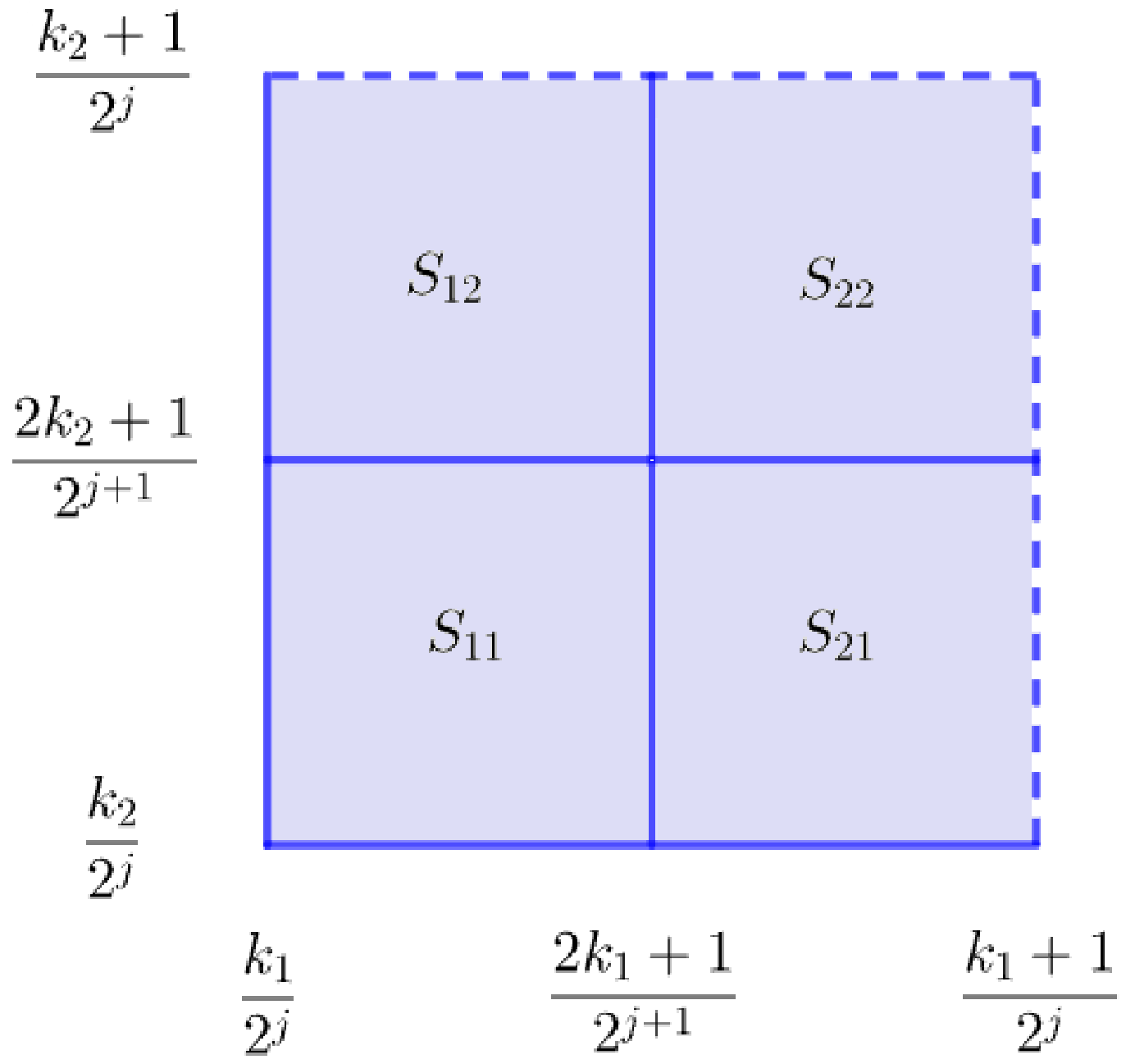
This square can be decomposed as a disjoint union of the following squares:

$$\begin{array}{cc}\hfill S_{11}(j,k_1,k_2)& =S(j+1,2k_1,2k_2),\hfill \\ \hfill S_{12}(j,k_1,k_2)& =S(j+1,2k_1,2k_2+1),\hfill \\ \hfill S_{21}(j,k_1,k_2)& =S(j+1,2k_1+1,2k_2),\hfill \\ \hfill S_{22}(j,k_1,k_2)& =S(j+1,2k_1+1,2k_2+1).\hfill \end{array}$$

Thus, we have that

$$\begin{array}{ccc}\hfill {\Phi }_{j,k_1,k_2}& =2^j{\chi }_{S_{11}},\hfill & \hfill {\Psi }_{j,k_1,k_2}^{(1,2)}=2^j\left({\chi }_{S_{11}\cup S_{21}}-{\chi }_{S_{12}\cup S_{22}}\right),\\ \hfill {\Psi }_{j,k_1,k_2}^{(2,1)}& =2^j\left({\chi }_{S_{11}\cup S_{12}}-{\chi }_{S_{21}\cup S_{22}}\right),\hfill & \hfill {\Psi }_{j,k_1,k_2}^{(2,2)}=2^j\left({\chi }_{S_{11}\cup S_{22}}-{\chi }_{S_{12}\cup S_{21}}\right),\end{array}$$

where the sets $S_{ij}$, with $i,i=1,2$, are illustred in Figure 1.

Consequently, for $f\in L^2\left({\mathbb{R}}^2\right)$ the operator ${\mathbf{P}}_{j}f$ acts as a discretization of f that is constant over the disjoint squares $S(j,k_1,k_2)$. For more details on the fundamental results in multiresolution analysis, see the following works: [9,10,11,13].

Additionally, let X be a compact subset of ${\mathbb{R}}^2$. We assume that $\mu$ is a measure absolutely continuous with respect to the Lebesgue measure $\lambda$, whose Radon-Nikodym derivative $f_{\mu }$ satisfies $f_{\mu }\in L^1\left(X\right)\cap L^2\left(X\right)$.

It is well known that ${\parallel {\mathbf{P}}_j{f}_{\mu }-f_{\mu }\parallel }_2\to 0$ as $j\to \infty$. Moreover, by the compactness of X, we have the estimate

$${\parallel {\mathbf{P}}_j{f}_{\mu }-f_{\mu }\parallel }_1\le \lambda {\left(X\right)}^{1/2}{\parallel {\mathbf{P}}_j{f}_{\mu }-f_{\mu }\parallel }_2.$$

Therefore, the approximation ${\mu }_j$ of the measure $\mu$ in the level j defined by $d{\mu }_j={\mathbf{P}}_j{f}_{\mu }d\lambda$ is absolutely continuous with respect to the Lebesgue measure $\lambda$. If we further assume that the measure $\mu$ has support contained in X, then the approximations ${\mu }_j$ converge to $\mu$ in both the $L^1$ and $L^2$ sense.

Note that for each ${\mu }_j$, there exists an integrable function ${\widehat{\mu }}_j\in {\mathbf{P}}_j{L}^2\left({\mathbb{R}}^2\right)$ such that ${\mu }_j\left(A\right)=\mathbb{E}\left[{\widehat{\mu }}_j{\chi }_A\right]$ for every Lebesgue measurable set $A\subset {\mathbb{R}}^2$, where $\mathbb{E}\left[g\right]$ denotes the expectation of g with respect to the Lebesgue measure.

Finally, the fact that each the measure ${\mu }_j$ has compact support implies that the sequence ${\left\{{\mu }_j\right\}}_{j\in \mathbb{Z}}$ converges weakly to the measure $\mu$. For further details on the approximation of a measure using multiresolution analysis, see [12,13].

3. Adjustment Automaton over Permutations

This section introduces a finite automaton defined on the permutation group $S_n$, designed to refine discretized feasible solutions to the Monge–Kantorovich (MK) problem. The automaton serves as a central tool in the subsequent section, where it enables systematic local adjustments that reduce the associated cost and thereby improves solution quality.

An automaton is a theoretical model of computation used to describe and analyze systems that process inputs and produce outputs according to a prescribed set of states and transition rules. Formally, an automaton is defined as follows:

Definition 1.

An automaton is defined as a 5-tuple:

$$A=(Q,\Sigma ,\delta ,q_0,F),$$

where:

• Q is a finite set of states,
• Σ is a finite set of input symbols called the alphabet,
• $\delta :Q\times \Sigma \to Q$ is the transition function,
• $q_0\in Q$ is the initial state,
• $F\subseteq Q$ is the set of accepting (or final) states.

Explanation of the Components:

1.

States (Q). At any given time, the automaton occupies one of a finite number of states. These states encode the internal configuration of the system and may be interpreted as its “memory.”

2.

Alphabet ($\Sigma$). The input alphabet is a finite set of symbols that the automaton is capable of reading. For instance, in the case of binary inputs, one has $\Sigma =\{0,1\}$.

3.

Transition Function ($\delta$). The transition function specifies how the automaton evolves from one state to another in response to an input symbol. Formally, it is a mapping

$$\delta :Q\times \Sigma \to Q.$$

Given a state $q\in Q$ and an input symbol $a\in \Sigma$, the value $\delta (q,a)$ determines the subsequent state of the automaton.

4.

Initial State ($q_0$). Computation begins at the distinguished initial state $q_0\in Q$, from which the automaton starts processing the input.

5.

Accepting States (F). A subset $F\subseteq Q$ is designated as the set of accepting (or final) states. An input string is said to be accepted by the automaton if, after the entire input has been processed, the automaton terminates in a state belonging to F.

Further information on the automaton is provided in [19,20]. We now recall the following concept:

Definition 2.

Let $n\in \mathbb{N}$ with $n\ne 0$, and let $\mathbf{n}=\{1,\dots ,n\}$. A permutation on n is an invertible function $\sigma :\mathbf{n}\to \mathbf{n}$. The set of all permutations on n, together with function composition, forms a group called the symmetric group of degree n, which is denoted by $S_n$.

A permutation $\sigma \in S_n$ can be represented as an array (or list) of length n, where the i-th entry specifies the image of i under $\sigma$. Formally, a permutation $\sigma$ is represented as:

$$\sigma =\left[\begin{array}{cccc}\sigma \left(1\right)& \sigma \left(2\right)& \dots & \sigma \left(n\right)\end{array}\right].$$

The inverse of a permutation $\sigma =\left[\begin{array}{cccc}\sigma \left(1\right)& \sigma \left(2\right)& \dots & \sigma \left(n\right)\end{array}\right]$ is the permutation ${\sigma }^{-1}$ such that:

$${\sigma }^{-1}\left(\sigma \left(i\right)\right)=i,\mathrm{for}\mathrm{all}i\in \{1,2,\dots ,n\}.$$

To compute ${\sigma }^{-1}$ from the array representation of $\sigma$, one swaps the indices and the corresponding values. A detailed discussion of permutations can be found in [21].

Example 1.

Let $\sigma =\left[\begin{array}{cccc}4& 3& 1& 2\end{array}\right]\in S_4$. Then its inverse permutation is given by

$${\sigma }^{-1}=\left[\begin{array}{cccc}3& 4& 2& 1\end{array}\right].$$

We can represent the permutation $\sigma$ by the matrix $A_{\sigma }={\left(a_{i,j}^{\sigma }\right)}_{i,j=1}^n$, defined by

$$a_{i,j}^{\sigma }=\left\{\begin{array}{cc}1,\hfill & \mathrm{if}j=\sigma \left(i\right),i=1,\dots ,n,\hfill \\ 0,\hfill & \mathrm{otherwise}.\hfill \end{array}\right.$$

(10)

Example 2.

Let $\sigma =\left[\begin{array}{ccc}3& 1& 2\end{array}\right]\in S_3$. Its matrix representation is given by

$$A_{\sigma }=\left[\begin{array}{ccc}0& 0& 1\\ 1& 0& 0\\ 0& 1& 0\end{array}\right].$$

Observe that for each fixed permutation $\sigma \in S_n$ and fixed index k, the components of $\sigma$ associated with the position k take the following form.

$$\begin{array}{cccccccc}\mathrm{values}& \sigma \left(k\right)-1& \cdots & \sigma (k-1)& \sigma \left(k\right)& \sigma (k+1)& \cdots & \sigma \left(k\right)+1\\ \mathrm{positions}& {\sigma }^{-1}(\sigma \left(k\right)-1)& \cdots & k-1& k& k+1& \cdots & {\sigma }^{-1}(\sigma \left(k\right)+1)\end{array}$$

The second row indicates the position in the array associated with the permutation $\sigma$, while k denotes the position at which the automaton acts.

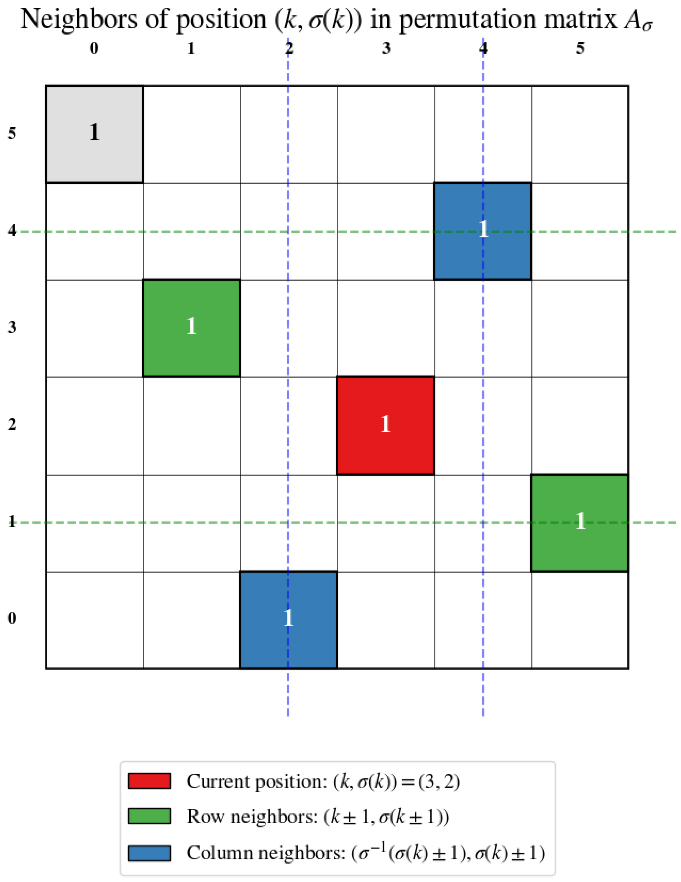
Example 3.

To exemplify the above paragraph, we consider the following permutation with respect to position $k=5$.

$$\begin{array}{cc}\sigma =& (4,6,8,7,2,5,3,1)\\ \mathit{positions}& 1,2,3,4,5,6,7,8\end{array}$$

The inverse permutation is given by

$$\begin{array}{cc}{\sigma }^{-1}=& (8,5,7,1,6,2,4,3)\\ \mathit{positions}& 1,2,3,4,5,6,7,8\end{array}$$

Now, calculate the distinguished position with respect to $k=5$, which are $4,5,6,7,8$ since

$${\sigma }^{-1}(\sigma \left(k\right)+1)={\sigma }^{-1}(\sigma \left(5\right)-1)={\sigma }^{-1}(2-1)=8,$$

and

$${\sigma }^{-1}(\sigma \left(k\right)+1)={\sigma }^{-1}(2+1)=7.$$

Finnally, the matrix representation is given by

$$A_{\sigma }=\left[\begin{array}{cccccccc}0& 0& 0& 1& 0& 0& 0& 0\\ 0& 0& 0& 0& 0& 1& 0& 0\\ 0& 0& 0& 0& 0& 0& 0& 1\\ 0& 0& 0& 0& 0& 0& 1& 0\\ 0& 1& 0& 0& 0& 0& 0& 0\\ 0& 0& 0& 0& 1& 0& 0& 0\\ 0& 0& 1& 0& 0& 0& 0& 0\\ 1& 0& 0& 0& 0& 0& 0& 0\end{array}\right].$$

Remark 1.

In the figures presented in Section 5, the graphs representing the permutations (feasible solutions) are numbered from bottom to top and from left to right. Moreover, the positions of the 1’s are represented by colored points. In contrast, in the previous matrix representation, the numbering is carried out from top to bottom and from right to left. For example, considering the row reordering used in Section 5, the previous matrix corresponds to the following arrangement.

$$\left[\begin{array}{cccccccc}1& 0& 0& 0& 0& 0& 0& 0\\ 0& 0& 1& 0& 0& 0& 0& 0\\ 0& 0& 0& 0& 1& 0& 0& 0\\ 0& 1& 0& 0& 0& 0& 0& 0\\ 0& 0& 0& 0& 0& 0& 1& 0\\ 0& 0& 0& 0& 0& 0& 0& 1\\ 0& 0& 0& 0& 0& 1& 0& 0\\ 0& 0& 0& 1& 0& 0& 0& 0\end{array}\right].$$

Finally, the representation of the permutation using colored points is as follows:

$$\left[\begin{array}{cccccccc}•& & & & & & & \\ & & •& & & & & \\ & & & & •& & & \\ & •& & & & & & \\ & & & & & & •& \\ & & & & & & & •\\ & & & & & •& & \\ & & & •& & & & \end{array}\right].$$

The neighbors’ interpretation is as follows. The neighbors of $(k,\sigma (k\left)\right)$ in the matrix representation are those positions that contain the value 1 in the rows and columns adjacent to position $(k,\sigma (k\left)\right)$, since $\sigma$ is fixed, we will refer to the position $(k,\sigma (k\left)\right)$ simply as position k. Explicitly, these positions are:

$$\begin{array}{cc}\hfill \left({\sigma }^{-1}(\sigma \left(k\right)-1),\sigma \left(k\right)-1\right),& \left(k-1,\sigma (k-1)\right),\hfill \\ \hfill \left(k+1,\sigma (k+1)\right),& \left({\sigma }^{-1}(\sigma \left(k\right)+1),\sigma \left(k\right)+1\right)\hfill \end{array}$$

For simplicity, we will write

$${\sigma }^{-1}(\sigma \left(k\right)-1),k-1,k+1,{\sigma }^{-1}(\sigma \left(k\right)+1)$$

to denote the neighbors of position k, which are illustrated in Figure 2.

Definition 3.

We define an adjusted automaton constructed from the elements of $S_n$ in the following manner: we consider the 5-tuple

$$A=(Q,\Sigma ,\delta ,q_0,F),$$

(11)

where:

• $Q=S_n\times \{1,\dots ,n+1\}$ is a finite set of states,
• $\Sigma =\{0,1,2,3,4\}$ is a finite set of input symbols called the alphabet,
• $\delta :Q\times \Sigma \to Q$ is the transition function, which is defined by

  $$\begin{array}{c}\hfill \delta \left(\right(\sigma ,k),0)=(\sigma ,k+1)\\ \hfill \delta ((\sigma ,k),1)=({\sigma }_1,k+1)\\ \hfill \delta ((\sigma ,k),2)=({\sigma }_2,k+1)\\ \hfill \delta ((\sigma ,k),3)=({\sigma }_3,k+1)\\ \hfill \delta ((\sigma ,k),4)=({\sigma }_4,k+1)\end{array}$$

  where

  $$\begin{array}{c}{\sigma }_1=\left[\sigma \left(1\right),\dots \sigma \left(k\right)-1,\dots ,\sigma \left(k\right),\sigma (k-1),\sigma (k+1),\dots ,\sigma \left(k\right)+1,\dots ,\sigma \left(n\right)\right]\hfill \\ {\sigma }_2=[\sigma \left(1\right),\dots ,\sigma \left(k\right)-1,\dots ,\sigma (k-1),\sigma (k+1),\sigma \left(k\right)\dots ,\sigma \left(k\right)+1,\dots ,\sigma \left(n\right)]\hfill \\ {\sigma }_3=[\sigma \left(1\right),\dots ,\sigma \left(k\right),\dots \sigma (k-1),\sigma \left(k\right)-1,\sigma (k+1),\dots ,\sigma \left(k\right)+1,\dots ,\sigma \left(n\right)]\hfill \\ {\sigma }_4=[\sigma \left(1\right),\dots ,\sigma \left(k\right)-1,\dots \sigma (k-1),\sigma \left(k\right)+1,\sigma (k+1),\dots ,\sigma \left(k\right),\dots ,\sigma \left(n\right)]\hfill \end{array}$$
• $q_0=({\sigma }_0,1)\in Q$ is the initial state, where ${\sigma }_0$ is any element of $S_n$.
• $F=S_n\times \{n+1\}\subseteq Q$ is the set of accepting (or final) states.

4. Improving Solutions of the Monge–Kantorovich Problem via an Adjustment Automaton on the Permutation Group

In this section, we present a hybrid methodology that integrates Haar wavelet-based multiresolution analysis (MRA) with a finite automaton acting on permutations, with the aim of obtaining optimal solutions to the Monge–Kantorovich (MK) problem.

This approach exploits the hierarchical structure of MRA to construct an initial approximate solution, which is subsequently refined through local adjustments performed by the automaton described in the previous section.

M-K Problem and MRA

A measure $\mu \in M^{+}(X\times Y)$ is said to be a feasible solution to the $\mathrm{MK}$ problem if it satisfies (3) and the pairing $\langle \mu ,c\rangle$ is finite. The $\mathrm{MK}$ problem is said to be solvable if there exists a feasible measure ${\mu }^{*}$ that attains the optimal value of the objective functional. In this case, ${\mu }^{*}$ is referred to as an optimal solution of (3).

Moreover, assuming that $\mu$ is absolutely continuous with respect to the Lebesgue measure on ${\mathbb{R}}^2$ and that ${\eta }_1$ and ${\eta }_2$ are absolutely continuous with respect to the Lebesgue measure on $\mathbb{R}$, the $\mathrm{MK}$ problem admits a natural discretization via Haar multiresolution analysis on ${\mathbb{R}}^2$.

Recall that, according to Equation (3), the Monge–Kantorovich problem at level j is given by:

$$\begin{array}{cc}\hfill {\mathrm{MK}}_j:\mathrm{minimize}& {\displaystyle \langle {\mu }_j,c\rangle :=\int cd{\mu }_j}\hfill \\ \hfill \mathrm{subject}\mathrm{to}:& {\Pi }_1{\mu }_j\left(E_1\right)={\eta }_j^1\left(E_1\right),{\Pi }_2{\mu }_j\left(E_2\right)={\eta }_j^2\left(E_2\right),\mu \in M^{+}(X\times Y),\hfill \end{array}$$

for each $\mu$-measurable set $E_1\subset X$ and $E_2\subset Y$, where ${\mu }_j$, ${\eta }_j^1$ and ${\eta }_j^2$ are the projections to level j of the measures $\mu$, ${\eta }^1$ and ${\eta }^2$ to the respective Haar MRA.

In particular, we consider the $\mathrm{MK}$ problem with cost function $c=c(x,y)$, base sets $X=Y=[0,1]$, and marginal measures ${\eta }^1={\eta }^2{=\lambda |}_{[0,1]}$. Since practical applications typically involve discretized formulations, the application of multiresolution analysis on ${\mathbb{R}}^2$ leads us to the following objective problem:

$$\begin{array}{cc}\hfill {\mathrm{MK}}_j:\mathrm{minimize}& {\displaystyle \sum _{i,k}{\mu }_{i,k}^j{c}_{i,k}^j}\hfill \\ \hfill \mathrm{subject}\mathrm{to}:& {\displaystyle \sum _i{\mu }_{i,k}^j=\frac{1}{2^j},\mathrm{for}\mathrm{each}k=1,\dots ,2^j.}\hfill \\ \hfill & {\displaystyle \sum _k{\mu }_{i,k}^j=\frac{1}{2^j},\mathrm{for}\mathrm{each}i=1,\dots ,2^j.}\hfill \\ \hfill & {\displaystyle \sum _{i,k}{\mu }_{i,k}^j=1.}\hfill \\ \hfill & {\mu }_{i,k}^j\ge 0,\mathrm{for}\mathrm{each}i,k=1,\dots ,2^j.\hfill \end{array}$$

(12)

Here, ${\mu }_{i,k}^j$ denotes the portion of the initial mass ${\displaystyle \frac{1}{2^j}}$ located at the interval $I_{j,i}$ on the x-axis that is allocated to the interval $I_{j,k}$ on the y-axis. We refer to the j-discrete unit square as the grid formed by the squares $S(j,k_1,k_2)$ (see (9)), which partitions the set $[0,1]\times [0,1]$ into $2^j\times 2^j$ blocks, each naturally identified with the point $(k_1,k_2)$.

The above formulation is an assignment problem, which is a particular case of the transport problem. The problem instance has a number of agents and a number of tasks. Any agent can be assigned to perform any task, incurring some cost that may vary depending on the agent-task assignment. The Hungarian method is a combinatorial optimization algorithm that solves the assignment problem in polynomial time and which anticipated later primal–dual methods. It was developed and published in 1955 by Harold Kuhn, who gave it the name “Hungarian method” because the algorithm was largely based on the earlier works of two Hungarian mathematicians, Dénes Kőnig and Jenő Egerváry. For more details, see [15,16,17].

We assume the existence of a simple solution $\mu$ to (12). That is, $\mu$ is a feasible solution such that, for any $i_0,k_0\in \{1,\dots ,2^j\}$ with ${\mu }_{i_0,k_0}\ne 0$, it necessarily holds that ${\mu }_{i_0,k}=0$ for all $k\ne k_0$ and ${\mu }_{i,k_0}=0$ for all $i\ne i_0$.

All feasible solutions of (12) correspond to permutations $\sigma \in S_{2^j}$. Consequently, we employ the automaton introduced in Section 3, with $n=2^j$ in this setting.

Our objective is to improve a given solution of (12), where $c_{i,k}^j$ denotes the associated cost matrix. Based on this cost matrix and the current state of the automaton, we introduce the following quantities.

$$\begin{array}{cc}\hfill a_1& =c_{k-1,\sigma (k-1)}^j+c_{k,\sigma \left(k\right)}^j-c_{k,\sigma (k-1)}^j-c_{k-1,\sigma \left(k\right)}^j\hfill \\ \hfill a_2& =c_{k+1,\sigma (k+1)}^j+c_{k,\sigma \left(k\right)}^j-c_{k,\sigma (k+1)}^j-c_{k+1,\sigma \left(k\right)}^j\hfill \\ \hfill a_3& =c_{{\sigma }^{-1}(\sigma \left(k\right)-1),\sigma \left(k\right)-1}^j+c_{k,\sigma \left(k\right)}^j-c_{k,\sigma \left(k\right)-1}^j-c_{{\sigma }^{-1}(\sigma \left(k\right)-1),\sigma \left(k\right)}^j\hfill \\ \hfill a_4& =c_{{\sigma }^{-1}(\sigma \left(k\right)+1),\sigma \left(k\right)+1}^j+c_{k,\sigma \left(k\right)}^j-c_{k,\sigma \left(k\right)+1}^j-c_{{\sigma }^{-1}(\sigma \left(k\right)+1),\sigma \left(k\right)}^j\hfill \end{array}$$

(13)

Definition 4.

We define the evaluation function of the state associated with the matrix $c_{i,k}^j$ as follows:

$$\begin{array}{c}\hfill f\left((\sigma ,k)\right)=\left\{\begin{array}{cc}0& \mathit{If}{a}_1\le 0,a_2\le 0,a_3\le 0,a_4\le 0,\hfill \\ 1& \mathit{If}{a}_1\ge 0,a_1\ge a_2,a_1\ge a_3,a_1\ge a_4,\hfill \\ 2& \mathit{If}{a}_2\ge 0,a_2\ge a_1,a_2\ge a_3,a_2\ge a_4,\hfill \\ 3& \mathit{If}{a}_3\ge 0,a_3\ge a_1,a_3\ge a_2,a_3\ge a_4,\hfill \\ 4& \mathit{If}{a}_4\ge 0,a_4\ge a_1,a_4\ge a_2,a_4\ge a_3.\hfill \end{array}\right.\end{array}$$

(14)

where the values $a_j$ for $j=0,\dots ,5$ are given by (13).

The interpretation of the evaluation function is the following:

• If $f\left((\sigma ,k)\right)=0$ then any change improves the feasible solution.
• If $f\left((\sigma ,k)\right)=1$ then the change in the positions $k-1$ and k (in the array representation of $\sigma$) is the better local change that improves the feasible solution.
• If $f\left((\sigma ,k)\right)=2$ then the change in the positions $k+1$ and k is the better local change that improves the feasible solution.
• If $f\left((\sigma ,k)\right)=3$ then the change in the positions ${\sigma }^{-1}\left(\sigma \left(k\right)-1\right)$ and k is the better local change that improves the feasible solution.
• If $f\left((\sigma ,k)\right)=4$ then the change in the positions ${\sigma }^{-1}\left(\sigma \left(k\right)+1\right)$ and k is the better local change that improves the feasible solution.

By construction, if we consider a state $({\sigma }_k,k)$ and apply the automaton with the alphabet symbol $f({\sigma }_k,k)$, we obtain the following.

$$\delta \left(({\sigma }_k,k),f({\sigma }_k,k)\right)=({\sigma }_{k+1},k+1).$$

It is clear that both ${\sigma }_k$ and ${\sigma }_{k+1}$ are feasible solutions of (12). Moreover, by construction of function f defined in (14), we have

$$\sum _{i,l=1}^{2^{-j}}{2}^{-j}{a}_{i,l}^{{\sigma }_{k+1}}{c}_{i,l}^j\le \sum _{i,l=1}^{2^{-j}}{2}^{-j}{a}_{i,l}^{{\sigma }_k}{c}_{i,l}^j,$$

equivalently

$$\sum _{l=1}^{2^{-j}}{2}^{-j}{c}_{l,{\sigma }_{k+1}\left(l\right)}^j\le \sum _{l=1}^{2^{-j}}{2}^{-j}{c}_{l,{\sigma }_k\left(l\right)}^j,$$

where $a_{i,l}^{{\sigma }_k}$ and $a_{i,l}^{{\sigma }_{k+1}}$ denote the entries of the matrices associated with ${\sigma }_k$ and ${\sigma }_{k+1}$, respectively, as defined in (10).

In summary, we have the following result.

Theorem 1.

Consider the transport problem given by (12) and consider a state $({\sigma }_k,k)$ where ${\sigma }_k$ is a permutation and a feasible solution of the transport problem. Let f be a function that evaluates a state with respect to a cost matrix given by (14). If $\delta ((\sigma ,k),f({\sigma }_k,k))=({\sigma }_{k+1},k+1)$, then

$$\sum _{i,k}^{2^{-j}}{2}^{-j}{a}_{i,k}^{{\sigma }_{k+1}}{c}_{i,k}^j\le \sum _{i,k}^{2^{-j}}{2}^{-j}{a}_{i,k}^{{\sigma }_k}{c}_{i,k}^j.$$

equivalently

$$\sum _l^{2^{-j}}{2}^{-j}{c}_{l,{\sigma }_{k+1}\left(l\right)}^j\le \sum _l^{2^{-j}}{2}^{-j}{c}_{l,{\sigma }_k\left(l\right)}^j.$$

Given an initial state of the automata $({\sigma }_0,1)$, we applied the automata to improve the feasible solution ${\sigma }_0$ as follows.

$$\begin{array}{cc}\hfill \delta (({\sigma }_0,1),f({\sigma }_0,1))& =({\sigma }_1,2)\hfill \\ \hfill \delta (({\sigma }_1,2),f({\sigma }_1,2))& =({\sigma }_2,3)\hfill \\ \hfill & ⋮\hfill \\ \hfill \delta (({\sigma }_{2^j-1},2^j),f({\sigma }_{2^j-1},2^j))& =({\sigma }_{2^j},2^j+1).\hfill \end{array}$$

Thus, we find that the final state of the automaton is given by $({\sigma }_{2^j},2^j+1)$. Therefore, the final state ${\sigma }_{2^j}$ of the automaton provides an improved solution compared to the initial state ${\sigma }_0$.

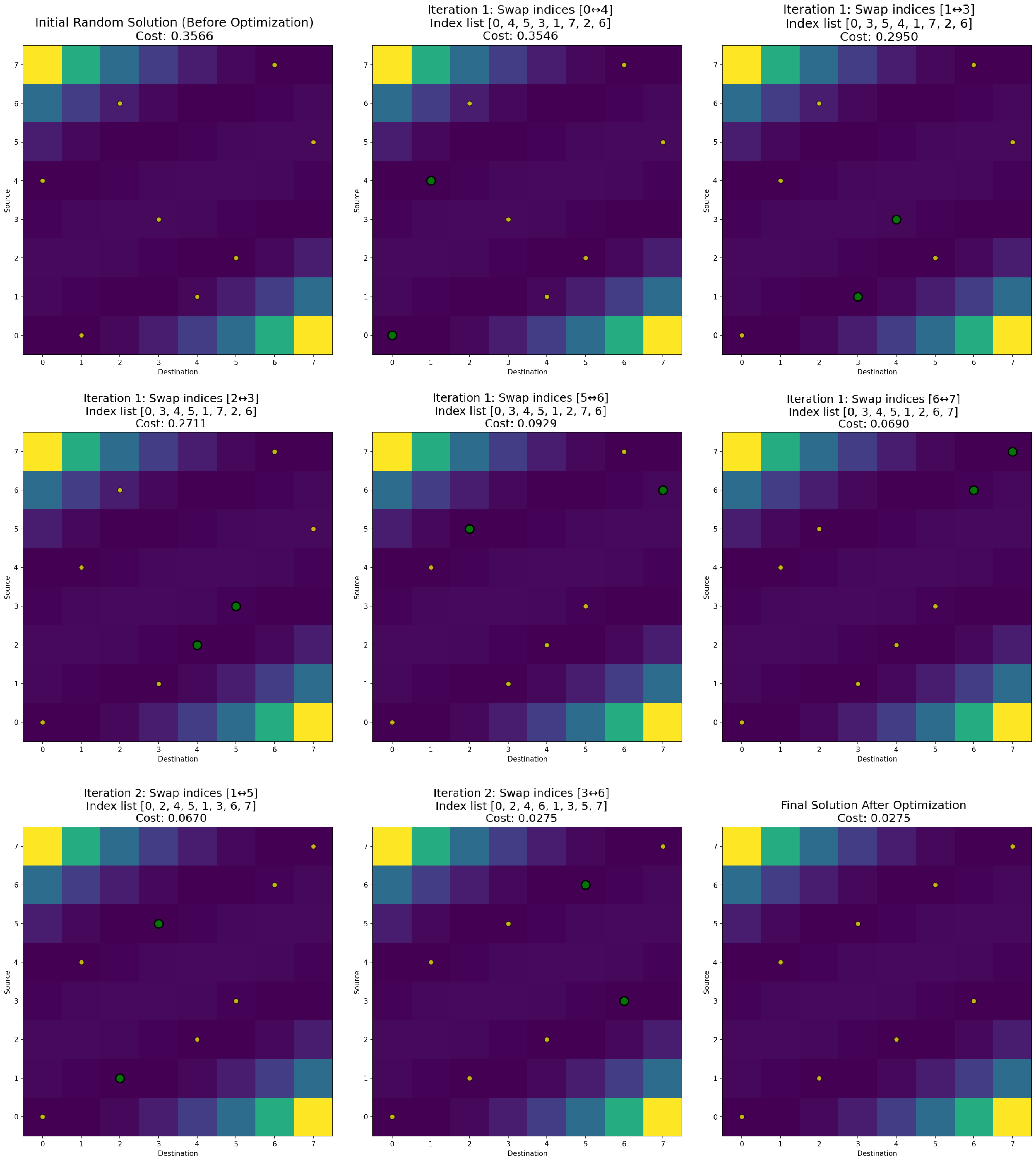
Example 4.

Figure 3 illustrates the application of the tuning automaton to the Monge–Kantorovich problem with cost function ${(2y-x-1)}^2{(2y-x)}^2$, discretized at level 3, which produces a cost matrix of size $8\times 8$.

The first image corresponds to a randomly generated feasible solution, obtained from a random permutation. The remaining images show the successive adjustments performed by the automaton as it evaluates possible swaps between neighboring elements.

In each step, the colored markers indicate the candidate solution under evaluation. The green dots represent the elements involved in the swap currently being tested, while the yellow dots correspond to assignments that remain fixed during that evaluation step.

The evaluation process proceeds sequentially by rows. Starting from row 0, the algorithm evaluates possible exchanges with neighboring elements; the process then continues with row 1, and so on until all rows have been examined.

The last image corresponds to the optimal solution obtained using the Hungarian algorithm. In this example, the solution produced by the proposed automaton coincides with the optimal solution.

5. Examples of the Proposed Methodology Based on Wavelets and an Automaton

The automaton constitutes a viable alternative for improving feasible solutions. Nevertheless, it is desirable for its initial state to be a feasible solution to the Monge–Kantorovich problem that already provides a close approximation to the optimal solution. To construct such an initial solution, we adopt the first stage of the scheme proposed in [13], which is then used as the input for the automaton.

Our approximation scheme consists of the following steps:

1.

Discretization of the cost function: The cost function is discretized at level j, and the resulting discretized cost is denoted by $c_j$.

2.

Application of the wavelet transform: Applying the wavelet transform to $c_j$, we obtain:

• a low-pass component, denoted by $c_{j-1}$;
• three high-pass components, denoted by ${\Psi }_1$, ${\Psi }_2$, and ${\Psi }_3$.

3.

Solution of the $M{K}^{j-1}$ problem: Using the cost function $c_{j-1}$ and the methodology proposed in [12], we compute an optimal solution ${\mu }_{j-1}^{*}$ to the $M{K}^{j-1}$ problem.

4.

Feasible solution construction for $M{K}^j$ problem: Using ${\mu }_{j-1}^{*}$ together with the high-pass components ${\Psi }_1$, ${\Psi }_2$, and ${\Psi }_3$, we construct a feasible solution ${\widehat{\mu }}_j$ at level j with the following properties:

(a)

  ${\mathbf{P}}_{j-1}\left({\widehat{\mu }}_j\right)={\mu }_{j-1}^{*}$

(b)

  ${\mathbf{Q}}_{j-1}^{(1,2)}\left({\widehat{\mu }}_j\right)=0$

(c)

  ${\mathbf{Q}}_{j-1}^{(2,1)}\left({\widehat{\mu }}_j\right)=0$

(d)

  ${\mathbf{Q}}_{j-1}^{(2,2)}\left({\widehat{\mu }}_j\right)=\mathrm{sign}\left({\Psi }_3\right){\mu }_{j-1}^{*}$.

Here, $sign(·)$ denotes the sign function. In other words, the support of ${\widehat{\mu }}_j$ is contained in the support of ${\mu }_{j-1}^{*}$. The components ${\Psi }_1$ and ${\Psi }_2$ do not participate in the construction, as they affect the boundary conditions of the $M{K}^j$ problem. Finally, the sign of ${\Psi }_3$ determines the direction in which the solution is scaled.

5.

Implementation of the automaton: We use the feasible solution ${\widehat{\mu }}_j$ as the input to the automaton defined in (11). The automaton’s output yields the final approximation.

5.1. Example 1

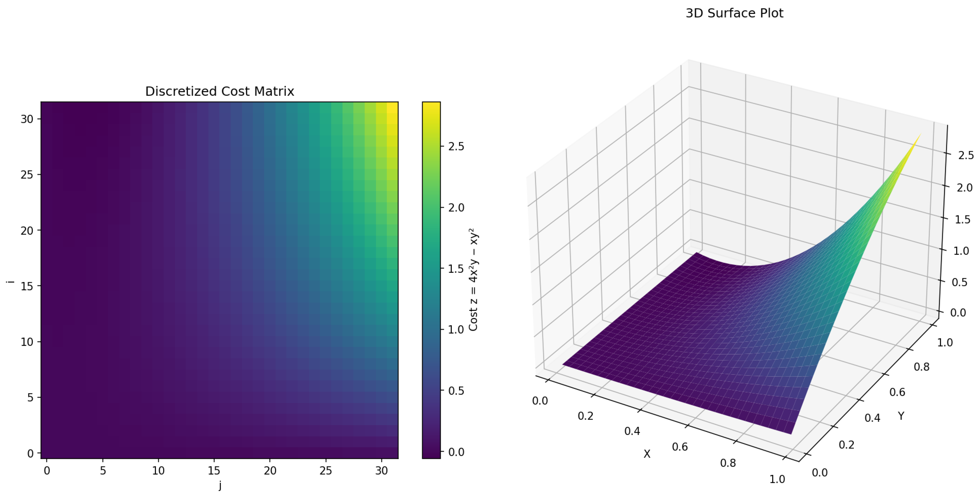
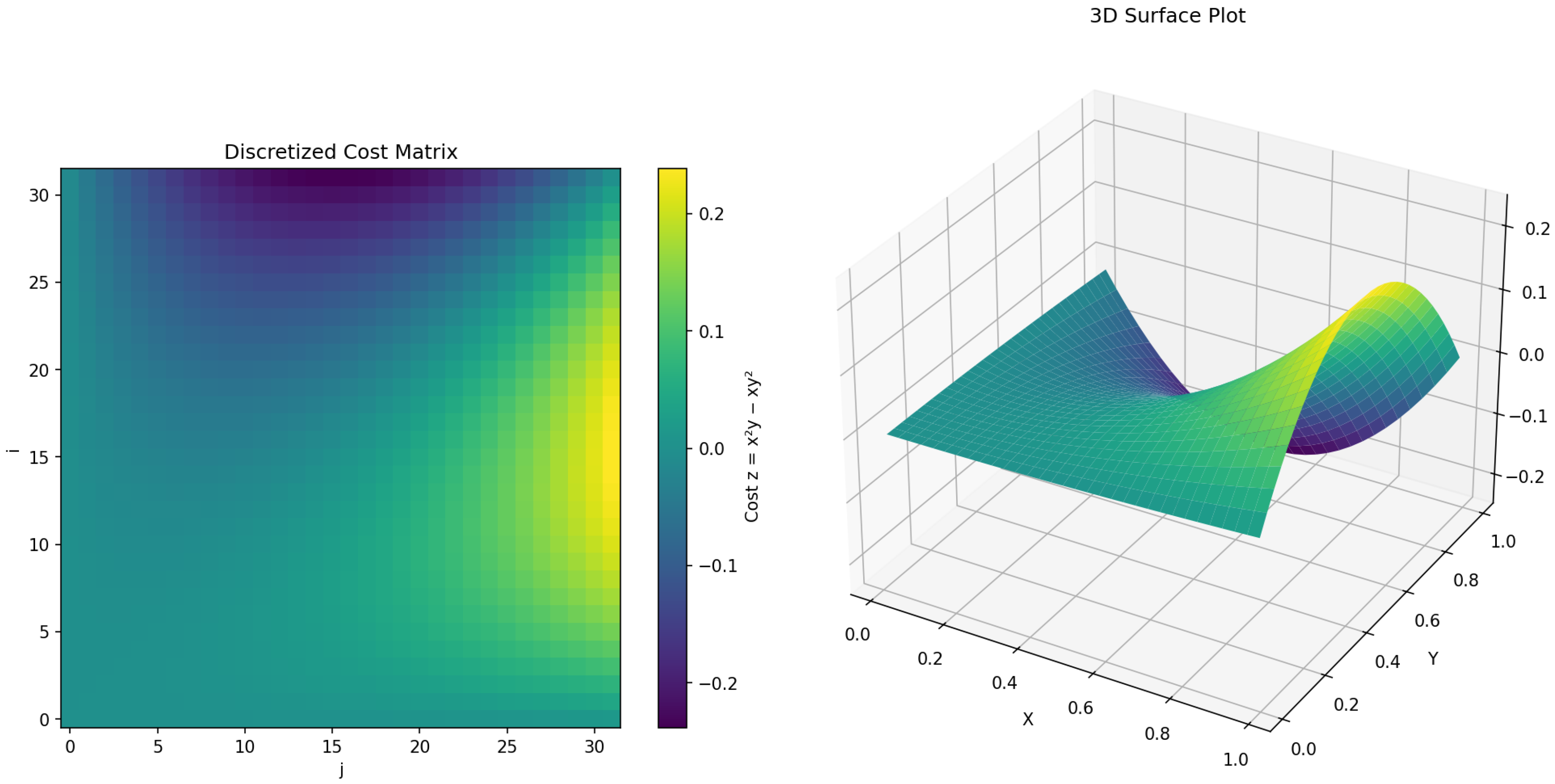
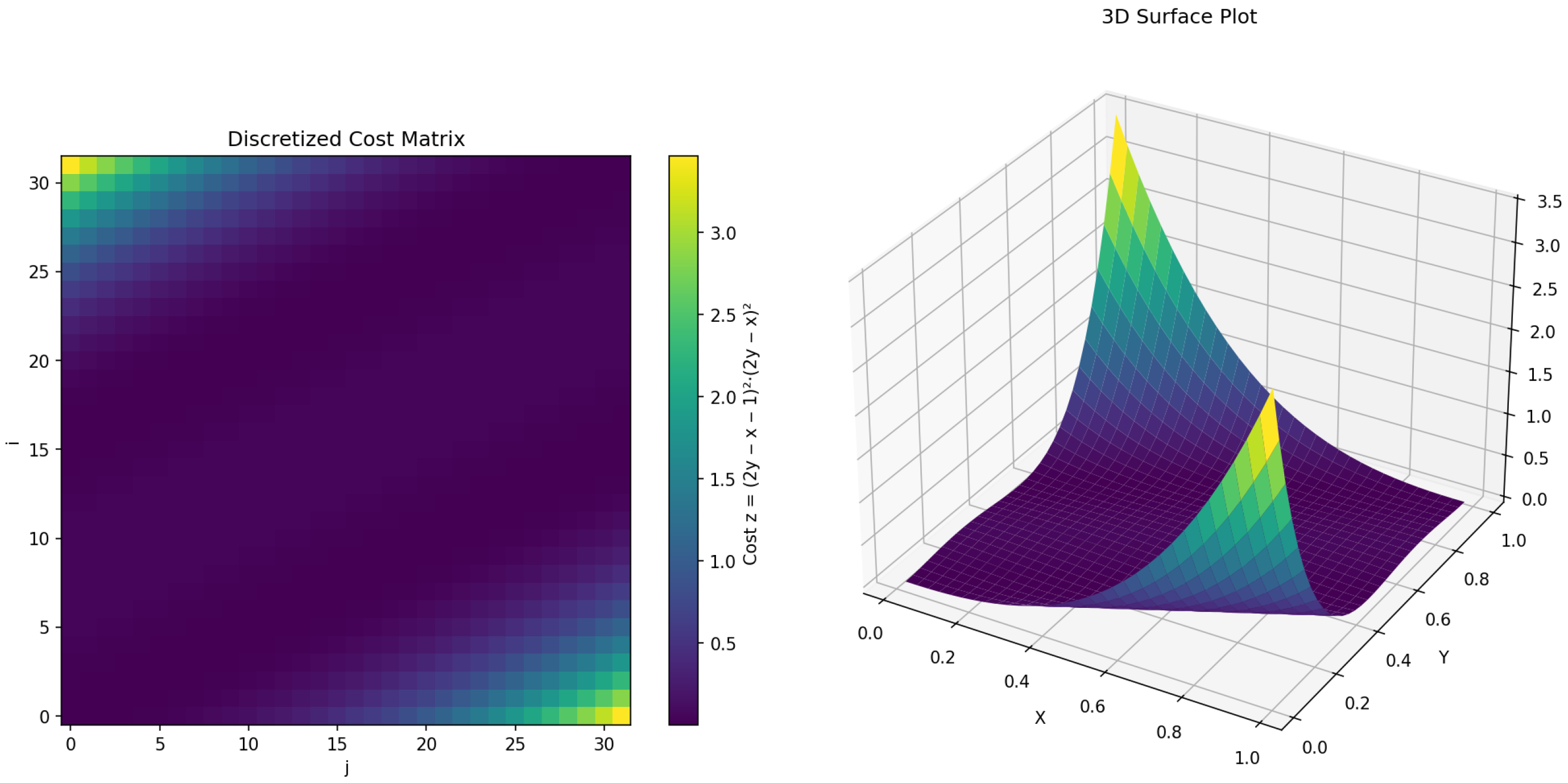
In this example, we consider the cost function $4x^{2}y-x{y}^2$. In Figure 4, the left side represents the discretization for level 5, where the cost function turns out on a cost matrix of $32\times 32$, and the right side represents 3-dimensional graphics of the cost function.

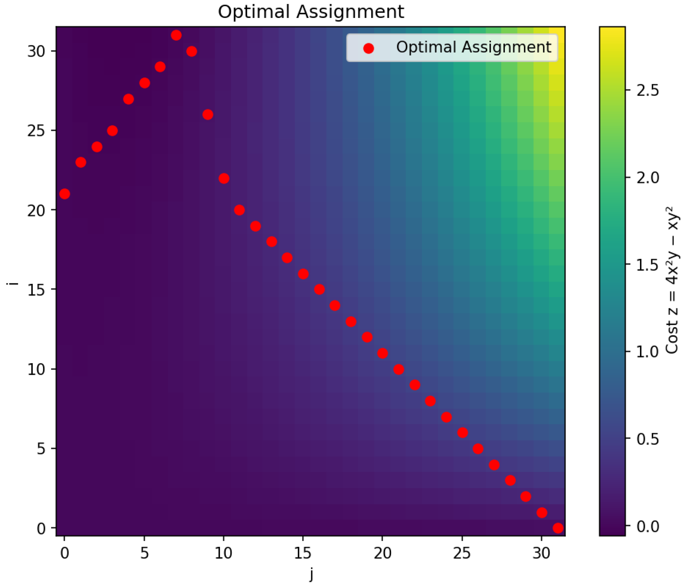
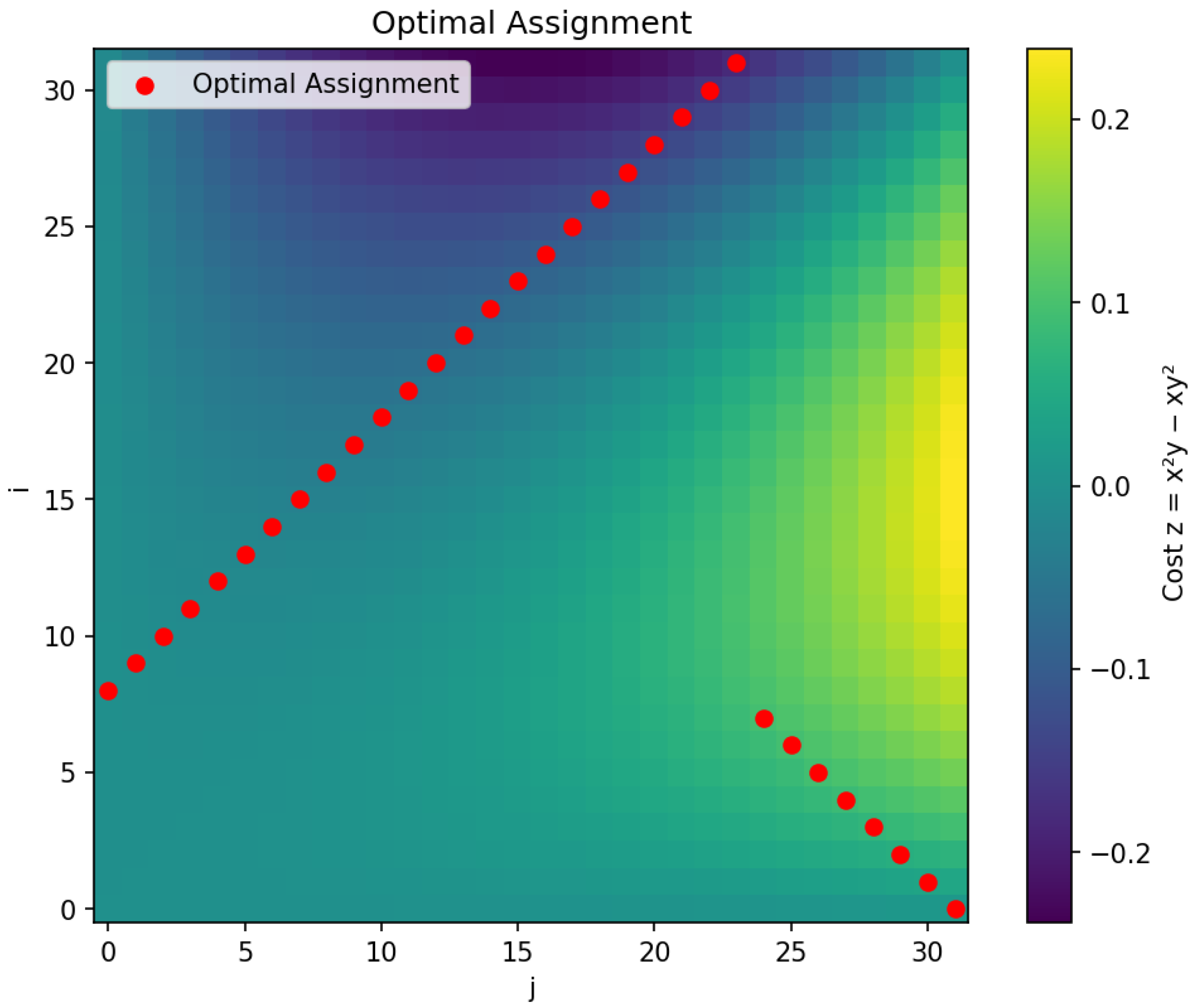
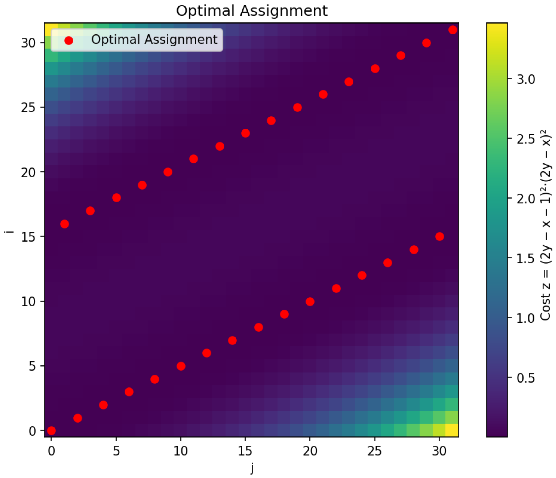
According to [12], the optimal solution ${\mu }_5$ at this level is illustrated in Figure 5, where the red points indicate the optimal assignments of the transportation problem.

Below, we present the implementation of the algorithm described at the beginning of this section.

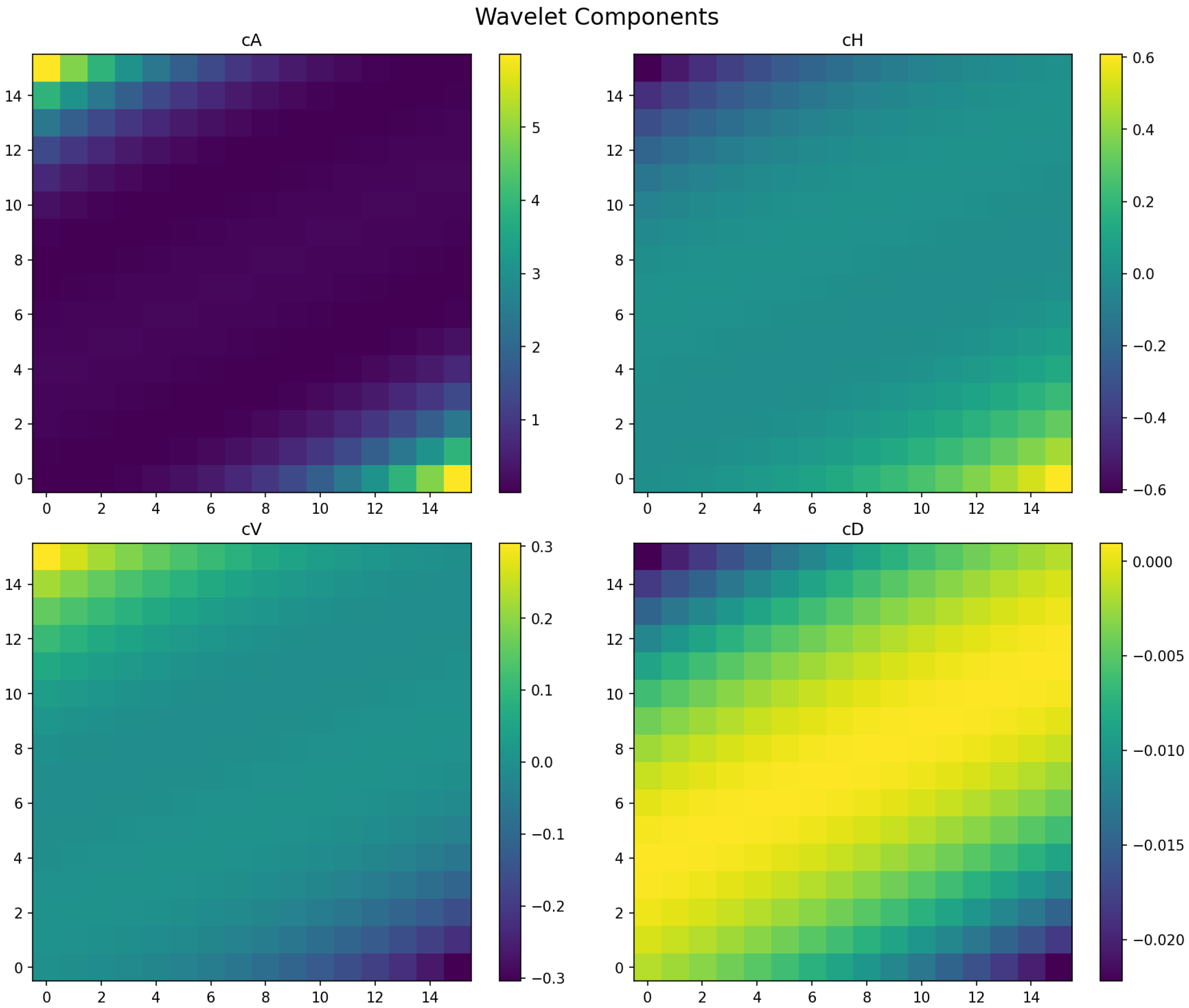
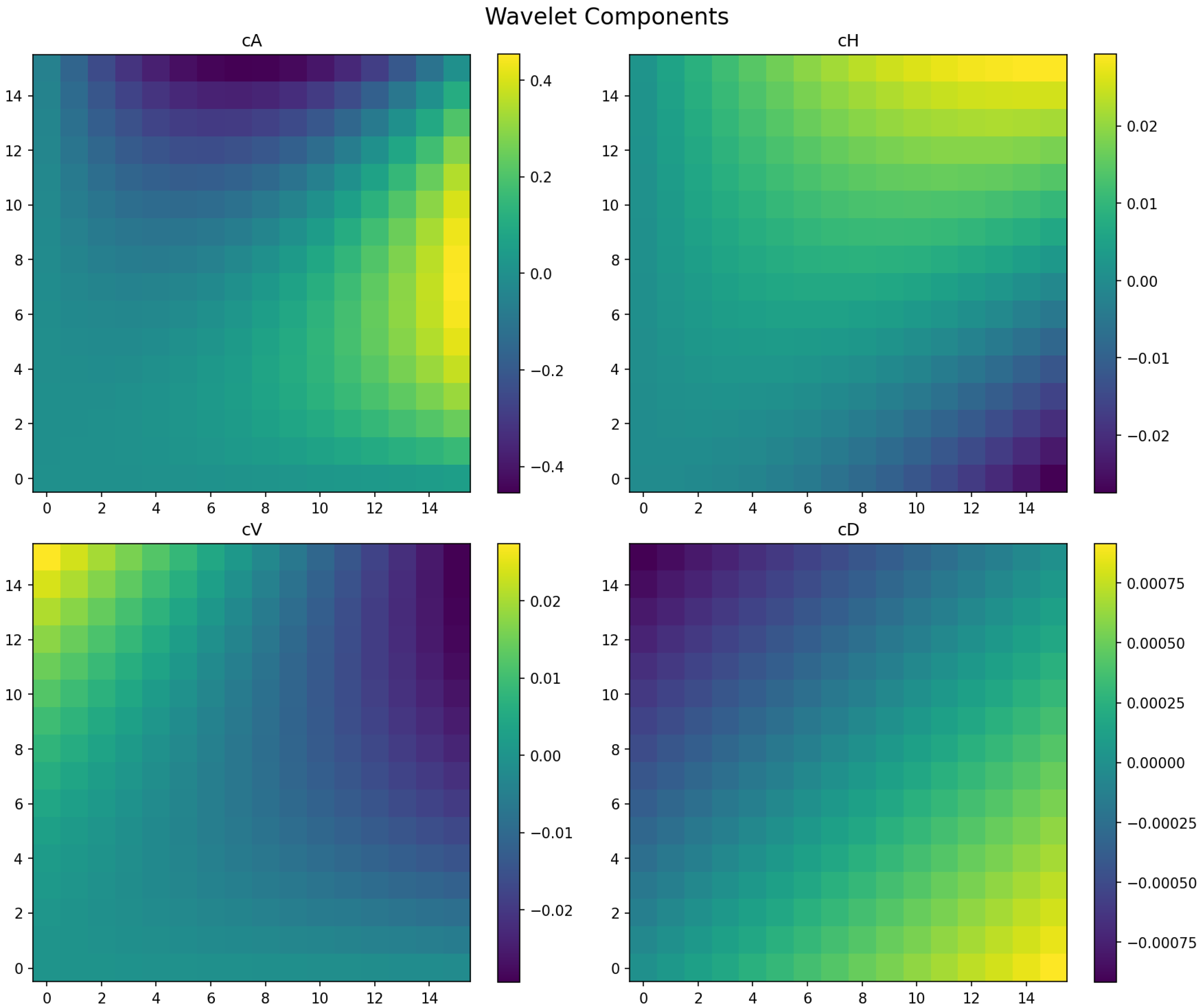
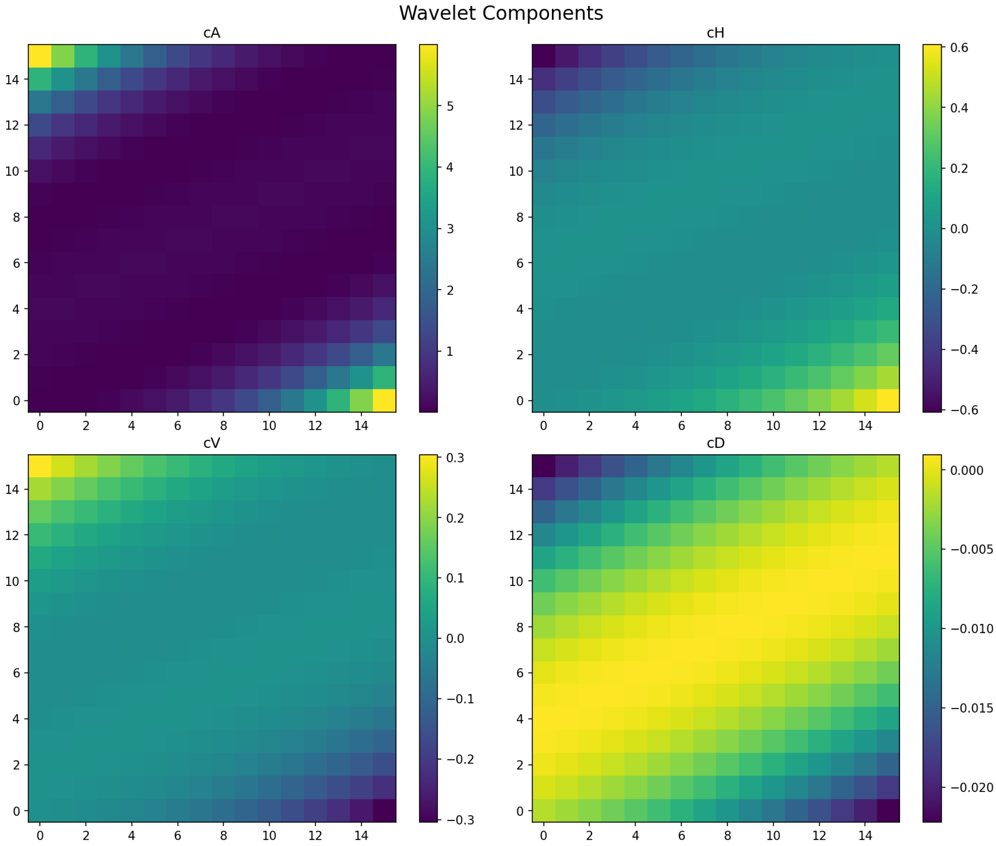
Applying the wavelet transform to the previous function, we obtain the decomposition in Figure 6.

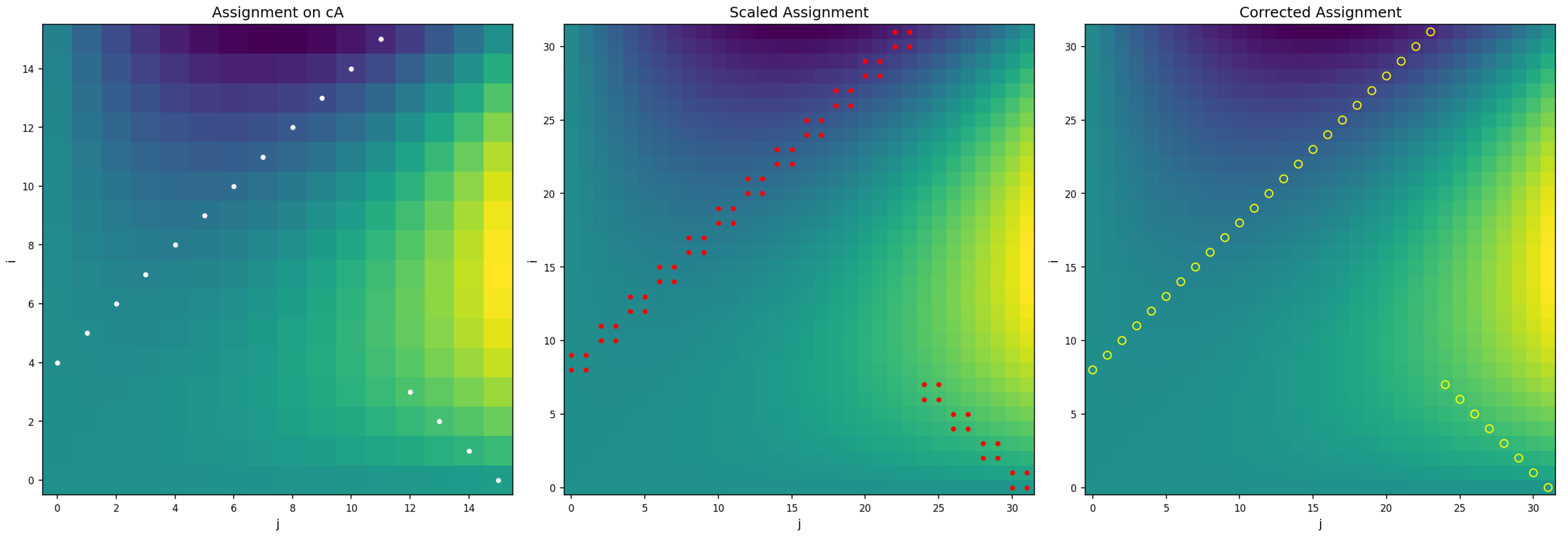
Here, the upper-left figure illustrates the lower-level approximation, the upper-right figure depicts the horizontal details, the lower-left figure shows the vertical details, and the lower-right figure corresponds to the diagonal details.

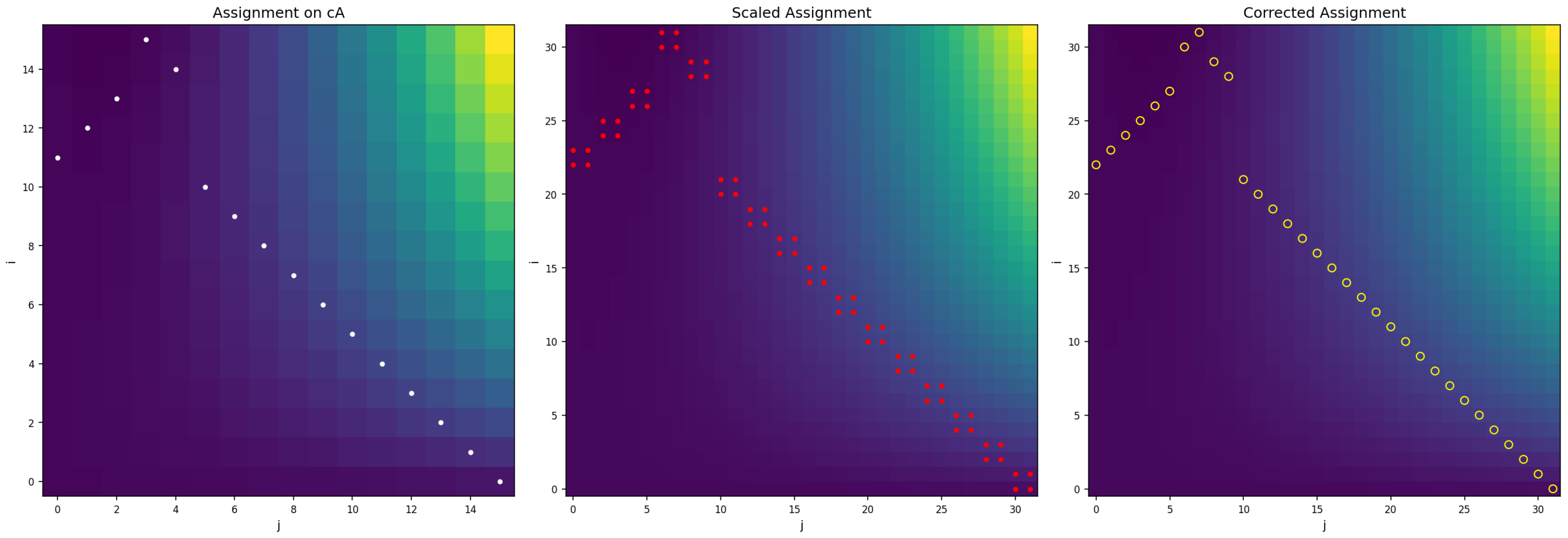
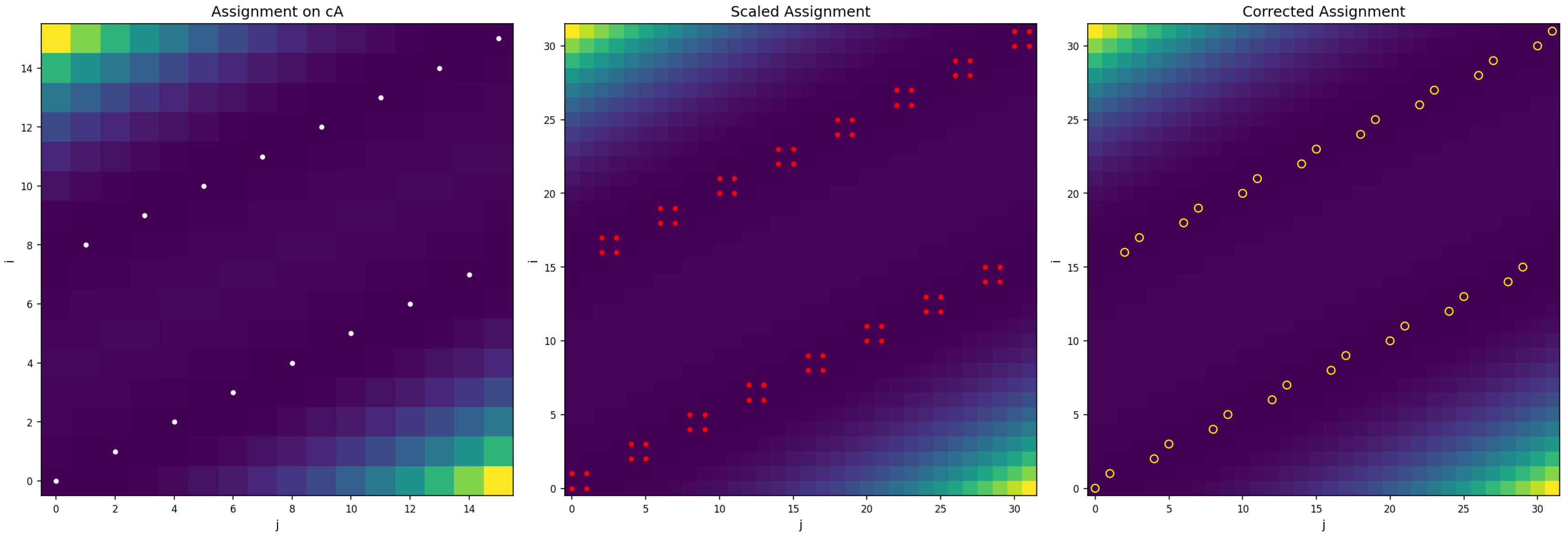
By solving the transportation problem for the cost function given by the approximation at the lower level, we obtain the measure ${\mu }_4^{*}$. The goal is to construct a feasible solution ${\widehat{\mu }}_5$ (level 5) from ${\mu }_4^{*}$ and the components ${\Psi }_1$, ${\Psi }_2$, and ${\Psi }_3$, as illustrated in Figure 7.

Description of Figure 7.

• The figure on the left depicts the optimal solution to the transportation problem (${\mu }_4^{*}$), where the cost matrix is obtained from the wavelet-based approximation shown in the upper-left panel of Figure 6.
• The central figure represents the natural extension of this solution to a higher level; however, it does not constitute a feasible solution to the transportation problem.
• The figure on the right shows a feasible solution to the transportation problem at the higher level. This solution is obtained by selecting one diagonal from each $2\times 2$ block in the central figure, with the choice guided by the sign of the diagonal detail matrix (see the lower-right panel of Figure 6).

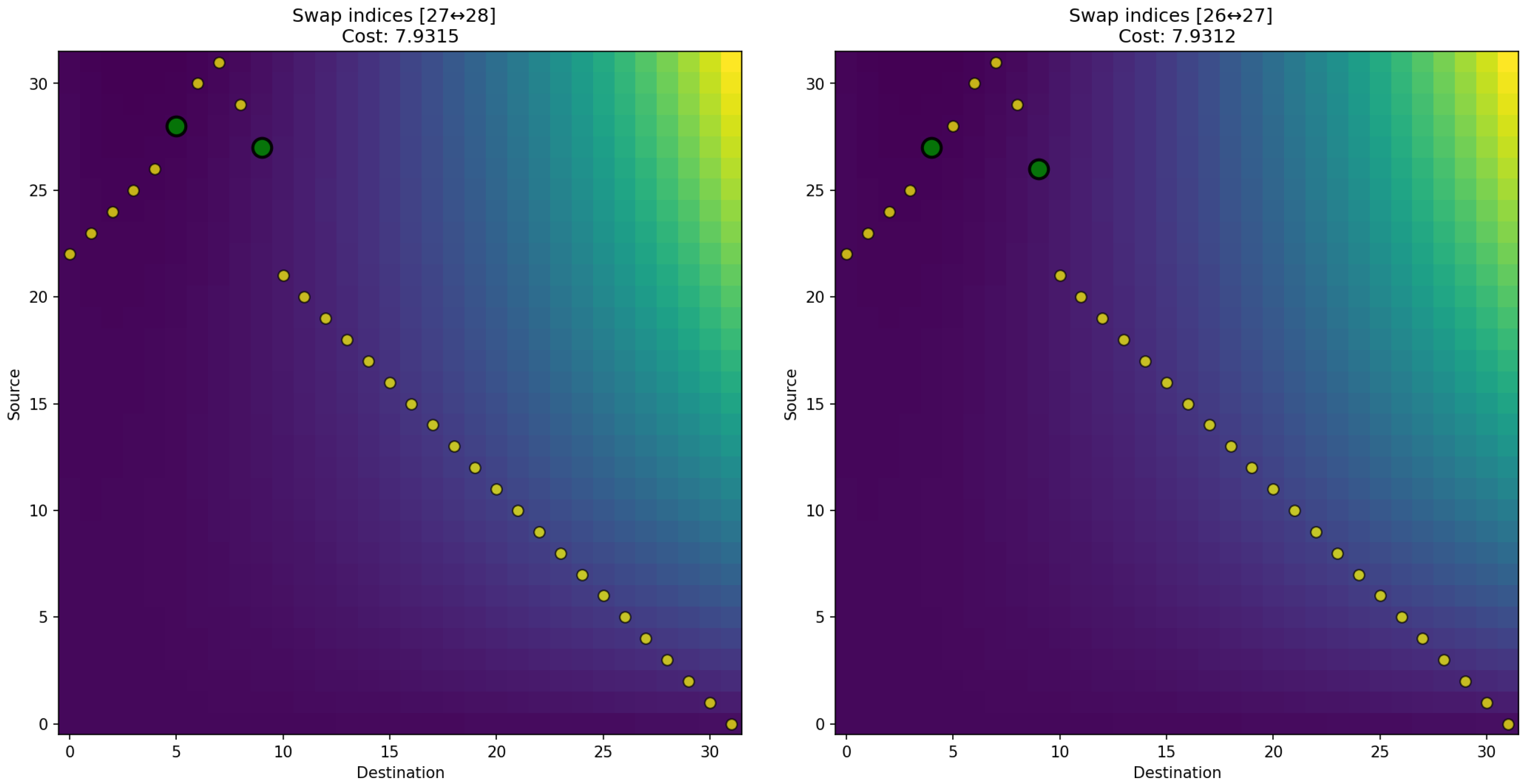
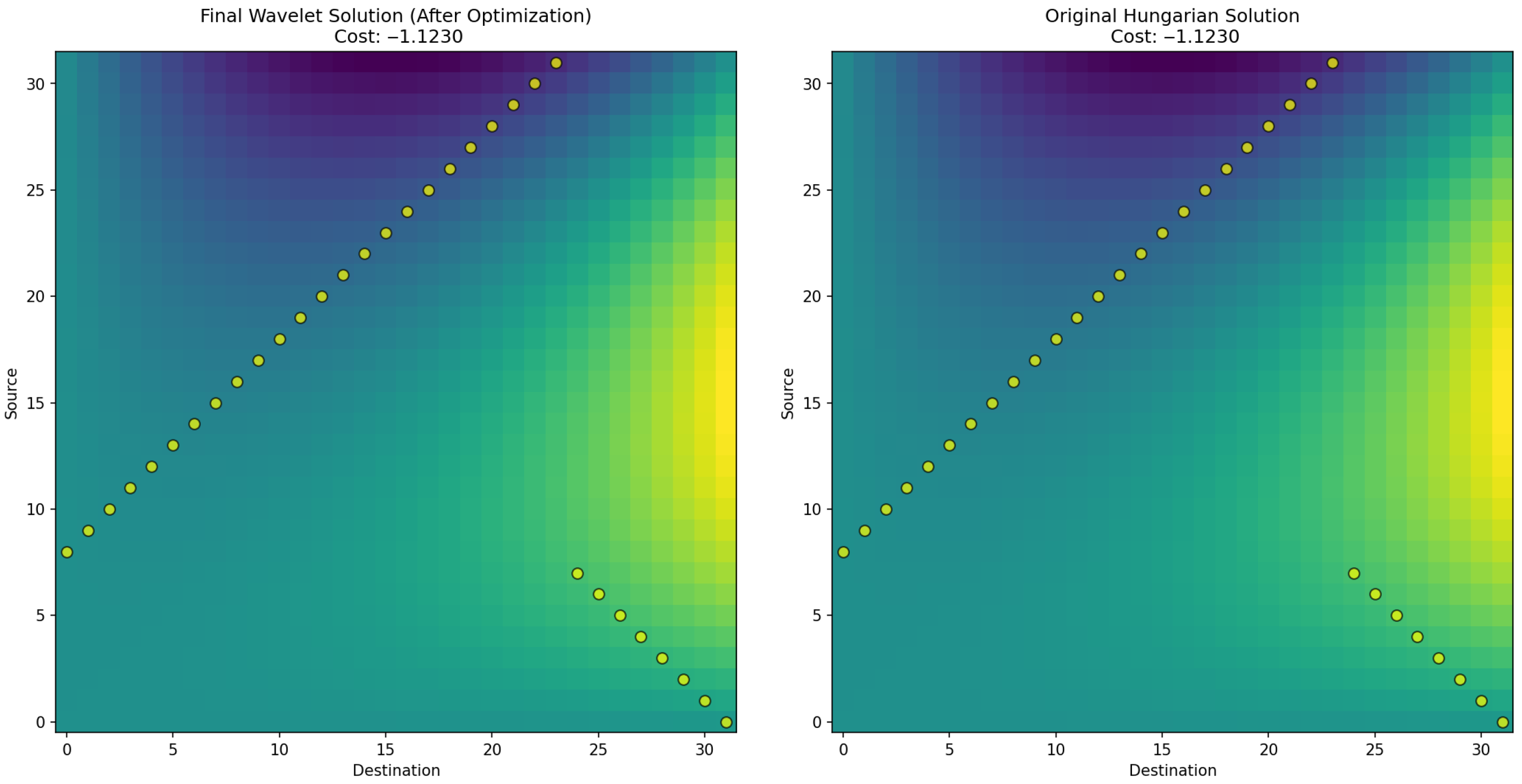
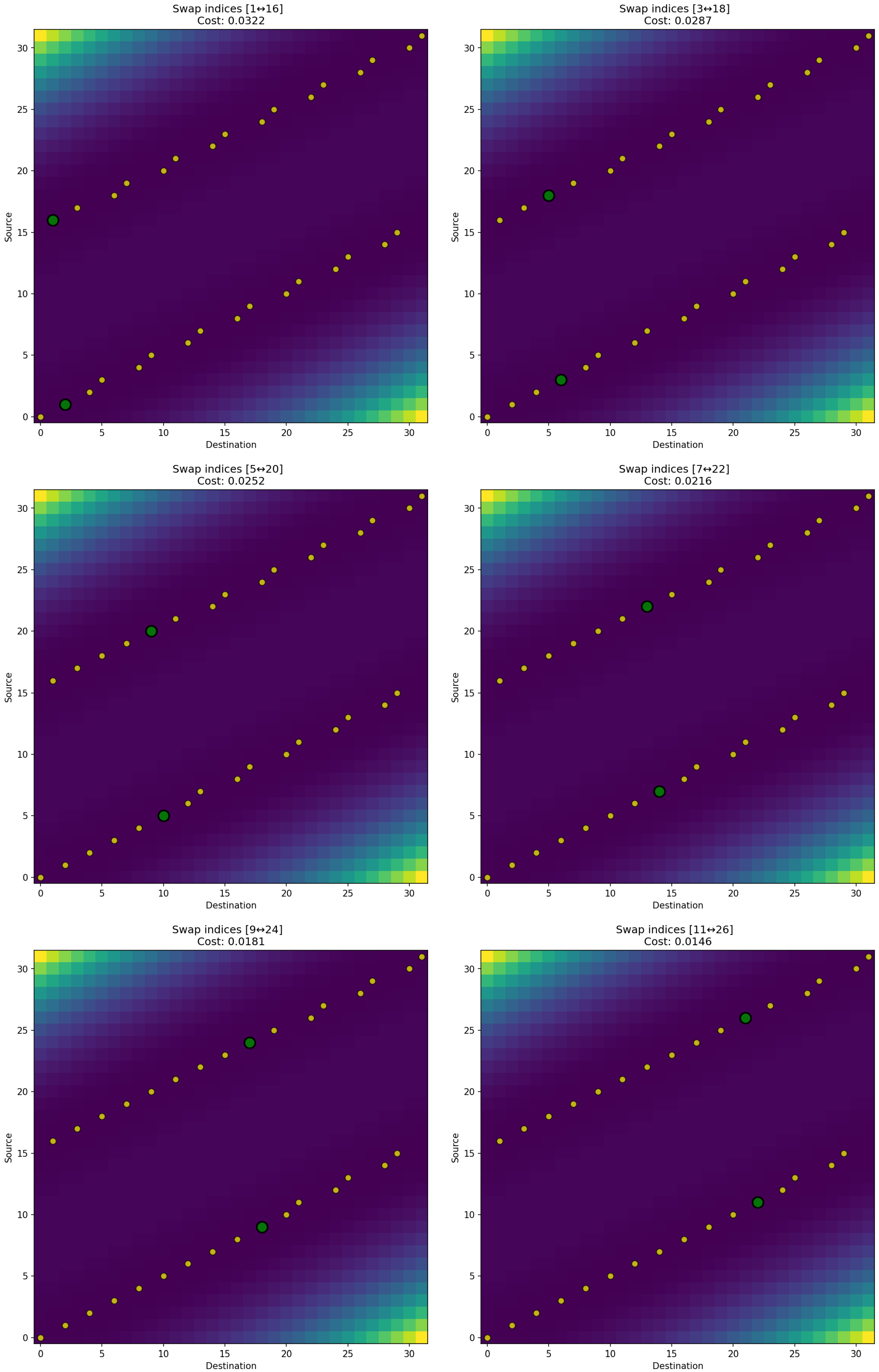
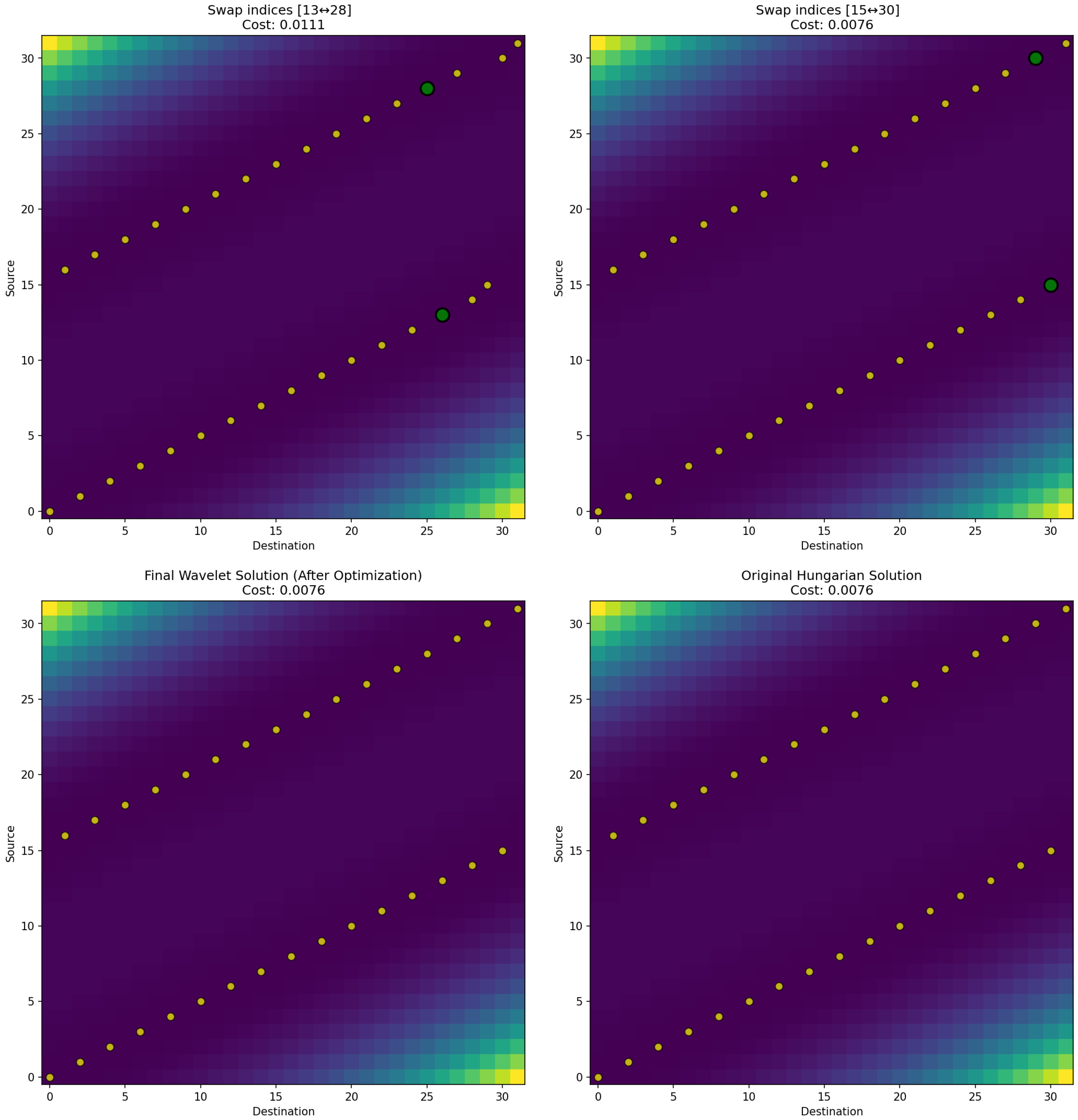
Below, we implement the automaton defined in (11), as illustrated in Figure 8:

Description of Figure 8:

• The upper figures illustrate the movements performed by the tuning automaton when the initial state is given by the right-hand panel of Figure 7. The green dots indicate the positions at which the automaton performed local optimizations. For clarity, steps in which no changes occurred are omitted.
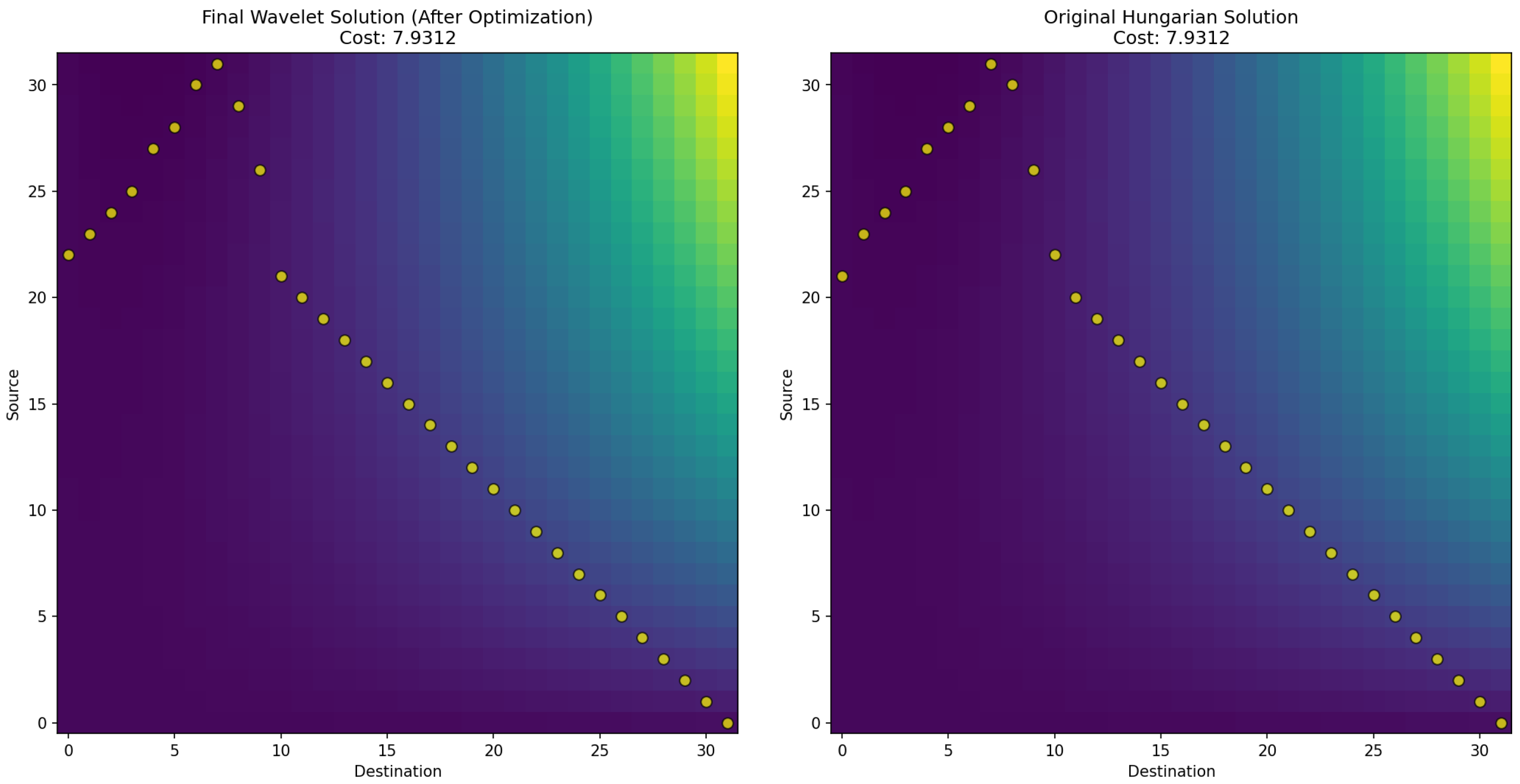
• The lower-left figure represents the final solution obtained by our procedure, which consists of applying the wavelet transform, solving the transportation problem with a $16\times 16$ cost matrix (level 4), extending the solution, and subsequently applying the automaton (level 5).
• The lower-right figure shows the solution obtained by directly solving the transportation problem with a $32\times 32$ cost matrix (level 5), as described in [12]. The solution obtained by our algorithm and the one obtained by directly applying the Hungarian algorithm are not identical; however, both produce the same minimum value, and therefore they can be considered equivalent solutions.
• In the numerical experiments presented in this work, the proposed automaton consistently converged to an optimal assignment. However, a complete theoretical characterization of the convergence properties of the method, including the precise conditions under which the optimal solution is unique, remains an open question. Determining such conditions and establishing formal convergence guarantees constitutes an interesting direction for future research.

5.2. Example 2

In this example, we consider the cost function $x^{2}y-x{y}^2$. The discretized function at level $j=5$ is shown in the following Figure 9:

The feasible ${\mu }_5$ solution at this level, according to [12], is shown in the following Figure 10:

On the other hand, by applying the wavelet transform to the discretization at level $j=5$, we obtain the decomposition in Figure 11, analogous to that shown in Figure 6.

By solving the transportation problem for the cost function given by the approximation at the lower level, we obtain the measure ${\mu }_4^{*}$. From this solution, we obtain the feasible solution ${\widehat{\mu }}_5^{*}$ (Figure 12) in a form analogous to that presented in Figure 7.

In this case, the measure ${\widehat{\mu }}_5$ constructed from ${\mu }_4^{*}$ coincides with the feasible measure ${\mu }_5$. Consequently, the automaton performs no modifications, as shown in Figure 13, which are analogous to those presented in the comparison carried out in the previous example.

5.3. Example 3

In this example, we consider the cost function ${(2y-x-1)}^2{(2y-x)}^2$. The discretized function at level $j=5$ is shown in the following Figure 14:

According to [12], the feasible measure ${\mu }_5$ at this level is illustrated in Figure 15.

By applying the wavelet transform to the discretization at level $j=5$, we obtain the decomposition in Figure 16, which is analogous to that shown in Figure 6.

The solution of the transportation problem corresponding to the cost function given by the lower-level approximation produces the measure ${\mu }_4$. From this result, we obtain a feasible solution ${\widehat{\mu }}_5$ (Figure 17), presented in a form analogous to that depicted in Figure 7.

Figure 18 illustrates both the changes produced by the implementation of the automaton on the feasible measure $\widehat{\mu }\ast 5$, resulting in the feasible measure $\mu \ast 5$, and the sequence of candidate solutions generated by the tuning automaton after applying the scaling procedure. The process begins with the approximation obtained after scaling and performing an initial adjustment, and each subsequent image corresponds to a new approximation produced while evaluating possible swaps. The penultimate image represents the final solution obtained by the automaton, whereas the last image shows the optimal solution computed using the Hungarian algorithm for comparison.

6. Conclusions

An important part of this work was the introduction of an automaton on the permutation group, which proved to be a useful tool to improve feasible solutions to the transportation problem associated with the MK problem. This represents a significant contribution to automata theory applied to optimization problems.

In all examples of transportation problems (assignment problem) associated with classic Monge–Kantorovich problems with a continuous cost function, these problems have the number of agents $2^j$. Therefore, solving this type of problem with the Hungarian algorithm has a computational cost of $O\left(2^{3j}\right)$.

Our methodology for solving the resulting transportation problems consists of the following steps:

1.

Apply the wavelet transform to a cost matrix of size $2^j\times 2^j$, which has a computational cost of $O\left(2^{2j}\right)$.

2.

Solve the transportation problem (assignment problem) over the approximation coefficients of the wavelet transform. At this coarser resolution level the problem involves $2^{j-1}$ agents, which is simpler than the original assignment problem. This reduced assignment problem is solved using the Hungarian algorithm in order to obtain an optimal assignment for the smaller cost matrix.

3.

Extending the solution from level $j-1$ to level j has a computational cost of $O\left(2^j\right)$, since it is only a fixed number of steps for each element of an array of size $2^j$.

4.

The computational cost of the linear automaton over the size of the array $2^j$, which is $O\left(2^j\right)$.

Therefore, the computational cost of this methodology for solving the transportation problem associated with the MK problem is significantly lower than that of applying the Hungarian algorithm directly. Since steps 1, 3, and 4 of our algorithm are of order $O\left(2^{2j}\right)$, the main computational cost of the methodology is concentrated in step 2. In this work, this step is solved by applying the Hungarian algorithm to a reduced problem involving only half of the agents.

Although the order of the Hungarian algorithm for this reduced problem is $O\left(2^{3j-3}\right)=O\left(2^{3j}\right)$, which in the worst case has the same asymptotic order, in practice fewer operations are required. Furthermore, to solve the problem with $2^{j-1}$ agents, our algorithm can be applied again, reducing the problem to one with $2^{j-2}$ agents, and so on. The study of the limits and scope of these techniques constitutes a direction for future research.

Furthermore, this methodology produced results equivalent to those obtained with the Hungarian algorithm for transport problems associated with MK problems. To illustrate this, three examples were presented at the level $j=5$, clearly demonstrating that equivalent results are obtained.

In the transportation problems considered in this article, the cost matrices are obtained from discretizations of a continuous function, which provides a certain degree of local stability to the matrix coefficients. Future work will aim to explore the limits of this technique in settings where the cost matrix exhibits higher entropy.

In Figure 3, the process begins with a random initial solution, to which the automaton is directly applied in order to solve the problem under consideration. In this case, the automaton successfully finds the optimal solution at level 3. However, the application of the automaton at higher levels of resolution was not investigated. As a direction for future research, it would be of interest to analyze the scope and limitations of applying the automaton to more general assignment problems, particularly in cases where the cost matrix is not derived from the discretization of a continuous function.

In addition, the technique will be evaluated by applying a greater number of multiresolution levels to the cost function in order to analyze its performance and robustness.

The automaton-based refinement strategy proposed in this work could also be applied to the optimal partial transport problem. In that setting, only a portion of the total mass is transported, which introduces additional constraints in the assignment structure. The local adjustment mechanism of the automaton, which operates through sequential swaps of assignments, could be adapted to handle partial matching by allowing unassigned elements or slack variables to represent unused mass. Although such an extension would require modifications to the state representation and the evaluation rules of the automaton, the underlying idea of iterative local refinement remains applicable. Investigating this extension and analyzing its numerical behavior constitutes an interesting direction for future research.