
Attention Measurement of an Autism Spectrum Disorder User Using EEG Signals: A Case Study

 ,
,  , , , , , ,
  and
and 
Abstract
1. Introduction
2. Materials and Methods
- Step 1.
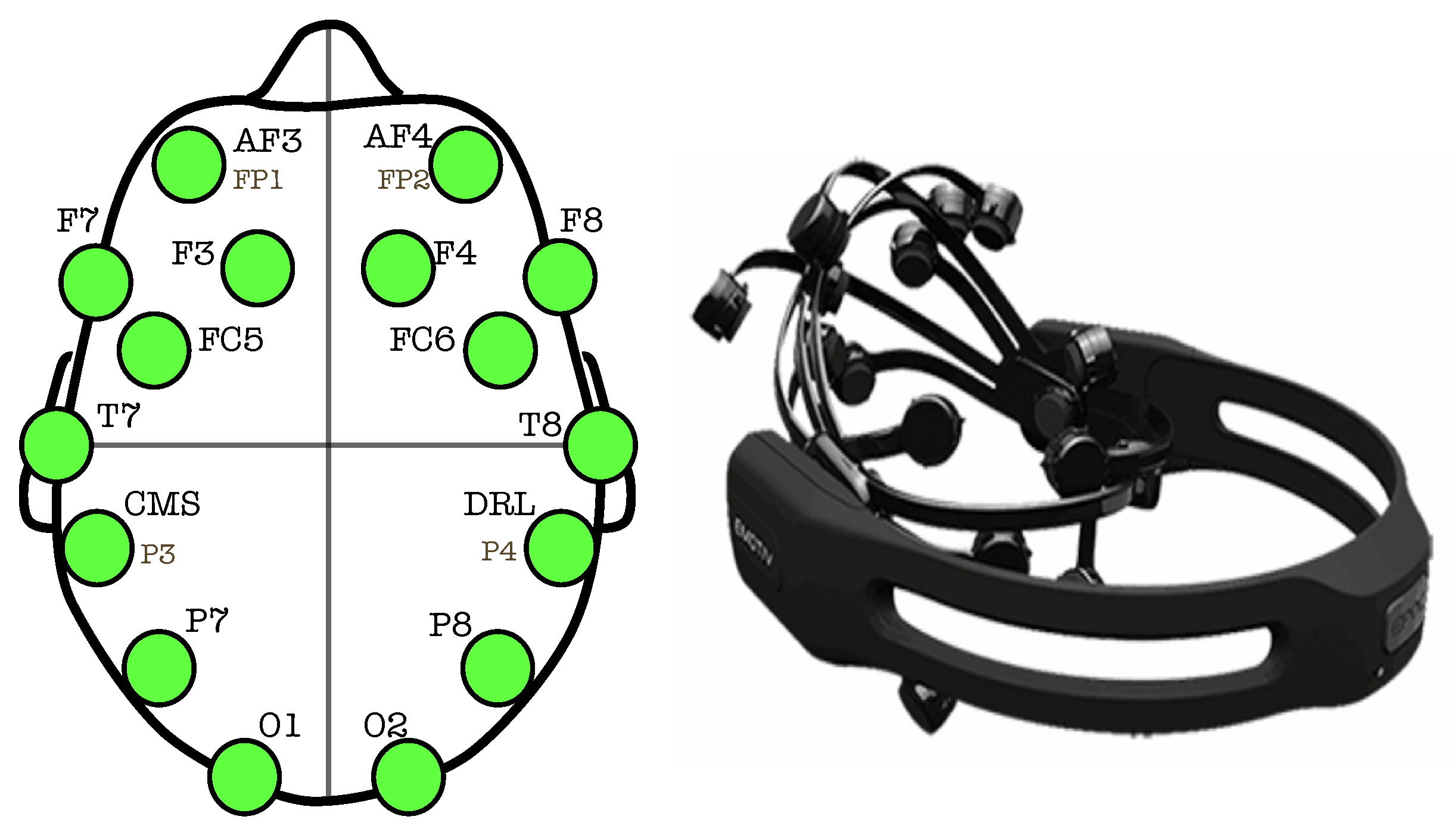
- Place the headset with the electrodes hydrated on the test subject.
- Step 2.
- Start the video recording and the EEG data acquisition.
- Step 3.
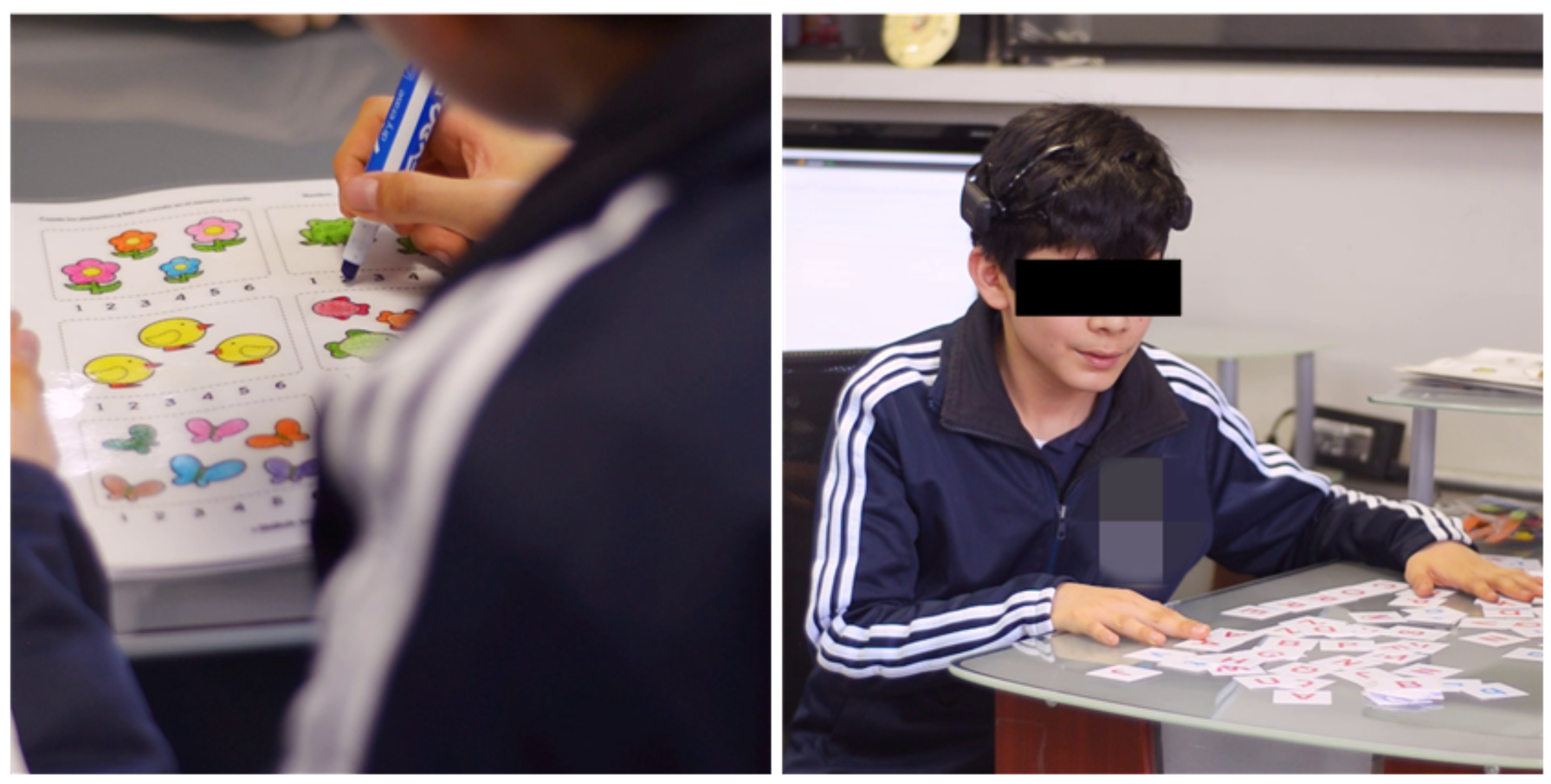
- Give the worksheet to the test subject and the instructions.
- Step 4.
- Let the test subject start the activity, and give him additional instructions if necessary, as in a regular school session.
- Step 5.
- When the activity is over, stop video recording and data acquisition.
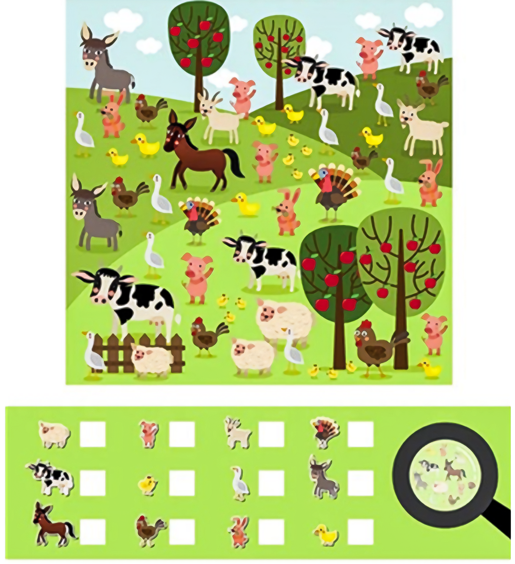
2.1. Activity Sheets
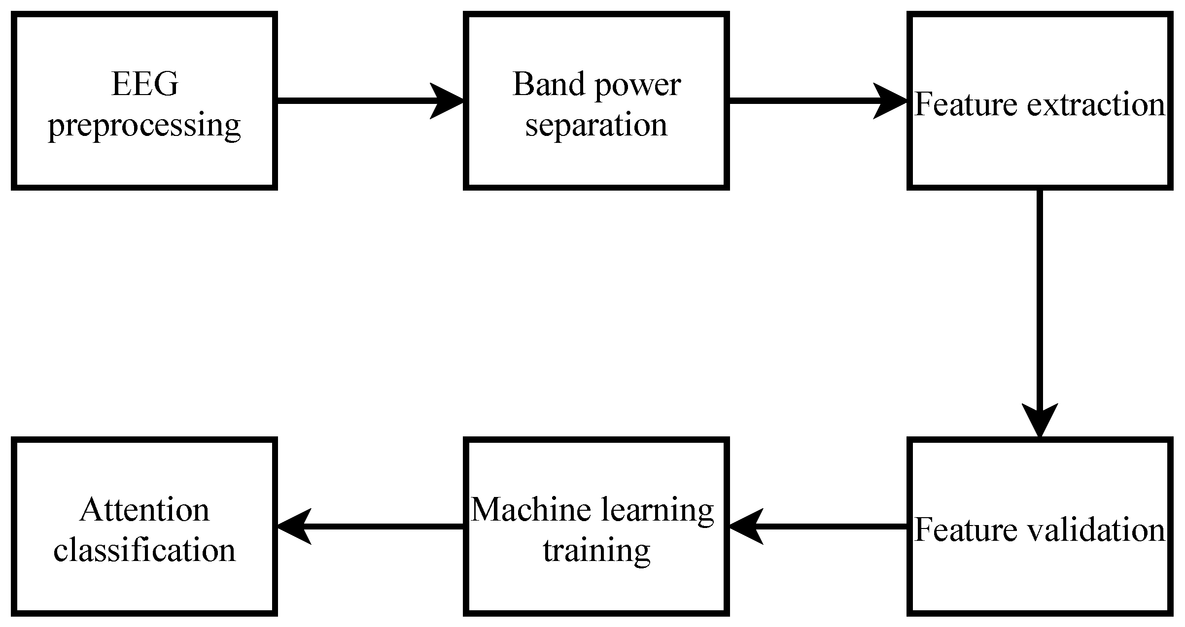
2.2. Signal Processing Procedure
2.2.1. Preprocessing of EEG Signal
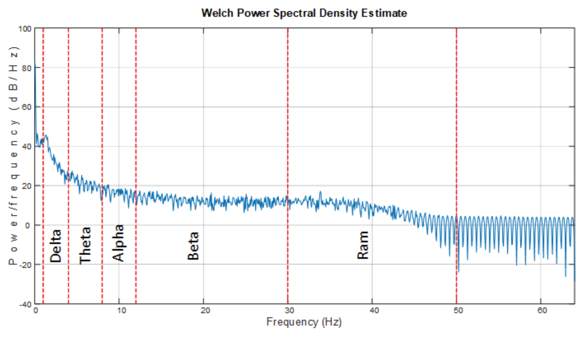
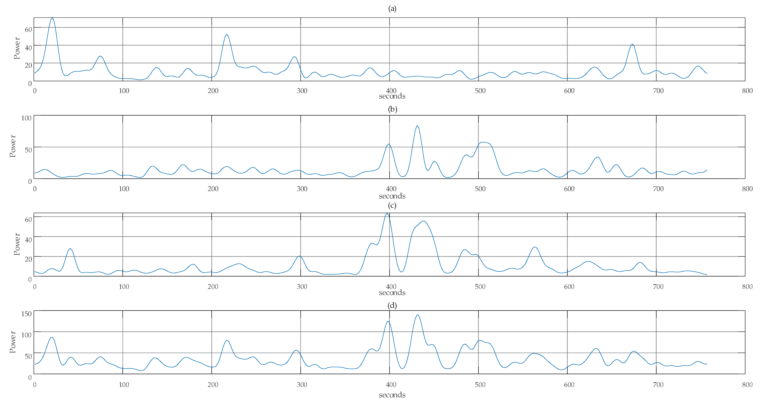
2.2.2. Band Power Separation
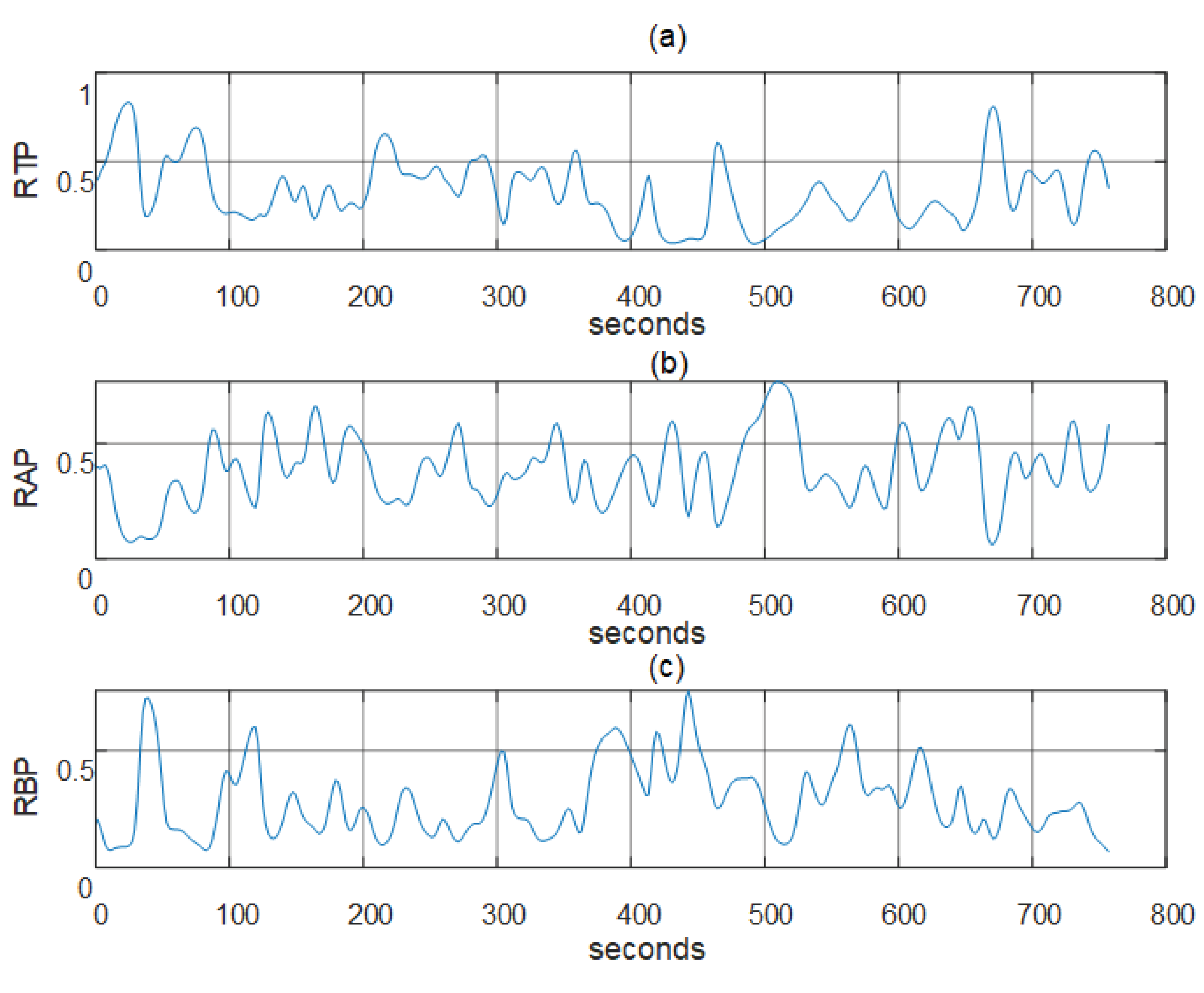
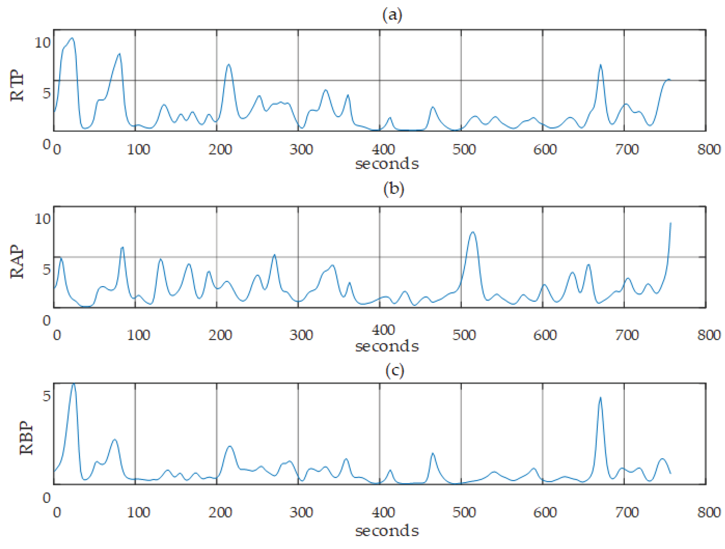
2.2.3. Feature Extraction

| Feature | Equation |
|---|---|
| Theta Relative Power | TRP |
| Alpha Relative Power | ARP |
| Beta Relative Power | BRP |
| Theta–Beta Ratio | TBR |
| Theta–Alpha Ratio | TAR |
| TBAR |
2.2.4. Dataset Preparation
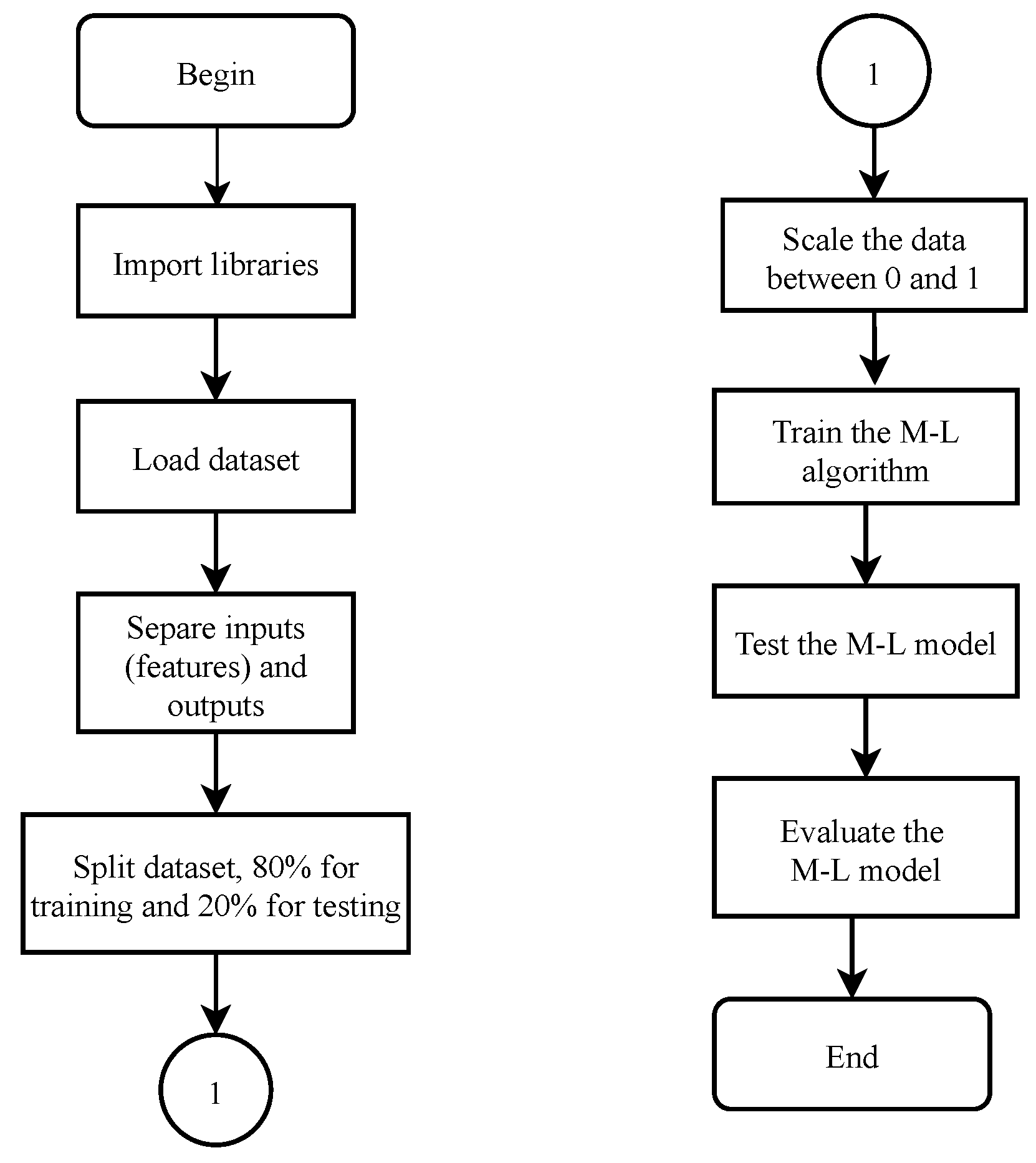
2.2.5. Machine Learning Algorithm Training
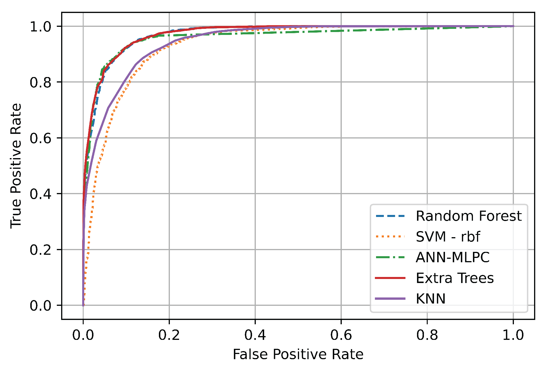
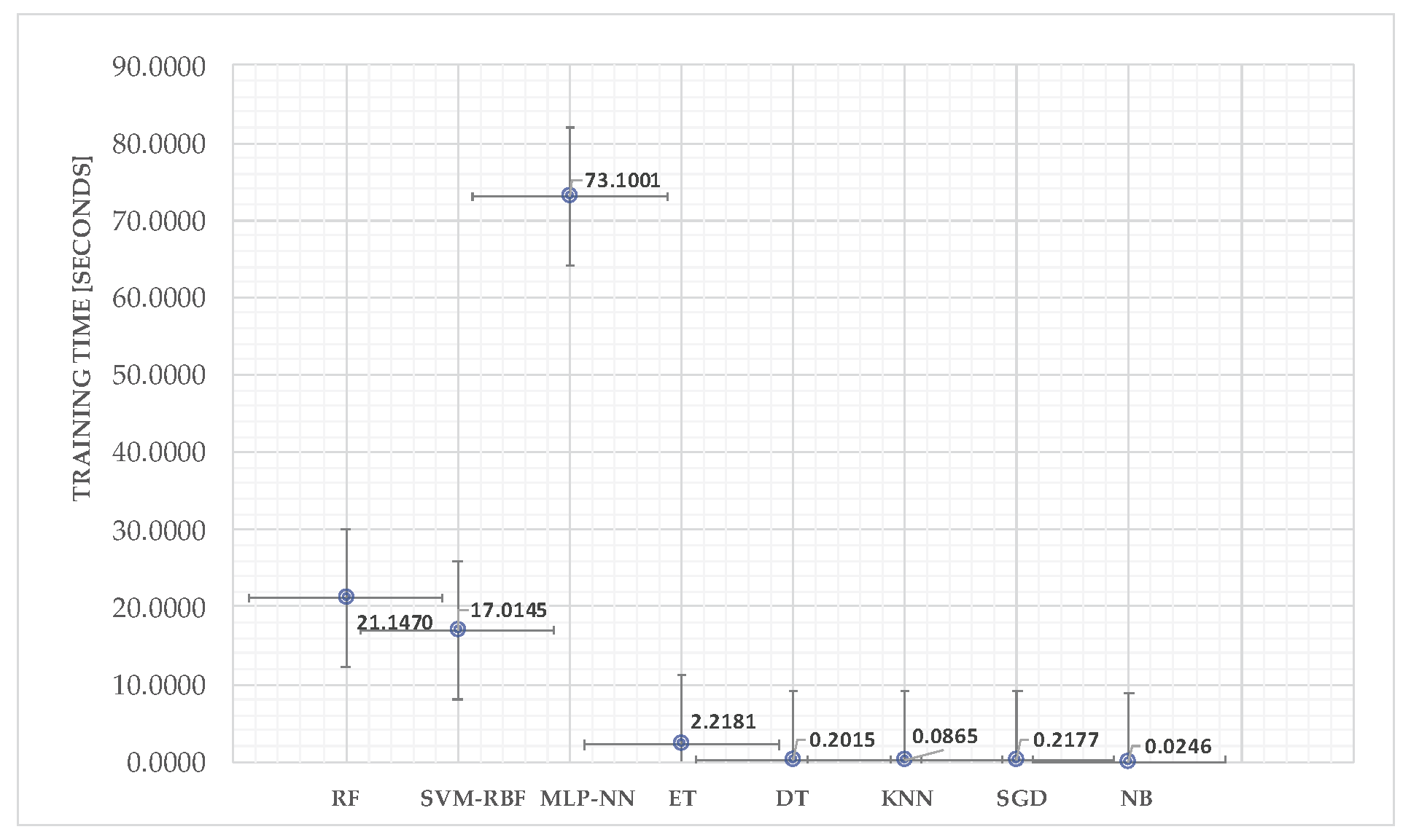
3. Results
4. Discussion
Limitations of the Study
5. Conclusions
Supplementary Materials
Author Contributions
Funding
Institutional Review Board Statement
Informed Consent Statement
Data Availability Statement
Acknowledgments
Conflicts of Interest
Abbreviations
| AI | Artificial Intelligence |
| ANFIS | Adaptive Neuro-Fuzzy Inference System |
| ASD | Autism Spectrum Disorder |
| BS | Breeding Swarm |
| CNN | Convolutional Neural Networks |
| DL | Deep Learning |
| fMRI | Functional Magnetic Resonance Imaging |
| GAN | Generative Adversarial Networks |
| LSTM | Long Short-Term Memories |
| MBP | Mindfulness-Based Program |
| ML | Machine Learning |
| MRI | Magnetic Resonance Imaging |
| PSD | Power Spectrum Density |
| RAP | Relative Alpha Power |
| RBP | Relative Beta Power |
| RNN | Recurrent Neural Network |
| RTP | Theta Relative Power |
| TAR | Theta–Alpha Ratio |
| TBR | Theta–Beta Ratio |
| TD | Typically Developed |
Appendix A. Comparison of the Proposed Method with the State of the Art
| Reference | Dataset | Data Source | Preprocessing | Method/Algorithm | Main Findings | Application |
|---|---|---|---|---|---|---|
| Ref. [20] | 12 ASD users and 12 typical children | EEG | N/A | Trial-averaged phase-locking value (PLV) approach and cubic support vector machine (SVM) | 95.8% Accuracy, 100% Sensitivity, and 92% Specificity | ASD Classification/Detection |
| Ref. [27] | 97 children aged from 3 to 6 | EEG, eye-tracking tests individually on own-race and other-race stranger faces stimuli. | Data were band-pass filtered between 0.5 and 45 Hz. To improve computing speed, EEG data were then down-sampled to 250 Hz. Power line noise in EEG was removed by a notch filter centered at 50 Hz. Artifacts in EEG were removed using an ICA approach (EEGLab). | SVM, minimum-redundancy-maximum-relevance (MRMR). | Classification Accuracy from combining two types of data reached a maximum of 85.44%, AUC 0.93, when 32 features were selected. | ASD Classification/Detection |
| Ref. [28] | 10 typically developing children (6 Male and 6 Female) and 10 autistic children (6 Male and 4 Female). | Natus Nihon Ohden MEB9000 version 05–81. | 22 channels, sampling frequency of 500 Hz and filtered with a low pass filter and a high pass filter at a frequency range of [0.53, 70] Hz. After filtering out the signal at a frequency range of 0.53 to 70 Hz, the ocular artifacts in the EEG signal were removed by thresholding. The threshold was set based on the average value of the amplitude of the eye blink signal. The eye blink signal was observed for 10 seconds with the eye open and eye close event. | ResNet50 | Average Accuracy of 81% | ASD Classification/Detection |
| Ref. [29] | N/A | EEG | Wavelet Transform, reduction of dimensionality, removal of irrelevant data. | K-Nearest Neighbour (KNN), A Correlation-based Feature Selection (CFS), Minimum Redundancy Maximum Relevance (MRMR) and the Information Gain (IG). | N/A | ASD Classification/Detection |
| Ref. [30] | Dataset from King Abdulaziz University (KAU) Hospital, Saudi Arabia. It is a public available dataset found in Sixteen subjects with twelve from ASD group (3 girls and 9 boys, age 6–20 years old) and four subjects from control group (all boys, 9–13 years old). | Spectrogram of EEG | Artifacts were removed from raw EEG data with re-referencing, filtering and normalization. Common average referencing (CAR) is used for re-referencing. IIR filter is used to low pass filter the signal at 40 Hz cut off frequency and finally the filtered signals from each electrode is normalized to the interval . signals are segmented into 3.5 second window frames for each subject to the dataset. Using Short-Time Fourier Transform (STFT) for each of the above segments, the spectrogram plot is generated in the last step and saved as image. | NB, LDA, RF, kNN, LR and SVM. Ten-fold cross validation. Three different CNN models. | The proposed DL based model achieves higher accuracy (99.15%) compared to the ML based model (95.25%) on an ASD EEG dataset and also outperforms existing methods. | ASD Classification/Detection |
| Ref. [31] | 5 Neurotypical and 8 ASD. | EEG | High-pass filtered at 1 Hz to remove slow trends and subsequently low-pass filtered at 50 Hz to remove line noise. The routine clinical bandwidth for EEG is from 0.5 to 50 Hz. | ML classifiers, namely support vector machine (SVM) and deep learning methods. | Multiclass two-layer LSTM RNN deep learning classifier is capable of identifying mental stress from ongoing EEG with an overall accuracy of 93.27%. | ASD Mental Stress |
| Ref. [32] | Study 1, 15 teenagers. Study 2, 20 subjects diagnosed with ASD and 20 subjects diagnosed with other neuropsychiatric disorders. | Artifact-free EEG data. | Raw EEG time-series were analyzed with a features extraction algorithm to extract 794 quantitative features (TSFRESH Python package). | TWIST, Sine-net ANN and Back Propagation ANN. | Sine-net ANN reached the best predictive capability in distinguishing autistic cases from typicals in study 1, Accuracy of 100%. Back Propagation ANN reached the best predictive capability in distinguishing autistic cases from subjects affected by other neuropsychiatric disorders in study 2 with an overall accuracy of 94.95%. | ASD Classification/Detection |
| Reference | Dataset | Data Source | Preprocessing | Method/Algorithm | Main Findings | Application |
|---|---|---|---|---|---|---|
| Ref. [33] | 122 subjects. | EEG to image converted | Spectrogram image generation model is presented using a combination of 1D_LBP and STFT. | Decision Tree (DT), Discriminant Analysis (DA), Logistic Regression (LR), SVM, K-Nearest Neighbor (kNN). | SVM classifier reached 96.44% Accuracy | ASD Classification/Detection |
| Ref. [38] | The disorder group comprises of 8 boys (10–16 years), and the normal group consists of 10 boys (9–16 years). Neuroimaging: ABIDE-I and ABIDE-II, which encompasses sMRI, rs-fMRI, and phenotypic data. ABIDE-I: a total of 1112 datasets, 539 individuals with ASD and 573 healthy individuals (ages 64–7). ABIDEII: 1114 datasets from 521 individuals with ASD and 593 healthy individuals (ages 5–64). | Neuroimaging, fMRI, MRI, EEG | Several preprocesing applied to all signals. | Supervised learning, unsupervised learning, and reinforcement learning (RL). | Presents challenges and performances of DL techniques | ASD Classification/Rehabilitation |
| Ref. [39] | MICCAI 2008, MICCAI 2016, ISBI 2015, and eHealth Lab. | MRI | Low level and high level preprocessing methods in MRI. | Most popular DL architectures for MS detection: convolutional neural networks (CNNs), Autoencoders (AEs), generative adversarial networks (GANs), and CNN-RNN models. | The inaccessibility of huge sMRI datasets belonging to a diverse population and lack of access to fMRI modalities are among the most important dataset-related challenges which are discussed in detail. Moreover, DL-related challenges include researchers’ lack of access to powerful hardware resources for MS diagnosis research. | Multiple Sclerosis Detection |
| Ref. [40] | Dataset of the Institute of Psychiatry and Neurology in Warsaw. | EEG | EEG signals were divided into 25 s time frames and then normalized by z-score or norm L2. | EEG signals Classification: support vector machine, k-nearest neighbors, Decision Tree, Naive Bayes, Random Forest, extremely randomized trees, and bagging. DL models: long short-term memories (LSTMs), one-dimensional convolutional networks (1D-CNNs), and 1D-CNN-LSTM. | CNN-LSTM model accuracy of 99.25%. | Schizophrenia/Diagnosis |
| Ref. [41] | Bonn University dataset with six classification combinations and the Freiburg dataset. | EEG | Tunable-Q wavelet transform (TQWT) for EEG signal decomposition. Feature extraction, 13 different fuzzy entropies calculated from TQWT. Six layers Autoencoder (AE) for dimensionality reduction. | Classification: Adaptive neuro-fuzzy inference system (ANFIS), and also its variants with grasshopper optimization algorithm (ANFIS-GOA), particle swarm optimization (ANFIS-PSO), and breeding swarm optimization (ANFIS-BS). | ANFIS-BS two classes classification Accuracy: 99.74%; an Accuracy of 99.46% in ternary classification on the Bonn dataset, and 99.28% on the Freiburg dataset. | Detection of epileptic seizures |
| Proposed method | 1 Subject, 33936 samples | EEG and BCI | Scaling, 2 seconds Band Power Separation. Features: TRP, ARP, BRP, TBR, TAR, and Theta/(alpha+beta). | Naive Bayes, Stochastic Gradient Descent, Decision trees, SVM, KNN, MLP-NN, RF, Extra trees. | (MLP-NN) with Accuracy 92.98%, Sensitivity 94.59%, F1 Score 93.04%, Specificity 91.55%, AUC of 0.9299, Cohen’s Kappa coefficient of 0.8597, Matthews correlation coefficient of 0.8602, and Hamming loss of 0.0701. | ASD Attention Classification |
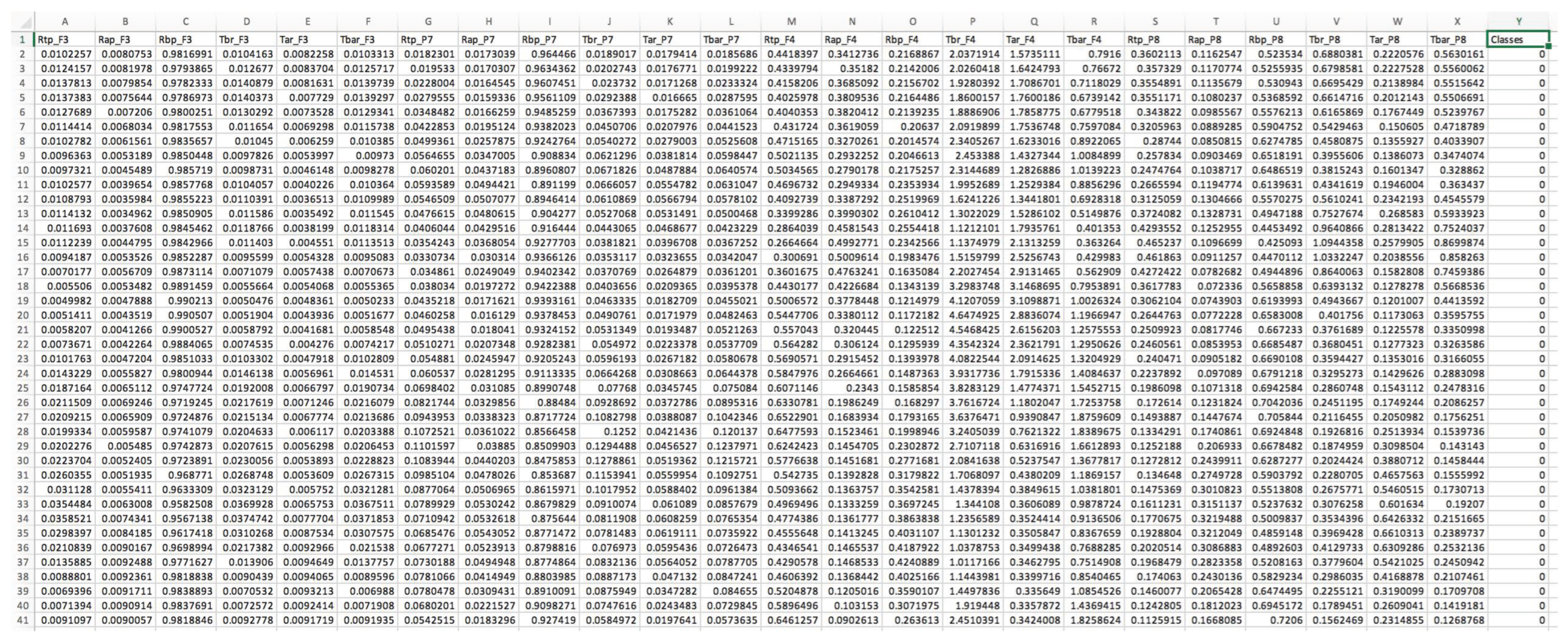
Appendix B. Fragment of the Dataset Created for This Study

References
- Howe, T.R.; Trotter, J.S.; Davis, A.S.; Schofield, J.W.; Allen, L.; Millians, M.; Bolt, N. Attention Span; Springer: New York, NY, USA, 2011. [Google Scholar] [CrossRef]
- American Psychiatric Association. Diagnostic and Statistical Manual of Mental Disorders: DSM-5, 5th ed.; American Psychiatric Publishing: Washington, DC, USA, 2013; p. 947. [Google Scholar]
- Goqvkqpcn, E.; Ogpvcn, E. Autism Spectrum Disorder. Nat. Rev. Dis. Prim. 2020, 6, 6. [Google Scholar] [CrossRef]
- Ishizaki, Y.; Higuchi, T.; Yanagimoto, Y.; Kobayashi, H.; Noritake, A.; Nakamura, K.; Kaneko, K. Eye gaze differences in school scenes between preschool children and adolescents with high-functioning autism spectrum disorder and those with typical development. BioPsychoSoc. Med. 2021, 15, 2. [Google Scholar] [CrossRef] [PubMed]
- Egger, H.L.; Dawson, G.; Hashemi, J.; Carpenter, K.L.H.; Espinosa, S.; Campbell, K.; Brotkin, S.; Schaich-Borg, J.; Qiu, Q.; Tepper, M.; et al. Automatic emotion and attention analysis of young children at home: A ResearchKit autism feasibility study. NPJ Digit. Med. 2018, 1, 20. [Google Scholar] [CrossRef] [PubMed]
- Son, J.; Ai, L.; Lim, R.; Xu, T.; Colcombe, S.; Franco, A.R.; Cloud, J.; LaConte, S.; Lisinski, J.; Klein, A.; et al. Evaluating fMRI-Based Estimation of Eye Gaze During Naturalistic Viewing. Cereb. Cortex 2020, 30, 1171–1184. [Google Scholar] [CrossRef]
- Lawrence, S.J.D.; Formisano, E.; Muckli, L.; De Lange, F.P. Laminar fMRI: Applications for cognitive neuroscience. NeuroImage 2019, 197, 785–791. [Google Scholar] [CrossRef]
- Ridderinkhof, A.; De Bruin, E.I.; Driesschen, S.v.d.; Bögels, S.M. Attention in Children with Autism Spectrum Disorder and the Effects of a Mindfulness-Based Program. J. Atten. Disord. 2018, 24, 681–692. [Google Scholar] [CrossRef] [PubMed]
- Ababkova, M.; Leontieva, V.; Trostinskaya, I.; Pokrovskaia, N. Biofeedback as a cognitive research technique for enhancing learning process. IOP Conf. Ser. Mater. Sci. Eng. 2020, 940, 012127. [Google Scholar] [CrossRef]
- Lau-Zhu, A.; Lau, M.; McLoughlin, G. Mobile EEG in research on neurodevelopmental disorders: Opportunities and challenges. Dev. Cogn. Neurosci. 2019, 36, 100635. [Google Scholar] [CrossRef]
- Mehmood, F.; Ayaz, Y.; Ali, S.; Amadeu, R.D.C.; Sadia, H. Dominance in Visual Space of ASD Children Using Multi-Robot Joint Attention Integrated Distributed Imitation System. IEEE Access 2019, 7, 168815–168827. [Google Scholar] [CrossRef]
- Wang, H.; Song, Q.; Ma, T.; Cao, H.; Sun, Y. Study on Brain-Computer Interface Based on Mental Tasks. In Proceedings of the 5th Annual IEEE International Conference on Cyber Technology in Automation, Control and Intelligent Systems, Shenyang, China, 8–12 June 2015; pp. 841–845. [Google Scholar] [CrossRef]
- Ismail, L.E.; Karwowski, W. Applications of EEG indices for the quantification of human cognitive performance: A systematic review and bibliometric analysis. PLoS ONE 2020, 15, e0242857. [Google Scholar] [CrossRef] [PubMed]
- Niemarkt, H.J.; Jennekens, W.; Maartens, I.A.; Wassenberg, T.; van Aken, M.; Katgert, T.; Kramer, B.W.; Gavilanes, A.W.; Zimmermann, L.J.; Bambang Oetomo, S.; et al. Multi-channel amplitude-integrated EEG characteristics in preterm infants with a normal neurodevelopment at two years of corrected age. Early Hum. Dev. 2012, 88, 209–216. [Google Scholar] [CrossRef] [PubMed]
- Micoulaud-Franchi, J.A.; Batail, J.M.; Fovet, T.; Philip, P.; Cermolacce, M.; Jaumard-Hakoun, A.; Vialatte, F. Towards a Pragmatic Approach to a Psychophysiological Unit of Analysis for Mental and Brain Disorders: An EEG-Copeia for Neurofeedback. Appl. Psychophysiol. Biofeedback 2019, 44, 151–172. [Google Scholar] [CrossRef] [PubMed]
- Singh, M.I.; Singh, M. Development of low-cost event marker for EEG-based emotion recognition. Trans. Inst. Meas. Control 2017, 39, 642–652. [Google Scholar] [CrossRef]
- Yang, L.; Wilke, C.; Brinkmann, B.; Worrell, G.A.; He, B. Dynamic imaging of ictal oscillations using non-invasive high-resolution EEG. Neuroimage 2011, 56, 1908–1917. [Google Scholar] [CrossRef]
- Ismail, L.I.; Shamsudin, S.; Yussof, H.; Hanapiah, F.A.; Zahari, N.I. Estimation of concentration by eye contact measurement in Robot-based Intervention Program with autistic children. Procedia Eng. 2012, 41, 1548–1552. [Google Scholar] [CrossRef][Green Version]
- Zhang, S.; Chen, D.; Tang, Y.; Zhang, L. Children ASD Evaluation Through Joint Analysis of EEG and Eye-Tracking Recordings with Graph Convolution Network. Front. Hum. Neurosci. 2021, 15, 651349. [Google Scholar] [CrossRef] [PubMed]
- Alotaibi, N.; Maharatna, K. Classification of Autism Spectrum Disorder from EEG-Based Functional Brain Connectivity Analysis. Neural Comput. 2021, 33, 1914–1941. [Google Scholar] [CrossRef] [PubMed]
- Cerrada, M.; Trujillo, L.; Hernández, D.E.; Correa Zevallos, H.A.; Macancela, J.C.; Cabrera, D.; Vinicio Sánchez, R. AutoML for Feature Selection and Model Tuning Applied to Fault Severity Diagnosis in Spur Gearboxes. Math. Comput. Appl. 2022, 27, 6. [Google Scholar] [CrossRef]
- Enríquez Zárate, J.; Gómez López, M.d.l.A.; Carmona Troyo, J.A.; Trujillo, L. Analysis and Detection of Erosion in Wind Turbine Blades. Math. Comput. Appl. 2022, 27, 5. [Google Scholar] [CrossRef]
- Janiesch, C.; Zschech, P.; Heinrich, K. Machine learning and deep learning. Electron. Mark. 2021, 31, 685–695. [Google Scholar] [CrossRef]
- Fong-Mata, M.; García-Guerrero, E.; Mejia-Medina, D.; López-Bonilla, O.; Villarreal-Gomez, L.; Zamora-Arellano, F.; López-Mancilla, D.; Inzunza-González, E. An Artificial Neural Network Approach and a Data Augmentation Algorithm to Systematize the Diagnosis of Deep-Vein Thrombosis by Using Wells’ Criteria. Electronics 2020, 9, 1810. [Google Scholar] [CrossRef]
- Choi, R.Y.; Coyner, A.S.; Kalpathy-Cramer, J.; Chiang, M.F.; Campbell, J.P. Introduction to Machine Learning, Neural Networks, and Deep Learning. Transl. Vis. Sci. Technol. 2020, 9, 14. [Google Scholar] [CrossRef]
- Navarro-Espinoza, A.; López-Bonilla, O.R.; García-Guerrero, E.E.; Tlelo-Cuautle, E.; López-Mancilla, D.; Hernández-Mejía, C.; Inzunza-González, E. Traffic Flow Prediction for Smart Traffic Lights Using Machine Learning Algorithms. Technologies 2022, 10, 5. [Google Scholar] [CrossRef]
- Kang, J.; Han, X.; Song, J.; Niu, Z.; Li, X. The identification of children with autism spectrum disorder by SVM approach on EEG and eye-tracking data. Comput. Biol. Med. 2020, 120, 103722. [Google Scholar] [CrossRef] [PubMed]
- Radhakrishnan, M.; Ramamurthy, K.; Choudhury, K.K.; Won, D.; Manoharan, T.A. Performance analysis of deep learning models for detection of Autism Spectrum Disorder from EEG signals. Trait. Signal 2021, 38, 853–863. [Google Scholar] [CrossRef]
- Thirumal, S.; Thangakumar, J. Investigation of Statistical Feature Selection Techniques for Autism Classification Using EEG Signals. J. Adv. Res. Dyn. Control Syst. 2020, 12, 1254–1263. [Google Scholar] [CrossRef]
- Tawhid, M.N.A.; Siuly, S.; Wang, H.; Whittaker, F.; Wang, K.; Zhang, Y. A spectrogram image based intelligent technique for automatic detection of autism spectrum disorder from EEG. PLoS ONE 2021, 16, e0253094. [Google Scholar] [CrossRef]
- Sundaresan, A.; Penchina, B.; Cheong, S.; Grace, V.; Valero-Cabré, A.; Martel, A. Evaluating deep learning EEG-based mental stress classification in adolescents with autism for breathing entrainment BCI. Brain Inform. 2021, 8. [Google Scholar] [CrossRef]
- Grossi, E.; Valbusa, G.; Buscema, M. Detection of an Autism EEG Signature From Only Two EEG Channels Through Features Extraction and Advanced Machine Learning Analysis. Clin. EEG Neurosci. 2021, 52, 330–337. [Google Scholar] [CrossRef] [PubMed]
- Baygin, M.; Dogan, S.; Tuncer, T.; Datta Barua, P.; Faust, O.; Arunkumar, N.; Abdulhay, E.W.; Emma Palmer, E.; Rajendra Acharya, U. Automated ASD detection using hybrid deep lightweight features extracted from EEG signals. Comput. Biol. Med. 2021, 134, 104548. [Google Scholar] [CrossRef] [PubMed]
- Hagendorff, T. Linking Human And Machine Behavior: A New Approach to Evaluate Training Data Quality for Beneficial Machine Learning. Minds Mach. 2021, 31, 563–593. [Google Scholar] [CrossRef] [PubMed]
- Swatzyna, R.J.; Boutros, N.N.; Genovese, A.C.; MacInerney, E.K.; Roark, A.J.; Kozlowski, G.P. Electroencephalogram (EEG) for children with autism spectrum disorder: Evidential considerations for routine screening. Eur. Child Adolesc. Psychiatry 2019, 28, 615–624. [Google Scholar] [CrossRef] [PubMed]
- Kurgansky, A.V.; Machinskaya, R. Bilateral frontal theta-waves in EEG of 7–8-year-old children with learning difficulties: Qualitative and quantitative analysis. Hum. Physiol. 2012, 38, 255–263. [Google Scholar] [CrossRef]
- Machinskaya, R.; Semenova, O.A.; Absatova, K.A.; Sugrobova, G.A. Neurophysiological factors associated with cognitive deficits in children with ADHD symptoms: EEG and neuropsychological analysis. Psychol. Neurosci. 2014, 7, 461–473. [Google Scholar] [CrossRef]
- Khodatars, M.; Shoeibi, A.; Sadeghi, D.; Ghaasemi, N.; Jafari, M.; Moridian, P.; Khadem, A.; Alizadehsani, R.; Zare, A.; Kong, Y.; et al. Deep learning for neuroimaging-based diagnosis and rehabilitation of Autism Spectrum Disorder: A review. Comput. Biol. Med. 2021, 139, 104949. [Google Scholar] [CrossRef]
- Shoeibi, A.; Khodatars, M.; Jafari, M.; Moridian, P.; Rezaei, M.; Alizadehsani, R.; Khozeimeh, F.; Gorriz, J.M.; Heras, J.; Panahiazar, M.; et al. Applications of deep learning techniques for automated multiple sclerosis detection using magnetic resonance imaging: A review. Comput. Biol. Med. 2021, 136, 104697. [Google Scholar] [CrossRef] [PubMed]
- Shoeibi, A.; Sadeghi, D.; Moridian, P.; Ghassemi, N.; Heras, J.; Alizadehsani, R.; Khadem, A.; Kong, Y.; Nahavandi, S.; Zhang, Y.D.; et al. Automatic Diagnosis of Schizophrenia in EEG Signals Using CNN-LSTM Models. Front. Neuroinform. 2021, 15. [Google Scholar] [CrossRef]
- Shoeibi, A.; Ghassemi, N.; Khodatars, M.; Moridian, P.; Alizadehsani, R.; Zare, A.; Khosravi, A.; Subasi, A.; Rajendra Acharya, U.; Gorriz, J.M. Detection of epileptic seizures on EEG signals using ANFIS classifier, autoencoders and fuzzy entropies. Biomed. Signal Process. Control 2022, 73, 103417. [Google Scholar] [CrossRef]
- Khng, K.H.; Mane, R. Beyond BCI—Validating a wireless, consumer-grade EEG headset against a medical-grade system for evaluating EEG effects of a test anxiety intervention in school. Adv. Eng. Inform. 2020, 45, 101106. [Google Scholar] [CrossRef]
- Fouad, I. A robust and reliable online P300 based BCI system using Emotiv EPOC Headset. J. Med. Eng. Technol. 2021, 45, 94–114. [Google Scholar] [CrossRef]
- Dubrovinskaya, N.; Machinska, R.; Kulakovsky, Y. Brain Organization of Selective Tasks Preceding Attention: Ontogenetic Aspects. In Complex Brain Functions: Conceptual Advances in Russian Neurocience; CRC Press: Boca Raton, FL, USA, 2000; Volume 1, pp. 169–180. [Google Scholar] [CrossRef]
- Dubrovinskaya, N.V.; Machinskaya, R.I. Reactivity of Teta and Alpha EEG Frequency Bands in Voluntary Attention in Junior Schoolchildren. Hum. Physiol. 2002, 28, 522–527. [Google Scholar] [CrossRef]
- Emotiv, I. Data Sample Object. Cortex API. Available online: https://emotiv.gitbook.io/cortex-api/data-subscription/data-sample-object (accessed on 29 December 2021).
- Emotiv, I. Frequency Bands Emotiv PRO v3.0. Available online: https://emotiv.gitbook.io/emotivpro-v3/ (accessed on 29 December 2021).
- Fahimi, F.; Guan, C.; Wooi, B.G.; Kai Keng, A.; Choon, G.L.; Tih, S.L. Personalized features for attention detection in children with Attention Deficit Hyperactivity Disorder. In Proceedings of the Annual International Conference of the IEEE Engineering in Medicine and Biology Society, EMBS, Jeju, Korea, 11–15 July 2017; pp. 414–417. [Google Scholar] [CrossRef]
- Pedregosa, F.; Varoquaux, G.; Gramfort, A.; Michel, V.; Thirion, B.; Grisel, O.; Blondel, M.; Prettenhofer, P.; Weiss, R.; Dubourg, V.; et al. Scikit-Learn: Machine Learning in Python. 2011. Available online: https://scikit-learn.org (accessed on 29 December 2021).
- Matthews, B.W. Comparison of the predicted and observed secondary structure of T4 phage lysozyme. Biochim. Biophys. Acta (BBA)—Protein Struct. 1975, 405, 442–451. [Google Scholar] [CrossRef]
- Ein Shoka, A.A.; Alkinani, M.H.; El-Sherbeny, A.S.; El-Sayed, A.; Dessouky, M.M. Automated seizure diagnosis system based on feature extraction and channel selection using EEG signals. Brain Inform. 2021, 8, 1. [Google Scholar] [CrossRef] [PubMed]
- Misiunas, A.V.M.; Meskauskas, T.; Samaitiene, R. Machine Learning Based EEG Classification by Diagnosis: Approach to EEG Morphological Feature Extraction. AIP Conf. Proc. 2019, 2164, 080005. [Google Scholar] [CrossRef]
- Boroujeni, Y.K.; Rastegari, A.A.; Khodadadi, H. Diagnosis of attention deficit hyperactivity disorder using non-linear analysis of the EEG signal. IET Syst. Biol. 2019, 13, 260–266. [Google Scholar] [CrossRef] [PubMed]


| Machine-Learning Algorithm | ||||||||
|---|---|---|---|---|---|---|---|---|
| Scoring Parameters | Naive Bayes | SGD | Decision Trees | (SVM)-RBF | KNN | MLP-NN | Random Forest (RF) | Extra Trees |
| True positive | 1984 | 2720 | 2967 | 2874 | 2892 | 3126 | 3039 | 3013 |
| True negative | 3194 | 3131 | 2937 | 3195 | 3196 | 3186 | 3268 | 3280 |
| False positive | 1436 | 700 | 453 | 546 | 528 | 294 | 381 | 407 |
| False negative | 174 | 237 | 431 | 173 | 172 | 182 | 100 | 88 |
| Accuracy | 0.7628 | 0.8619 | 0.8697 | 0.8940 | 0.8968 | 0.9298 | 0.9291 | 0.9270 |
| F1 Score | 0.7986 | 0.8698 | 0.8691 | 0.8988 | 0.9012 | 0.9304 | 0.9314 | 0.9278 |
| Specificity/Precision | 0.6898 | 0.8172 | 0.8663 | 0.8540 | 0.8582 | 0.9155 | 0.8955 | 0.8896 |
| Sensitivity/Recall | 0.9483 | 0.9296 | 0.8720 | 0.9486 | 0.9489 | 0.9459 | 0.9703 | 0.9738 |
| Performance Metrics | ||||
|---|---|---|---|---|
| Machine Learning Algorithm | AUC | Cohen’s KappaCoefficient | Hamming Loss | MatthewsCorrelation Coefficient |
| Naive Bayes | 0.7642 | 0.5269 | 0.2371 | 0.5674 |
| Stochastic Gradient Descent | 0.8624 | 0.7241 | 0.1380 | 0.7310 |
| Decision Trees | 0.8697 | 0.7395 | 0.1302 | 0.7395 |
| Support Vector Machine (SVM)-RBF | 0.8944 | 0.7883 | 0.1059 | 0.7931 |
| KNN | 0.8972 | 0.7939 | 0.1031 | 0.7983 |
| Extra Trees | 0.9274 | 0.8542 | 0.0729 | 0.8580 |
| MLP-NN | 0.9299 | 0.8597 | 0.0701 | 0.8602 |
| Random Forest (RF) | 0.9294 | 0.8583 | 0.0708 | 0.8613 |
Publisher’s Note: MDPI stays neutral with regard to jurisdictional claims in published maps and institutional affiliations. |
© 2022 by the authors. Licensee MDPI, Basel, Switzerland. This article is an open access article distributed under the terms and conditions of the Creative Commons Attribution (CC BY) license (https://creativecommons.org/licenses/by/4.0/).
Share and Cite
Esqueda-Elizondo, J.J.; Juárez-Ramírez, R.; López-Bonilla, O.R.; García-Guerrero, E.E.; Galindo-Aldana, G.M.; Jiménez-Beristáin, L.; Serrano-Trujillo, A.; Tlelo-Cuautle, E.; Inzunza-González, E. Attention Measurement of an Autism Spectrum Disorder User Using EEG Signals: A Case Study. Math. Comput. Appl. 2022, 27, 21. https://doi.org/10.3390/mca27020021
Esqueda-Elizondo JJ, Juárez-Ramírez R, López-Bonilla OR, García-Guerrero EE, Galindo-Aldana GM, Jiménez-Beristáin L, Serrano-Trujillo A, Tlelo-Cuautle E, Inzunza-González E. Attention Measurement of an Autism Spectrum Disorder User Using EEG Signals: A Case Study. Mathematical and Computational Applications. 2022; 27(2):21. https://doi.org/10.3390/mca27020021
Chicago/Turabian StyleEsqueda-Elizondo, José Jaime, Reyes Juárez-Ramírez, Oscar Roberto López-Bonilla, Enrique Efrén García-Guerrero, Gilberto Manuel Galindo-Aldana, Laura Jiménez-Beristáin, Alejandra Serrano-Trujillo, Esteban Tlelo-Cuautle, and Everardo Inzunza-González. 2022. "Attention Measurement of an Autism Spectrum Disorder User Using EEG Signals: A Case Study" Mathematical and Computational Applications 27, no. 2: 21. https://doi.org/10.3390/mca27020021
APA StyleEsqueda-Elizondo, J. J., Juárez-Ramírez, R., López-Bonilla, O. R., García-Guerrero, E. E., Galindo-Aldana, G. M., Jiménez-Beristáin, L., Serrano-Trujillo, A., Tlelo-Cuautle, E., & Inzunza-González, E. (2022). Attention Measurement of an Autism Spectrum Disorder User Using EEG Signals: A Case Study. Mathematical and Computational Applications, 27(2), 21. https://doi.org/10.3390/mca27020021