1. Introduction
A constrained numerical optimization problem is defined by finding the vector
that minimizes the objective function
subject to inequality
and equality
constraints [
1]. This is described by Equation (
1).
where
q and
r represent the number of inequality and equality constraints, respectively,
, and the search space
is defined by the lower limits
l and upper limits
u (
), while the feasible region is defined as the subset of solutions that satisfy the constraints of the problem
.
To handle the constrained problem, the constraint violation sum
[
2], is calculated by Equation (
2).
where
is the transformation of equality constraints into inequality constraints
with
.
According to the specialized literature [
3,
4], a Large-Scale Optimization Problem consists of 100 or more variables, while benchmark functions for sessions and competitions on the field include thousands of decision variables. Algorithms that solve Large-Scale Optimization Problems are usually affected by the curse of dimensionality; i.e., these problems are more complex to solve when the number of decision variables increases. One of the best-known approaches to deal with these problems is the one proposed by Potter and De Jong called Cooperative Co-Evolution (CC) [
5], which is based on the divide-and-conquer strategy. This CC approach works in three stages: (1) first, the problem is decomposed into subcomponents of less dimension and complexity; then, (2) each subproblem is optimized separately; and finally, (3) the solutions of each subproblem cooperate to create the solution of the original problem.
Although many of the approaches to solve Large-Scale Optimization Problems have implemented the CC approach, the first problem that arises is to find the adequate decomposition of the subgroups since the interaction among the variables must be taken into account to divide the problem. In other words, if two or more variables interact with each other, they must remain in the same subcomponent, just as the variables that do not interact with others must be part of subcomponents with just one variable. The decomposition of the subgroups can be evaluated considering definitions of problem separability and partial separability, as explained in
Section 3.2. If the interacting variables are not grouped into the same subgroup, CC tends to find a solution that is not the optimum of the original problem but a local optimum introduced by an incorrect problem decomposition [
6].
Several strategies have been proposed in the literature to deal with the problem of creating an adequate decision variable decomposition, ranging from random approaches to strategies that study the interaction among variables to optimize this decomposition. When the original problem is decomposed into subproblems, we aim for the interaction between them to be at minimum. For this reason, we can work with the decomposition through optimization strategies, where the objective is to group variables that interact with each other in the same subcomponent.
One of the first works related to the optimization of the variable decomposition for Large-Scale Constrained Problems was proposed by Aguilar-Justo et al. [
7], who presented a Genetic Algorithm (GA) to handle the interaction minimization in the subcomponents. This GA and its operators, such as crossover and mutation, work under an integer genetic encoding, which is one of the most popular ways of representing a solution as a chromosome in this type of algorithm.
In this work, we resort to a Grouping Genetic Algorithm (GGA) to solve the decomposition problem, since these algorithms have proven to be some of the best when it comes to combinatorial optimization problems where the optimization of elements in groups is involved [
8]. This proposal aims to show the benefits of using a GGA and its group-based representation, for the creation of subcomponents, compared against a genetic algorithm. In addition, to the best of the authors’ knowledge, our proposal is the first GGA approach to handle decomposition in Large-Scale Constrained Optimization Problems.
We chose similar main operators and parameters to the genetic algorithm proposed by Aguilar-Justo et al. [
7] in order to evaluate the impact of the representation schemes for the decomposition problem and to make a fair comparison of the performance.
Both algorithms were evaluated on a set of 18 test functions proposed by Sayed et al. [
3], which are problems with 1, 2, and 3 constraints with 100, 500, and 1000 variables, respectively. Experimental results show that the proposed GGA obtains a suitable variable decomposition when compared against the GA of Aguilar-Justo et al. [
7] for variable decomposition in Large-Scale Constrained Optimization Problems, especially where the separation is more complicated, such as in non-separable problems.
The work continues as follows: in the next section, we show related work regarding Decomposition Methods and Grouping Genetic Algorithms. In
Section 3, we show our proposed GGA and describe each of its components in detail.
Section 4 contains the experiments and results of our algorithm compared to a genetic algorithm and a brief analysis of the performance of the GGA. Finally, in
Section 5, we describe the conclusions and future work corresponding to our research.
3. A Grouping Genetic Algorithm for the Variable Decomposition Problem
The variable decomposition problem can be classified as a grouping problem. We seek to optimize the separation into groups of the decision variables of the Large-Scale Problem; that is, to create the best partition of the decision variables into a collection of m mutually disjoint groups so that the variables belonging to each group have no interaction with the variables of another group.
To study the importance of the solution encoding in a genetic algorithm to solve the variable decomposition problem, we decided to develop a GGA with operators and parameters with similar features to the genetic algorithm DVIIC (proposed by Aguilar-Justo et al. [
7]) so that the comparison is as fair as possible. The main difference between the two algorithms is the genetic encoding. The proposal of Aguilar-Justo et al. [
7] includes an integer-based representation, where a chromosome has a fixed length that is equal to the number of variables, and each gene represents a variable and indicates the group where the variable is set. On the other hand, our GGA includes a group-based representation, where a chromosome can have a variable length, equal to the number of subcomponents, and each gene represents a subcomponent and indicates the variables that belong to this subset.
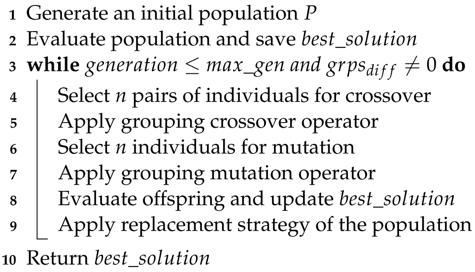
In Algorithm 1, we show the general steps of the GGA proposed in this work. The precise details are shown in the following subsections. The process begins by generating an initial population
P of
individuals created by the population initialization strategy (Line 1). After that, each of the individuals in the population is evaluated, and the best solution for the population is obtained (Line 2). Then, we iterate through a
number of generations or until we find a value equal to zero in the decomposition evaluation. Within this cycle, the individuals to be crossed will be selected, and the offspring will be created through the grouping crossover operator (Lines 4–5). Similarly, the population is updated by the mutation of some individuals in the population (Lines 6–7). Finally, the population is evaluated again to update the population and the best global solution found so far (Lines 8–9).
| Algorithm 1: Grouping Genetic Algorithm for variable decomposition algorithm. |
![Mca 27 00023 i001]() |
In the following subsections, we detail the components and operators of our GGA.
3.1. Genetic Encoding
One of the most important decisions to make while implementing a genetic algorithm is to decide the representation to use to represent the solutions. It has been observed that improper representation can lead to poor performance of the GA. Our GGA works with group-based representation, which is the main characteristic of the GGAs.
Each individual in the population is represented by the groups of variables.
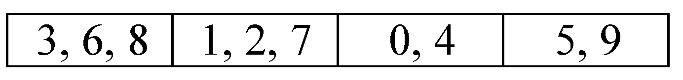
Figure 1 shows an example of an individual that represents a problem with 10 variables numbered from 0 to 9 randomly assigned to four subcomponents or groups. The groups of variables (genes) according to this individual are the following:
,
,
, and
. Note that the number
V of variables in each subcomponent is variable and can be between 1 and
D; in addition, the number of subcomponents
m is between 1 and
D.
3.2. Decomposition Evaluation
Each individual is evaluated to determine its fitness and to discover which one is the best within the population.
Sayed et al. [
3] proposed a decomposition evaluation inspired by the definitions of problem separability [
38] and partial separability [
39]. The definition of problem separability states that a fully separable problem that has
D variables can be written in the form of a linear combination of subproblems of the decision variables, where the evaluation of the complete problem,
, is the same as the aggregation of the evaluation of the subproblems,
, which means
. Additionally, a partially separable problem is defined as one which has
D variables and that can be decomposed into
m subproblems, where the summation of all subproblems equals the solution of the complete problem
such that
,
, where
m is the number of subproblems and
V is the number of variables in the
k-th subproblem. Sayed et al. proposed to measure each decomposition of variables by minimizing the absolute difference between the full evaluation and the sum of each evaluated subgroup.
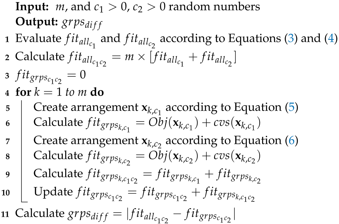
Algorithm 2 shows the decomposition evaluation procedure. First (in Line 1), we obtain
and
through the evaluations of Equations (
3) and (
4), where all the variables take the constant value
and
, respectively. After that, both evaluations are added and multiplied by the number of subgroups in the problem (
m) to obtain
, and then we initialize
as 0 (Lines 2–3). Afterwards, we start a loop from
to the number of subgroups
m in the individual (Lines 4–10), Within this loop, we create two arrangements of
D variables in which each variable belonging to group
k takes the value
, while the remaining variables take the value
to evaluate this arrangement and obtain
. On the other hand, to obtain
, the variables in the
k-th group take the value of
, and the remaining ones take the value of
(Lines 5–8) according to Equations (
5) and (
6). After that, we calculate
as the sum of the previously calculated
and
(Line 9). Thus, to end the loop, we update
as the sum of
and
. Finally, we obtain the evaluation of the decomposition by calculating the absolute difference
shown in Line 11.
| Algorithm 2: Decomposition evaluation. |
![Mca 27 00023 i002]() |
To clarify the decomposition evaluation procedure, we present an example below. Let
be the problem to decompose, and according to the arrangement decomposition given by
,
, and
, we have
. Suppose
and
. In the first step, we calculate
and
. According to Equations (
3) and (
4),
Then, continuing with step 2,
In step 3, we initialize
. Then, we start the for loop. At this point in the process, we have to create arrangement
according to Equation (
5) in step 5 and evaluate it in step 6. Similarly, the process is performed for
in steps 7 and 8. To calculate
the variables of the
k-th group will be evaluated in
, and the rest in
; for
, the group is
, so
and
. A similar calculation is performed with
, but evaluating the variables of the
k-th group in
and the rest in
. Therefore, following the steps into the loop,
For
,
:
For
,
:
For
,
:
The purpose of the problem decomposition is to create the best decomposition; that is, to create independent subcomponents, as well as to minimize the difference
. Therefore, we have adopted a similar evaluation to the one proposed by Aguilar-Justo et al. [
7], which is defined next: to maximize the number of subproblems, the
is updated as follows: (1) if the number of subgroups is one, then the
takes an extreme greater value; (2) if the
is zero, this means that the decomposition is perfect, and it is rewarded by subtracting the number of subgroups (
m) of the individual; (3) in another case, the
value does not change. Since the use of the previous evaluation function benefits a decomposition with a high number of subcomponents, in some cases, a complete decomposition (as many groups as numbers of variables) would be presented as optimal when in reality it is not the case. For this reason, a modification in the evaluation function is necessary (avoiding the benefit to a high number of groups). Therefore, the evaluation function has been modified in our algorithm. This change is summarized in Equation (
7).
3.3. Population Initialization
The initial population in most GGAs is generally generated by obtaining random partitions of the elements to group. In our GGA, to create a new chromosome, a random number between 1 and the dimension of the problem (
D) is generated—i.e.,
—which represents the number of subcomponents
m, and then each variable is randomly assigned to one of these groups. First, we ensure that each group contains at least one variable, and this is done by shuffling the variables and assigning the first
m of them to each group. After that, the remaining variables are randomly assigned to one of the created groups. This is done because in the genetic algorithm DVIIC [
7], a random number is chosen to determine the number of groups, and each variable is randomly assigned to a group (under the integer-based representation).
3.4. Grouping Crossover Operator
After choosing the individuals that are subject to the crossover operator, each pair of these individuals, called parents, will create two new individuals (offspring) through a mating strategy. There are several crossover operators for GGAs; however, for comparison purposes, we have chosen the two-point crossover operator that is analogous to the one used in the genetic algorithm DVIIC [
7]. This operator works as follows: two crossing points (
a and
b) between 1 and the number of genes in the individual minus one (
) are selected randomly to define the crossing section of both parents (
and
). In this way, the first child (
) is generated with a copy of
, injecting and replacing the groups between the crossing points (
a and
b) of
. Next, the groups copied from
with duplicated items are identified, removing the groups and releasing the remaining variables (missing variables), among which are also those elements that were lost when eliminating the groups from the crossing section and were not in the inserted groups. It is important to note that the injected groups remain intact. Finally, the missing variables are re-inserted into a random number of new groups (between 1 and the number of missing variables) to form the complete individual. The second child (
) is generated with the same process but changing the role of the parents.
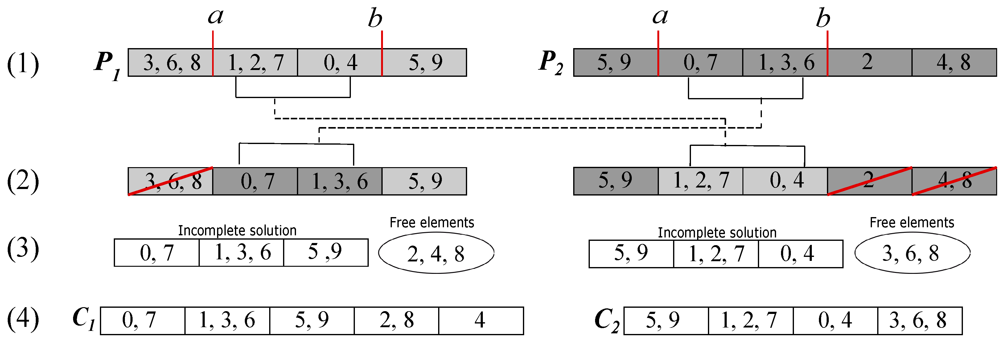
In
Figure 2, we can see an example of crossover for two individuals with 10 variables. The crossing points
a and
b are marked in step (1); then, in step (2), the section between
a and
b of parent
is inserted and replaced in the other parent (
) and vice versa. In step (3), we have the free variables that result from the groups eliminated for having repeated variables, such as, in the first child, the free element 8 that was in the group with 3 and 6, which were repeated elements, and the elements 2 and 4 that were lost variables (elements). Finally, in step (4), we have the offspring with the free elements re-inserted.
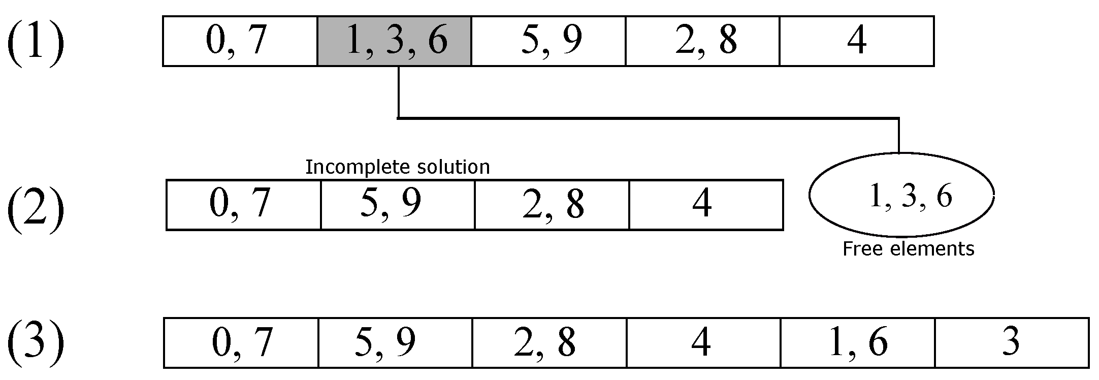
3.5. Grouping Mutation Operator
The mutation operator used in the genetic algorithm DVIIC [
7] is called uniform mutation, in which once an individual is selected to mutate, one of its genes is randomly selected and is changed from the group to which it belongs. Therefore, to take a similar operator, we have chosen to implement the group-oriented elimination mutation operator for GGAs. This operator works by eliminating a random group of the individual. Later, the deleted elements are re-inserted by adding a random number of groups between 1 and the number of free variables, with the variables randomly assigned to them (similar to how an individual is created).
Figure 3 shows an example of the elimination operator. In step (1), the group marked in gray is the eliminated one; then, their elements pass to the free group of elements shown in step (2). Finally, the elements are re-inserted in step (3) with the aforementioned strategy.
3.6. Selection and Replacement Strategies
In a Genetic Algorithm, we have to select the members of the population that will be candidates for crossover and mutation. A selection scheme decides which individuals are allowed to pass on their genes to the next generation, either through cloning, crossover, or mutation. Generally, selection schemes from the literature can be classified into three classes: proportional selection, tournament selection, and ranking selection. Usually, the selection is according to the relative fitness using the best or random individuals [
40,
41].
Several strategies have been proposed for the parent selection (individuals for crossover). In our GGA, we use a selection scheme similar to that included in the genetic algorithm DVIIC [
7], and we carry out a shuffling of the population; for each pair of parents, a random number between 0 and 1 is created. This number determines if the pair of individuals is subject to crossover. That is, the crossover of both individuals is applied when the number is less than or equal to
.
In the same way, the selection of individuals to mutate has been studied, and there are various selection techniques for mutation. In this case, the selection method for mutation is similar to the selection method of the genetic algorithm DVIIC [
7]. Given a mutation probability
, for each individual in the population, a random number between 0 and 1 is generated, and when this number is less or equal than
, the individual will be mutated.
In addition to the selection scheme, there must also be a criterion under which the population will be replaced in each generation. Generally, the replacement strategies can be split into three classes: age-based, fitness-based, and random-based (deleting the oldest, worst, or random individuals, respectively) [
42]. Similar to the strategy of the genetic algorithm DVIIC [
7], in our GGA, after crossover, the offspring replace the parents, and after the mutation, the mutated individuals replace the original ones. Elitism is adopted to always maintain the best solution of the population, replacing the worst individual of the new population.
4. Experiments and Results
In order to study the benefits of using a group-based against an integer encoding in a genetic algorithm, we compared our proposal with the decomposition strategy proposed by Aguilar-Justo et al. [
31]. Therefore, we chose the same set of test functions the authors used. It is the first set for Large-Scale Constrained Optimization Problems and it was proposed by Sayed et al. in 2015 [
3]. This test set has different separability complexity degrees, which are described in
Table 1. It can be tested over three numbers of variables (100, 500, and 1000). These 18 functions were created by combining 6 objective functions with 1, 2, or 3 constraints. The 6 objective functions are based on 2 problems in the literature that have been used, for example, in the CEC 2008 benchmark problems [
4], which are the Rosenbrock’s function, which is multimodal and nonseparable, and the Sphere function, which is unimodal and separable. In addition, in
Table 2, we can see the components of these 18 test functions; that is, the objective function and the constraints that make up each function. The details of the mathematical expression of each function can be consulted in the work of Sayed et al. [
3].
We have compared the results of our GGA against the Dynamical Variable Interaction Identification Technique for Constrained Problems (DVIIC), in which Aguilar et al. [
7] proposed a genetic algorithm for the decomposition of the 18 test functions. We computed 25 independent runs per each benchmark function, in 3 different numbers of variables (100, 500, and 1000). The parameters of our algorithm were set similarly as in the DVIIC work, to compare under equal conditions and perform the same number of function evaluations. These are as follows:
Population size of 100 individuals;
Crossover probability ;
Mutation probability ;
10,000 function evaluations—i.e., 100 generations.
Such a configuration implies that the same number of evaluations is carried out by having 100 individuals in each generation for 100 generations, which is equal to 10,000 evaluations. These experiments were conducted on an Intel(R) Core(TM) i5 CPU with 2.50 GHz, Python 3.4, and Microsoft Windows 10.
In the following tables, we show the results of the execution of our proposed GGA and the genetic algorithm DVIIC. Both were executed for each of the 18 functions, 25 times in each dimension. Furthermore, each of the tables shows the results of the Wilcoxon Rank Sum test for each of the functions (column W). A checkmark (✓) means that there are significant differences in favor of the GGA; in addition, an equality symbol (=) represents there are no significant differences between both algorithms.
First,
Table 3 contains the results according to the evaluation of the best individual for the 25 runs in the 18 functions under 100 variables. The best, median, and the standard deviation registered of the evaluation function (
) value are shown. We can observe that the GGA improves the decomposition evaluation function value in all of the cases compared to DVIIC. As we can see, unlike DVIIC, the GGA reaches the value of 0 in the best result in most cases. Furthermore, the median and standard deviation values obtained by the GGA are smaller in all cases. Such values equal to zero indicate that our algorithm found the best value for the evaluation function (
) in the 25 runs for functions 1 to 12. Finally, the Wilcoxon Rank Sum Test reveals that there are significant differences in favor of the GGA in all cases.
Second,
Table 4 shows the results of our algorithm to solve the same 18 functions, now with 500 variables. The GGA obtained the smallest values in most cases for the best, median, and standard deviation when compared against DVIIC. In a similar way as in
Table 3, the standard deviation and median values equal to zero indicate that our algorithm found the best value for the evaluation function (
) in the 25 runs for functions 1 to 12. Moreover, in the other test functions, the best, median, and standard deviation values are smaller when compared to DVIIC. On the other hand, the Wilcoxon Rank Sum test shows that there are no significant differences between the two algorithms in function 1 and shows significant differences in favor of the GGA in the remaining 17 functions. According to this test, in functions 2 to 18, the Wilcoxon Rank Sum test rejects the hypothesis that the DVIIC approach is as effective as the proposed GGA approach, and
is trivial to solve by the two algorithms.
Finally,
Table 5 contains the results for the 18 functions with both algorithms implemented on 1000 variables. In this experiment, we observed that, in a similar way to the experiment with 500 variables, our GGA obtained the smallest best, median, and standard deviation values in most cases. On the other hand, the behavior of the median and standard deviation values allows us to see that we obtained the zero value in the 25 independent runs for the first 12 functions. Moreover, the Wilcoxon Rank Sum test results show that there are no significant differences between the two algorithms in function 1 and indicate significant differences in favor of the GGA in the remaining 17 functions. In a similar way as in the results with 500 variables, the Wilcoxon Rank Sum test determines that
is a trivial case and rejects the hypothesis that the DVIIC approach is as effective as the proposed GGA approach for the other 17 remaining functions.
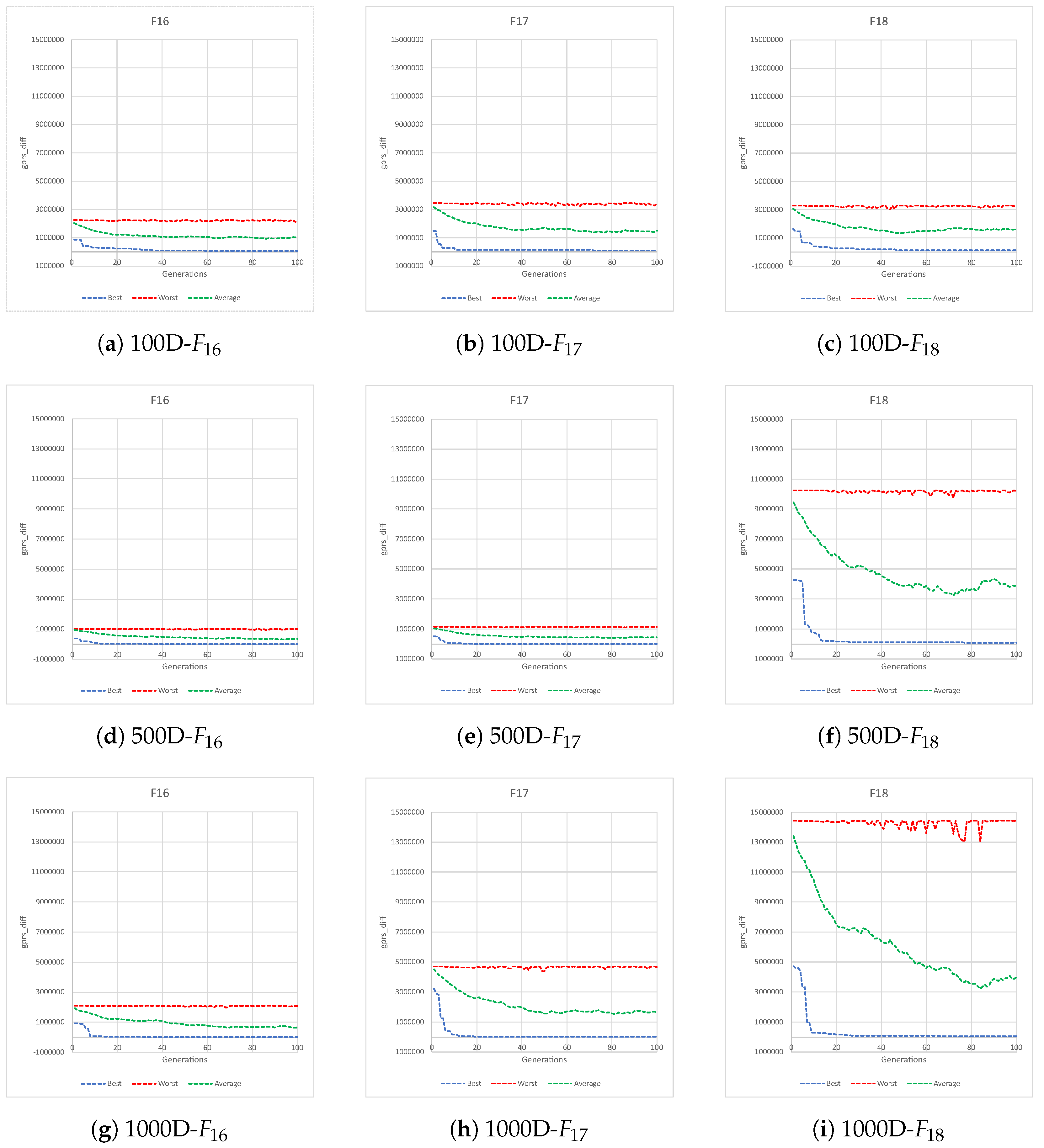
Given the previous tables, we observe that our algorithm presents better performance than DVIIC, obtaining better values in all cases (in comparison with the mentioned algorithm). An interesting behavior is observed in these experiments; it seems to be more difficult for our algorithm to find the minimum decomposition evaluation in the 18 test functions as the dimension decreases. Zero best, median, and standard deviation values of the 25 independent runs indicate a stable behavior of our algorithm in each execution of the first 12 functions of the benchmark (in the three experiments). However, these values increase with the complexity of the functions, and in the end, functions 16, 17, and 18 do not reach the minimum in any of the experiments.
5. Conclusions and Future Work
In this paper, we have proposed a Grouping Genetic Algorithm (GGA) to deal with the decomposition of variables in Large-Scale Constrained Optimization Problems to create subproblems of the original problem and thus reduce the dimension. To evaluate the impact of the representation scheme on the performance of a genetic algorithm, our GGA was designed in a similar way to a state-of-the-art genetic algorithm that works with the decomposition of variables and which includes an integer-based representation. The main difference between the two algorithms was the genetic encoding. The experiments were carried out in a benchmark of 18 functions with different complexity characteristics, and these functions were tested in 100, 500, and 1000 dimensions.
The obtained results confirm that the use of a group-based genetic encoding allows our GGA to obtain good and robust decompositions on test functions with different features and separability complexity degrees, outperforming in all the benchmark functions the results obtained by a genetic algorithm with an integer-based encoding.
We are aware that there are still test functions with spliced nonseparable and overlapping variables that show a high degree of difficulty; for these functions, the included strategies in the GGA do not appear to lead to better solutions. However, the GGA presented in this work does not include the state-of-the-art grouping genetic operators.
Future work will consist of studying the parameters of the GGA as well as the effect of each of the methods used in the crossover and mutation operators to identify the best strategies that work together with the grouping encoding scheme and the features of the functions. Furthermore, it is necessary to implement an efficient reproduction technique with a balance in selective pressure and population diversity to avoid the premature convergence of the best individuals and increase the algorithm’s performance.
The introduction of a new decomposition method opens up an interesting range of possibilities for future research. Currently, we are working on including our GGA in the decomposition step of two Cooperative Co-Evolution methods that include different strategies for the optimization and cooperation of the subcomponents, with the respective feasibility and computational complexity analysis.
Finally, although the set of test functions analyzed in this work is varied concerning the characteristics of the functions, we would explore the proposal in other Large-Scale Constrained Optimization benchmarks.


