Article

Fixed- and Variable-Temperature Kinetic Models to Predict Evaporation of Petroleum Distillates for Fire Debris Applications

by
John W. McIlroy
1,†,
Ruth Waddell Smith
2,* and
Victoria L. McGuffin
1,*
1
Department of Chemistry, Michigan State University, East Lansing, MI 48824, USA
2
Forensic Science Program, School of Criminal Justice, Michigan State University, East Lansing, MI 48824, USA
*
Authors to whom correspondence should be addressed.
Current address: Drug Enforcement Administration, 10150 Technology Blvd., Dallas, TX 75220, USA.
Separations 2018, 5(4), 47; https://doi.org/10.3390/separations5040047
Submission received: 15 July 2018 / Revised: 1 September 2018 / Accepted: 3 September 2018 / Published: 25 September 2018
(This article belongs to the Special Issue Advances in Fire Debris Analysis)

Abstract

:
Forensic fire debris analysis focuses on the identification of a foreign ignitable liquid in debris collected from the scene of a suspected intentional fire. Chromatograms of the extracted debris are compared to a suitable reference collection containing chromatograms of unevaporated and evaporated ignitable liquids. However, there is no standardized method for the evaporation of ignitable liquids and the process itself can be time consuming, which limits the number of chromatograms of evaporated liquids included in the reference collection. This work describes the development and application of a variable-temperature kinetic model to predict evaporation rate constants and mathematically predict chromatograms corresponding to evaporated ignitable liquids. First-order evaporation rate constants were calculated for 78 selected compounds in diesel, which were used to develop predictive models of evaporation rates. Fixed-temperature models were developed to predict the rate constants at five temperatures (5, 10, 20, 30, 35 °C), yielding a mean absolute percent error (MAPE) of 10.0%. The variable-temperature model was then created from these data by multiple linear regression, yielding a MAPE of 16.4%. The model was applied to generate a reference collection of predicted chromatograms of diesel and kerosene corresponding to a range of evaporation levels. Using the modeled reference collection, successful identification of the liquid and level of evaporation in a test set of chromatograms was demonstrated.

1. Introduction

The determination of an intentional rather than accidental fire typically relies on the identification of a foreign ignitable liquid in debris collected from the scene. To identify liquids present in fire debris samples, extracts of the collected debris are analyzed by gas chromatography-mass spectrometry (GC-MS). The resulting total ion chromatogram (TIC) and extracted ion profiles (EIPs) of characteristic compound classes are then compared to reference collections of ignitable liquid chromatograms to identify any liquid present [1]. Despite guidelines for the extraction and analysis of fire debris samples and the interpretation of the resulting chromatograms [1,2,3,4,5,6], identification of liquids is often challenging due to the inherent complexity of the samples. Any liquid present is subjected to the elevated temperatures reached during the fire, resulting in evaporation, while substrates present (e.g., carpeting, clothing, other household materials, etc.) may undergo thermal degradation and/or pyrolysis, which further complicates the resulting chromatogram [7]. While all of these chemical processes contribute to the complexity of the resulting TICs, the focus in this work is specifically on evaporation.
Given that the volatility of liquids is commonly used as accelerants in setting intentional fires, evaporation causes substantial chemical changes such that the chromatogram of the evaporated sample no longer resembles that of the unevaporated liquid. To mitigate this issue, there is general agreement that reference collections should include TICs of liquids evaporated to a few different levels by mass or by volume [1,7]. However, the methods by which liquids are evaporated vary considerably [7,8,9,10,11]. For example, evaporations may be conducted at room temperature or at slightly elevated temperatures and may be conducted passively or actively, with a gentle stream of nitrogen and agitation of the liquid [7,8,9,10,11]. Further, experimental evaporations can be time consuming (e.g., 130 days to passively evaporate gasoline to 93–95% of the original volume [8]), such that including TICs of every liquid evaporated to numerous levels in a reference collection is impractical.
Because of the difficulties in experimental evaporation, the focus in this work was to kinetically model the evaporation process and mathematically predict chromatograms corresponding to different evaporation levels. Models have previously been developed to predict evaporation, although primarily for environmental applications rather than forensic fire debris applications. These models range from simple empirical models [12,13] to complex models that require the estimation of physical properties from distillation data [14,15,16].
Evaporation rates have also been predicted using first-order kinetic models [17,18,19,20]. Smith developed a model to predict the evaporation rate constant using vapor pressure and the mass transfer coefficient [19]. However, the experiments in this work were only conducted on simple mixtures of two compounds and at a single temperature. In the work by Regnier and Scott, the evaporation rate constants of normal alkanes were correlated with vapor pressure [18]. The vapor pressure of each compound was related to temperature through the Clausius-Clapeyron equation. While the success of both kinetic models in predicting evaporation rate constants was demonstrated, the identities, concentrations, and physical properties of the compounds in the liquid must be known [18,19]. Identification of all constituents in complex ignitable liquids, particularly isomeric compounds, remains challenging and the physical properties for many of the relevant compounds are not available in the literature.
A kinetic-based model that overcomes these limitations was previously developed in our laboratory [17]. Evaporation rate constants for representative compounds in diesel were determined empirically at 20 °C and plotted as a function of retention index. Linear regression was applied to define the model, which was then used to predict evaporation rate constants as a function of retention index. Retention index is a useful surrogate for physical properties such as vapor pressure or boiling point, as it can be readily determined without requiring knowledge of the identity or concentration of compounds in the liquid. The success of the kinetic-based model in predicting chromatograms corresponding to evaporated petroleum distillates has also been demonstrated [21].
As the kinetic model was developed based on empirical evaporation rate constants determined at a fixed temperature, the effect of temperature on the kinetics of evaporation was not taken into account [17,21]. Recent work by Birks et al. reported the unexpected effect of elevated temperature on the evaporation of gasoline, highlighting the importance of temperature in any predictive model [22]. Thus, the work reported herein expands upon our previous efforts by incorporating a variable temperature term into the kinetic model. First, fixed-temperature models were developed at five temperatures and the error in predicting evaporation rate constants was determined. These data were then used to develop the variable-temperature model and prediction errors were calculated for comparison to the fixed-temperature models. Finally, the variable-temperature model was used to predict evaporation rate constants and generate chromatograms corresponding to evaporated petroleum distillates to demonstrate practical application for fire debris analysis.

2. Theory

The model developed in our initial work is based on first-order kinetics, the equation for which is shown below,
C t = C 0   exp ( k   t )
where the concentration (Ct) of a compound at time (t) is related to the initial concentration (C0) and the rate constant (k) for evaporation. In our previous work, diesel was evaporated under controlled temperature and humidity conditions as a function of time and the evaporated samples were analyzed by GC-MS [17]. The normalized abundances of more than 70 compounds representing different compound classes (e.g., normal alkane, branched and cyclic alkane, alkyl aromatic, and polycyclic aromatic) within the diesel were plotted versus time. The resulting decay curves for each compound were fit to Equation (1) to determine the evaporation rate constants.
For each compound identified in the evaporated diesel samples, the retention index (IT) was calculated which, for a given compound under temperature-controlled conditions, is given by Equation (2),
I T = 100 [ t R , i T t R , z T t R , z + 1 T t R , z T + z ]
where the retention time of the compound (tTR,i) is expressed relative to the retention time of the normal alkanes of carbon number z that elute before (tTR,z) and after (tTR,z+1) the compound [23,24,25]. As IT is independent of most gas chromatography conditions, including column dimensions, temperature, flow rate, etc., this parameter is more consistent between different instruments and different laboratories.
The empirically derived rate constants of compounds in the evaporated diesel samples were plotted as a function of IT and linear regression was applied to define the kinetic model (Equation (3)),
ln ( k ) = m   I T + b
where m and b are the slope and intercept, respectively, of the regression plot [17]. Class-specific models were developed for the normal alkane, branched and cyclic alkane, alkyl aromatic, and polycyclic aromatic compound classes within diesel. Errors in predicting evaporation rate constants using each class-specific model ranged from 4.0–8.2%. A comprehensive model incorporating all compound classes was developed, with only a slightly higher prediction error of 10%.
The model has clear potential for fire debris applications, primarily in its ability to predict chromatograms corresponding to different evaporation levels of a given liquid. However, to this point, the model has only been used to predict evaporation rate constants and modeled chromatograms at a fixed temperature of 20 °C. For practical applications, it is critical to include temperature as a variable because evaporation rates are strongly dependent on temperature. Birks et al. recently reported the unexpected effect of elevated temperatures on the evaporation of an artificial gasoline mixture [22]. In their work, a closed-system thermodynamic approach using Antoine coefficients to predict vapor pressure was used to simulate evaporation at temperatures up to 500 °C. As temperature increased, there was a greater relative increase in the vapor pressures of the less volatile components in the mixture compared to the more volatile components. As a result, the gasoline mixture retained a greater fraction of more volatile compounds when evaporated to 95% at 500 °C, compared to the same level of evaporation at 25 °C. While these results indicate the necessity to incorporate temperature into modeling, the current thermodynamic approach requires knowledge of the identity, vapor pressure, and concentration of compounds within the fuel, which may not be possible depending on the chemical complexity of the fuel [22].
In the present work, the kinetic-based model was modified to include a temperature term. According to the Arrhenius equation [26], the natural logarithm of the rate constant is inversely related to absolute temperature (T) according to Equation (4),
ln ( k ) = ln A E a R T
where Ea is the activation energy, R is the gas constant, and A is the pre-exponential factor. By combining Equations (3) and (4), a variable-temperature model to predict the rate constant can be defined according to Equation (5),
ln ( k ) = m 1   I T + m 2 ( 1 T ) + b
where the slopes (m1 and m2) and intercept (b) are determined by multiple linear regression. In the present work, five fixed-temperature models were initially defined and validated. The same data were then used to define and validate the variable-temperature model and to demonstrate applications for fire debris analysis in the form of a modeled reference collection.

3. Materials and Methods

Diesel fuel was used for model development due to its chemical complexity, containing a wide range of compounds (e.g., normal alkanes, branched and cyclic alkanes, alkyl aromatics, and polycyclic aromatics) of varying volatilities. A large volume (~5 gallons) of diesel fuel was collected from a local service station, transferred into acid-washed amber glass bottles, and stored at ~5 °C until analysis. This fuel sample was used over the entire course of the study. Kerosene was used for model validation. Similar to diesel, kerosene was purchased locally and was stored in an amber bottle at ~5 °C until use.

3.1. Evaporation of Petroleum Distillates

Diesel samples were evaporated in an evaporation chamber designed in house [17]. Temperature was controlled by an Ambi-Hi-Lo incubator (5–50 °C ± 0.5 °C, model 3550DT, Lab-Line, Melrose Park, IL, USA) and relative humidity (RH) was controlled by placing trays of water, totaling approximately 300 mL, inside the chamber. Temperature and humidity were monitored and recorded at 2-minute intervals throughout the evaporation process using a data logger (0–55 °C ± 0.3 °C, 10–95% RH ± 5% RH, TR-74Ui, T & D Corporation, Nagano, Japan). Aliquots of diesel (1.0 mL) were delivered into small glass petri dishes (60 mm diameter × 15 mm high) containing distilled water (15 mL), resulting in a thin layer of diesel (~0.5 mm) for evaporation. Petri dishes were transferred to the evaporation chamber and samples were evaporated in triplicate up to 300 h at five different temperatures (5, 10, 20, 30, and 35 °C).
For model validation, additional diesel and kerosene samples were prepared as previously described. For each fuel, an additional three samples were prepared without the water layer: These samples were weighed before and after evaporation at 20 °C for 100 h to determine the evaporative loss by mass.

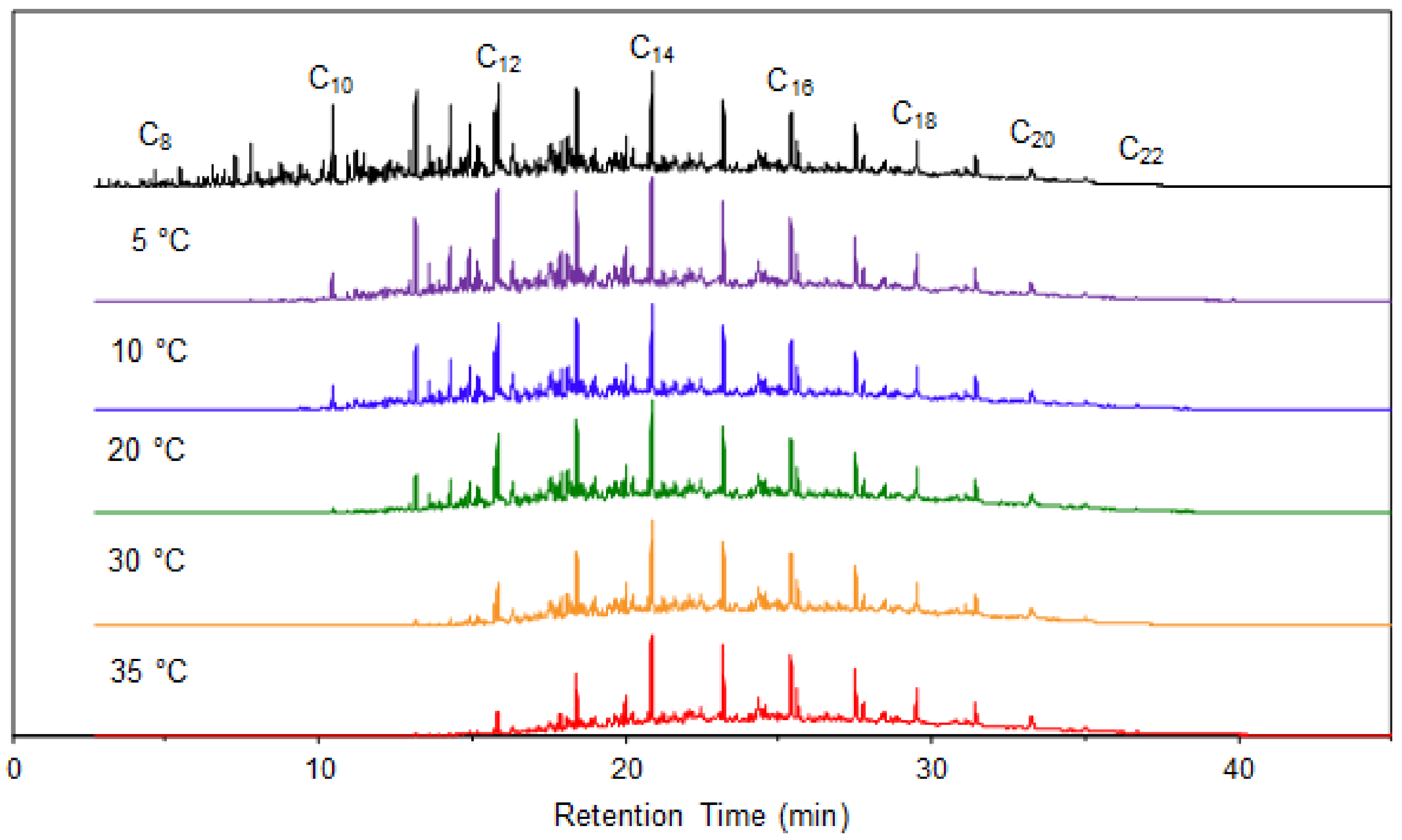
3.2. Gas Chromatography-Mass Spectrometry Analysis

To prepare samples for GC-MS analysis, the contents of the petri dishes (diesel and kerosene) were quantitatively transferred to a separatory funnel and the dish was rinsed several times with approximately 1 mL of dichloromethane. The organic layer was then transferred and diluted in a 10.0 mL volumetric flask. An additional dilution (1:50 v/v) in dichloromethane was performed prior to analysis.
The GC-MS system consisted of an Agilent 7890N gas chromatograph with an Agilent 7693 automatic liquid sampler, coupled to an Agilent 5975 mass spectrometer (all Agilent Technologies, Santa Clara, CA, USA). The GC separation was performed on a capillary column containing a 100% polydimethylsiloxane stationary phase (HP-1MS, 30 m × 0.25 mm × 0.25 μm, Agilent Technologies), using ultra-high purity helium as the carrier gas at a nominal flow rate of 1 mL/min. A 1 µL aliquot of each diluted extract was introduced via a pulsed (15 psi for 0.25 min), split (50:1) injection at 280 °C. The GC temperature program was as follows: Initial temperature 50 °C, ramped up at 5 °C/min to a final temperature of 280 °C, with a final hold for 4 min. The transfer line was held at 300 °C and separated analytes were ionized via electron ionization at 70 eV. Ions were separated using a quadrupole mass analyzer, which scanned mass-to-charge (m/z) ratios of 40–550 at 2.91 scans/s.
Compounds in the diesel samples were identified based on the m/z ratio of prominent ions in the total ion chromatogram (TIC) as well as the GC retention indices [17]. Compounds were quantified based on the abundance from extracted ion chromatograms (EIC), normalized to the abundance of n-heneicosane (C21) in the EIC at m/z 57 for diesel and to the abundance of n-pentadecane (C15) in the EIC at m/z 57 for kerosene.

3.3. Model Development and Validation

The first-order rate constants (k) were determined using the methodology described in our previous work [17]. Briefly, the normalized abundance of each selected compound was plotted as a function of evaporation time, and nonlinear regression was used to fit the resulting decay curves to Equation (1) to determine the evaporation rate constant (TableCurve 2D, version 5.01, Systat Software, Richmond, CA, USA). The characteristic lifetime (τ), which is equal to 1/k, is often used to describe the completeness of the decay curve. Only rate constants for compounds with greater than 0.5 τ in the decay curve were included in model development. With this criterion, a total of 78 compounds were included in model development and a further 29 compounds were included in method validation, while introducing only minimal error of 2.9% [17]. A list of the compounds selected for model development and validation is provided in the Supplementary Material (Table S1a and S1b, respectively).
For each fixed temperature (5, 10, 20, 30, and 35 °C), the natural logarithm of the empirically determined rate constant for each compound was plotted as a function of IT. Linear regression was then performed in Microsoft Excel (Office 2013, version 15.0, Microsoft Corporation, Redmond, WA, USA) to define each model in the form shown in Equation (3). The performance of each fixed-temperature model was evaluated by comparing the rate constants predicted by the models (kpred) to the corresponding experimental evaporation rate constants (kexp) for each selected compound. For each fixed-temperature model, the absolute percent error (APE) in rate constant prediction for each compound was calculated and then averaged across all compounds to yield the mean absolute percent error (MAPE) [27], according to Equation (6),
MAPE = i = 1 n | k exp , i k pred , i k exp , i | n   100
To define the variable-temperature model, the experimentally-derived rate constants for each compound at each temperature were plotted as a function of IT and multiple linear regression was performed in Microsoft Excel (Office 2013, version 15.0, Microsoft Corporation), defining the model in the form shown in Equation (5). The performance of the variable-temperature model was assessed in a similar manner as described for the fixed-temperature models.

4. Results and Discussion

Representative TICs of diesel fuel prior to evaporation and after 300 h of evaporation at 5, 10, 20, 30, and 35 °C are shown in Figure 1. Volatile compounds, such as n-octane (C8), were completely evaporated after 300 h at all temperatures. Less volatile compounds, such as n-tetradecane (C14), remained relatively unchanged at all temperatures, even after 300 h. For compounds eluting between C8 and C14, an increase in temperature resulted in more rapid evaporation, as expected from the Arrhenius equation (Equation (4)). For example, at 10 °C, n-decane (C10) was still observed in the TIC, albeit at low abundance; however, at temperatures above 20 °C, C10 was completely evaporated. The empirically determined evaporation rate constants at each temperature for all selected compounds are summarized in the Supplementary Material (Tables S2a–S6a). These experimental data were then used to develop fixed-temperature and variable-temperature models, as described in the following sections.

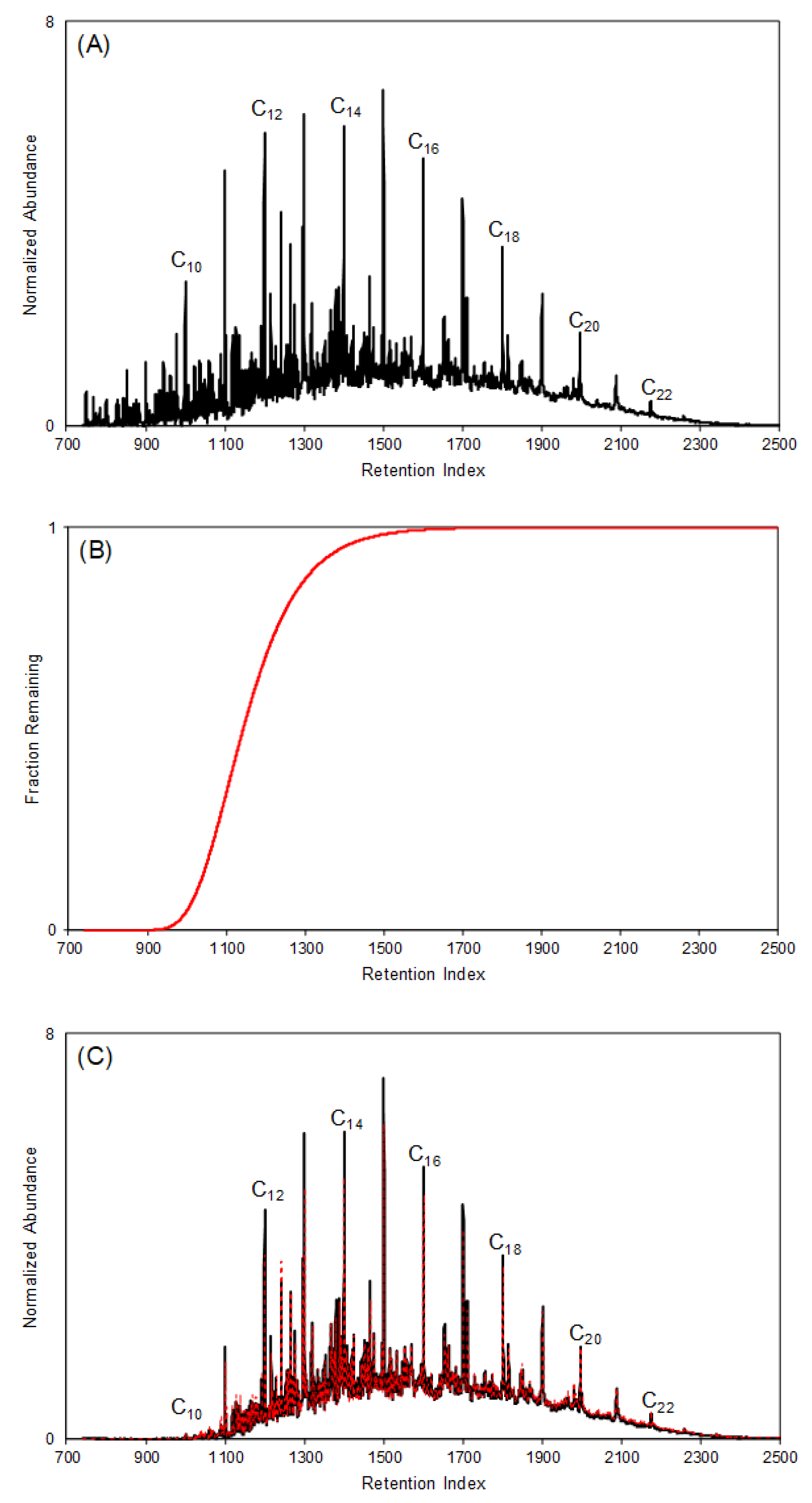
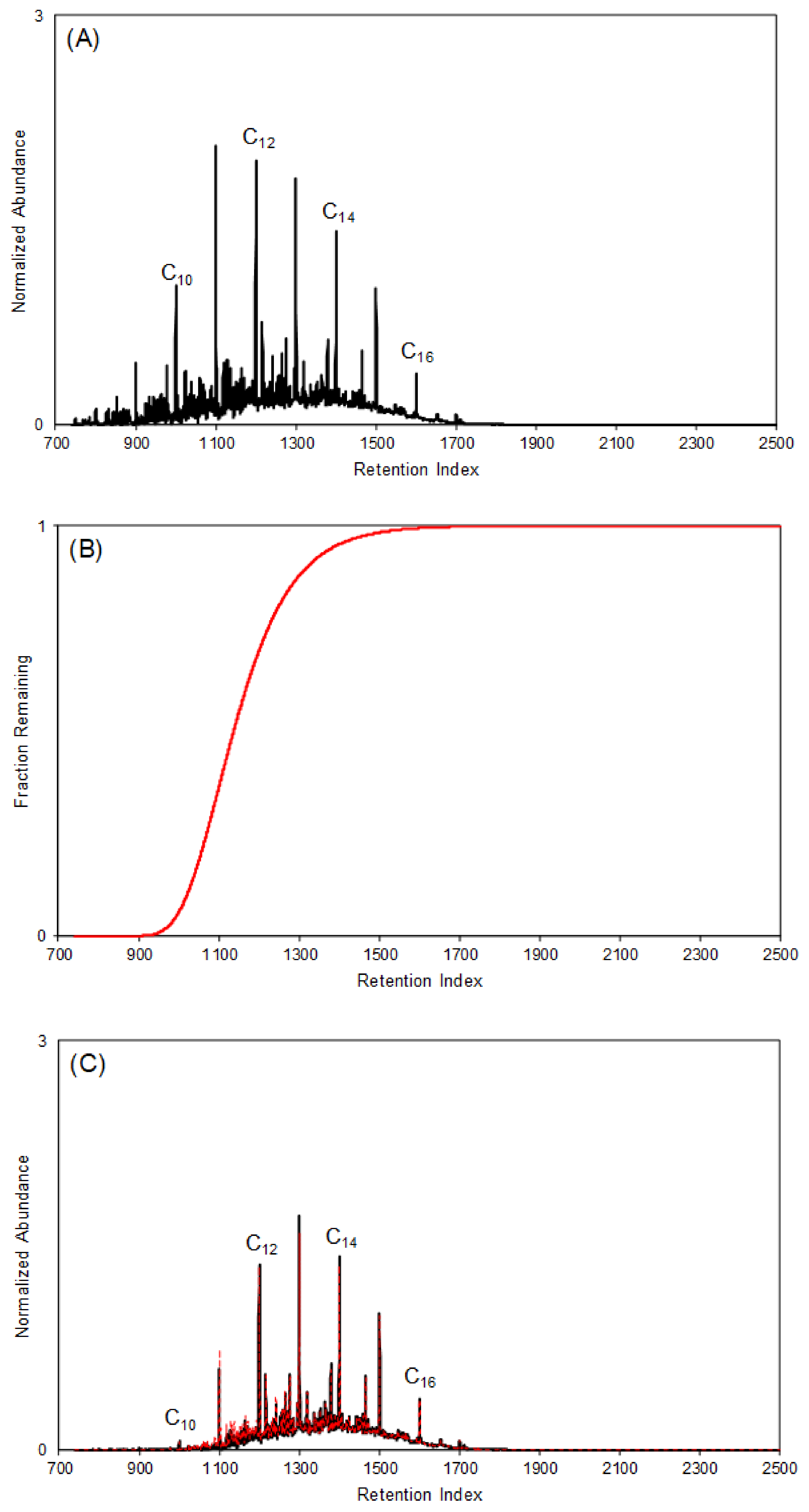
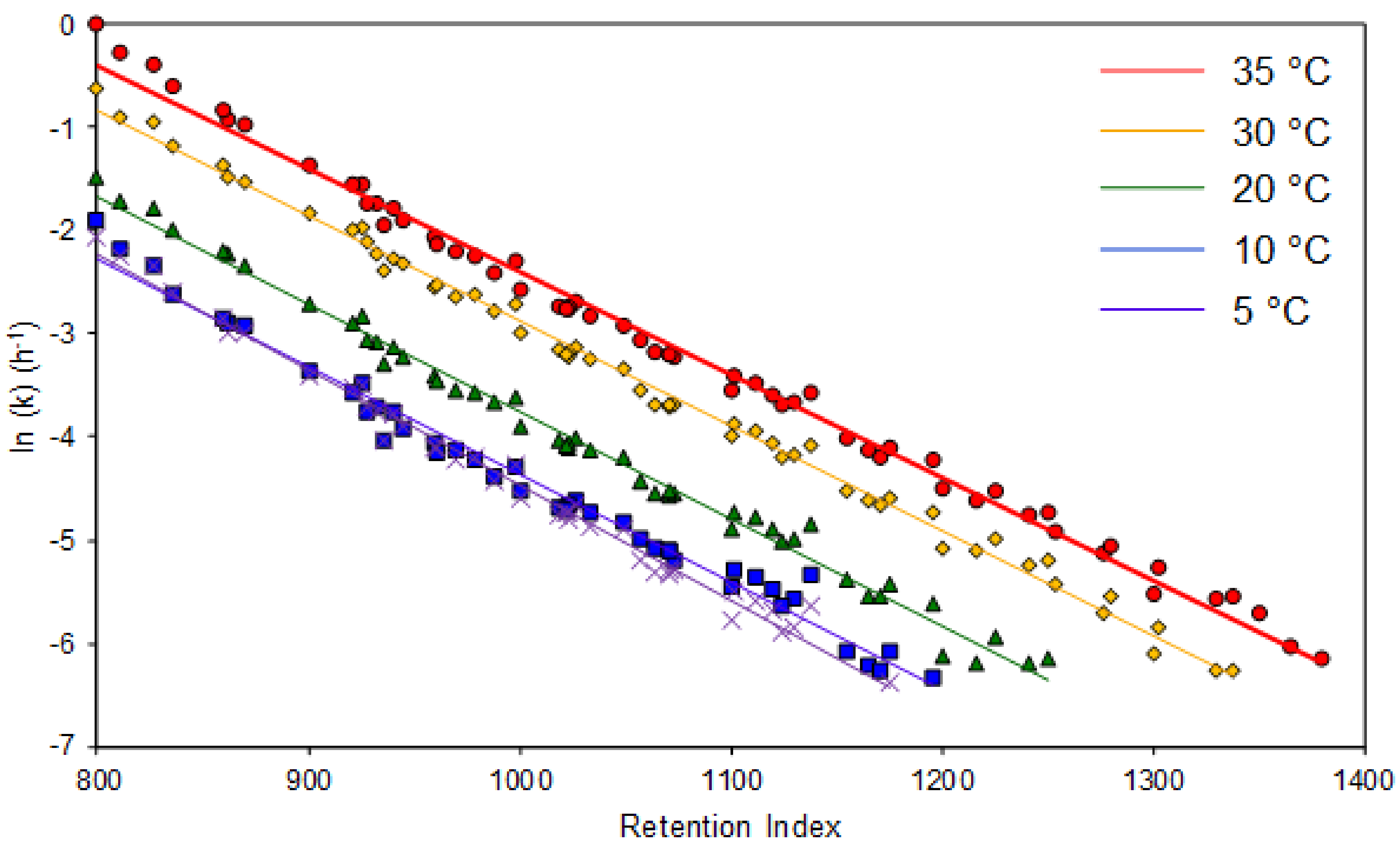
4.1. Fixed-Temperature Models

The natural logarithm of the rate constant (ln (k)) for each compound at each temperature was plotted versus IT, as shown in Figure 2. Linear regression was used to calculate the slope (m) and intercept (b) of Equation (3) to determine the fitting coefficients for each model, as summarized in Table 1. At all temperatures, a high coefficient of determination (R2 = 0.982–0.995) indicated a good quality of fit to the linear equation. It is noteworthy that the slopes and the intercepts of Equation (3) show some degree of temperature dependence: As temperature increases, both the slope and intercept increase from −1.12 × 10⁻² and 6.78 at 5 °C to −1.00 × 10⁻² and 7.62 at 35 °C. The APE in predicting the rate constant for the selected compounds ranged from 0.0–40.6% across all fixed-temperature models (Supplementary Material, Tables S2a–S6a). The MAPE (Equation (6)) for each fixed-temperature model ranged from 8.6–10.8%, with an overall average prediction error of 10.0% (Table 1).
To validate the fixed-temperature models, 29 additional compounds were selected that spanned a similar IT range as those used to develop the models. The rate constants were experimentally determined at the same temperatures (5, 10, 20, 30, and 35 °C) and are summarized in the Supplementary Material (Tables S2b–S6b). The experimental rate constants were then compared to the values predicted by the fixed-temperature models at the corresponding temperature. As a representative example, the experimental and predicted rate constants for decalin (IT = 1045) at each temperature are shown in Table 2. For this compound, the APE for each fixed-temperature model ranged from 0.5–17%, with an overall average of 8.8%.
The APE in predicting the rate constant for all validation compounds ranged from 0.0–52.4% across all fixed-temperature models (Supplementary Material, Tables S2b–S6b). Taking all 29 validation compounds into account, the MAPE (Equation (6)) for each fixed-temperature model ranged from 7.6–13.4%, with an overall average of 10.1% (Table 3), which is comparable to the MAPE of 10.0% that was determined during model development (Table 1). The difference in prediction error of only 0.1% demonstrates the applicability of the fixed-temperature models to a wider range of compounds, not only those used to develop the models. The ability to apply the model to additional compounds is essential for future applications beyond diesel and, in the future, beyond petroleum distillates.

4.2. Variable-Temperature Model

The models developed in Section 4.1 were generated for five fixed temperatures (5–35 °C), but do not include temperature as a variable. Using the same experimental data, a variable-temperature model was developed to predict the rate constant using Equation (5). Multiple linear regression was performed to determine the fitting coefficients for the slopes (m1 and m2) and the intercept (b), defining the variable-temperature model as shown in Equation (7),
ln ( k ) = 0.0103   I T 6410   ( 1 T ) + 28.7
From Equation (7), the slope m1 is comparable to that for the fixed-temperature models (Table 1), indicating a similar dependence of rate constant on retention index. However, slope m2 has a larger value, indicating a strong dependence of rate constant on temperature. The coefficient of determination for the variable-temperature model (R2 = 0.979) was only slightly lower than the coefficients determined for the fixed-temperature models (R2 = 0.982–0.995, Table 1). The performance of the variable-temperature model was evaluated by comparing the rate constant predicted using the model (Equation (7)) to the rate constants determined experimentally at each temperature. The APE for each selected compound is summarized in the Supplementary Material (Tables S2a–S6a) and ranged from 0.2–70.5%. The MAPE is summarized in Table 1, and ranged from 9.4–26%, with an overall average of 16.4%, which was slightly higher than the average error of 10.0% determined using the fixed-temperature models.
The rate constants for the 29 validation compounds were also predicted at each temperature using the variable-temperature model. Again, taking decalin (IT = 1045) as an example, the APE at each temperature ranged from 0.3–30%, with an average error of 13% for the variable-temperature model, which was higher than the average error of 8.8% determined using the fixed-temperature models (Table 2). The APE for all validation compounds is summarized in the Supplementary Material (Tables S2b–S6b) and ranged from 0.2–54.1%, consistent with the prediction errors associated with the fixed-temperature models (0.0–52.4%).
The MAPE for all 29 validation compounds at each temperature is summarized in Table 3 and ranged from 10.8–27.5%, with an overall average of 16.8% for the variable-temperature model (compared to 10.1% for the fixed-temperature models, Table 3). Again, the error observed for the validation compounds is consistent with that for the compounds used to develop the model (Table 1).
It is useful to consider the source and magnitude of these prediction errors. Kinetic measurements are, by nature, less precise and accurate than equilibrium measurements, as the values change as a function of time and cannot be averaged. In this study, the precision of individual measurements by GC-MS ranged from approximately ±1–10%, depending on abundance. For ±1% precision, the resulting precision of the rate constant is expected to vary from 2.1–26% for rate constants ranging from 1 × 10⁻² to 1 × 10⁻³ h−1, respectively, by propagation of error via Equation (1). For ±10% precision, the resulting precision of the rate constant is an order of magnitude larger at 21–260%. Hence, most of the uncertainty in the rate constants arises from imprecision in the GC-MS abundance measurements.
In addition, a single model was used to predict rate constants for all compounds, regardless of chemical class. The prediction accuracy could be improved if separate models were developed for each compound [17]; however, such practice would be impractical for forensic applications. Finally, the prediction errors are slightly higher for the variable-temperature model than for the fixed-temperature model, as the regression equation includes an additional, uncorrelated variable. Nevertheless, the variable-temperature kinetic model is broadly applicable to a wide range of compounds and performance is comparable to that of the fixed-temperature models.

4.3. Applications of Variable-Temperature Model

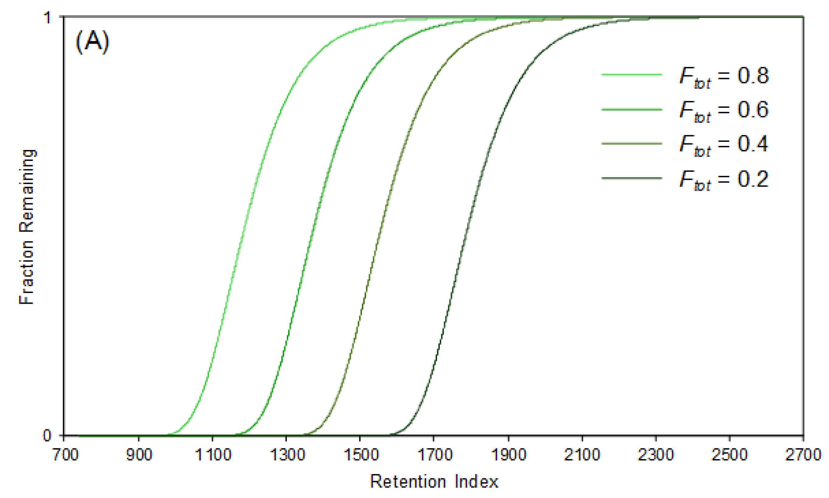
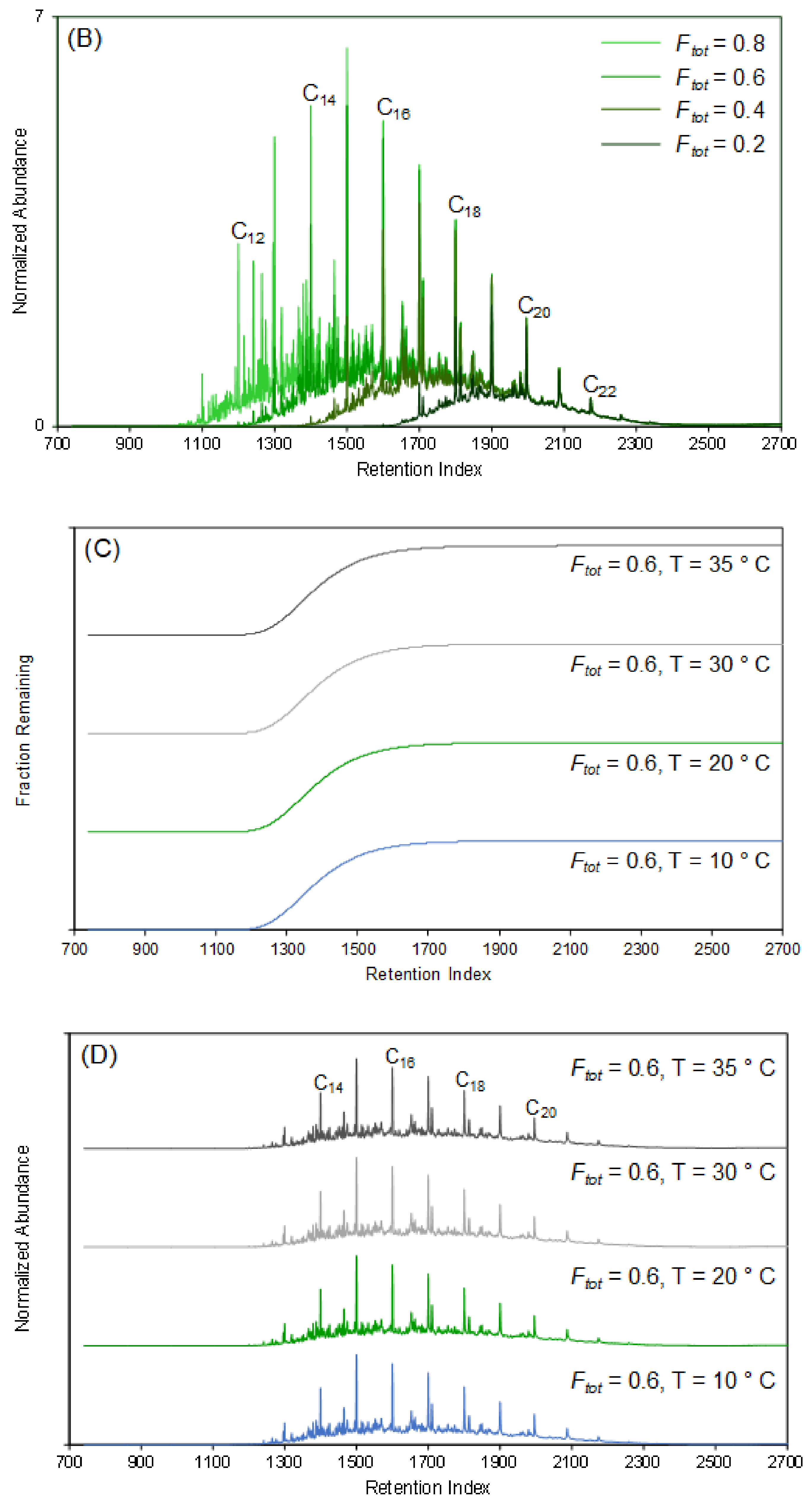
4.3.1. Predicting the Fraction Remaining of Petroleum Distillates at a Given Time and Temperature

The evaporation rate constants predicted by the models can be used to determine the fraction remaining of an individual compound at a given retention index (FIT). As an example, for the variable-temperature model, FIT is obtained by substituting Equation (7) into Equation (1) and rearranging, as shown in Equation (8),
F I T = C I T , t C I T , 0 = exp (   exp ( 0.0103   I T 6410 ( 1 T ) + 28.7 )   t )
the total fraction remaining (Ftot) of the fuel is then determined by summing Equation (8) over the relevant IT range from the initial to final retention index ( I i T to I f T ), as shown in Equation (9),
F tot = j = I i T I f T F j C j , 0 j = I i T I f T C j , 0
as concentration is proportional to abundance in GC-MS, the initial concentration (Cj,0) at each retention index can be determined from the abundance in the TIC or EIP of an unevaporated sample.
The application of the variable-temperature model to predict the chromatogram of a diesel sample evaporated at 20 °C (293 K) for 100 h is shown in Figure 3. First, an unevaporated diesel sample was analyzed and the resulting TIC is shown in Figure 3A. The FIT was predicted using the variable-temperature model (Equation (8)) with T = 293 K and t = 100 h and plotted as a function of IT to generate the fraction-remaining curve (Figure 3B). The FIT ranges from 0–1, with FIT = 0 indicating complete evaporation at that IT, FIT = 1 indicating no evaporation, and FIT values between these two limits indicating different extents of evaporation. From the fraction-remaining curve for diesel (Figure 3B), any compound with IT < 900 is predicted to be completely evaporated (FIT = 0), compounds with IT between 900 and 1650 are expected to undergo evaporation to differing extents, and compounds with IT > 1650 are predicted to be relatively unaffected by evaporation (FIT = 1).
The fraction-remaining curve (Figure 3B) was then multiplied by the TIC of the unevaporated diesel (Figure 3A) to generate the predicted chromatogram of the evaporated diesel (red dotted line in Figure 3C). The predicted chromatogram was compared to the chromatogram of a diesel sample evaporated experimentally at 20 °C for 100 h (black solid line in Figure 3C) using Pearson product-moment correlation (PPMC) coefficients to assess similarity. The PPMC coefficient (r) measures how two variables (x and y) change with respect to one another (covariance), compared to the degree to which each variable changes independently (variance), as shown in Equation (10),
r = [ ( x i x ¯ ) ( y i y ¯ ) ] ( x i x ¯ ) 2   ( y i y ¯ ) 2
the PPMC coefficients range from +1, which indicates a perfect positive correlation, to −1, which indicates a perfect negative correlation. Correlations can be classified as strong (0.8 ≤ |r| ≤ 1), moderate (0.5 < |r| < 0.8), or weak (0 ≤ |r| ≤ 0.5) [28]. In relation to chromatograms, xi and yi represent the abundance at each retention index in chromatograms x and y, respectively, and x ¯ and y ¯ represent the mean abundance of all points in chromatograms x and y, respectively.
The predicted and experimentally derived diesel chromatograms were strongly correlated with a mean PPMC coefficient of 0.998 ± 0.001 (based on n = 27 comparisons of predicted and experimental chromatograms). The high PPMC coefficient indicates that the distribution of compounds in the predicted chromatogram is very similar to the distribution in the experimental chromatogram. However, as PPMC coefficients are insensitive to total abundance, the predicted and experimental chromatograms were also assessed based on Ftot, which indicates the total abundance represented in each chromatogram.
For the evaporated diesel, the experimentally determined Ftot by mass was 0.82. For the predicted chromatogram, the Ftot (Equation (9)) was 0.84, yielding an absolute error in prediction of 3.1%. However, the predicted Ftot calculation was based on the change in peak abundance between the chromatograms of the predicted evaporated and the unevaporated samples, whereas the experimental fraction remaining was based on the difference in mass before and after evaporation. Thus, the experimental Ftot was also calculated based on the area under the chromatograms of the evaporated and unevaporated samples (Ftot by area). In this case, the Ftot by area was 0.88, yielding a slightly higher absolute error of 3.7%.
One of the advantages of this model is that the same regression equations (Equations (7) and (8)) can be applied, in principle, to any petroleum distillate. To demonstrate this capability, the variable-temperature kinetic model was applied to predict chromatograms corresponding to kerosene evaporated at 20 °C for 100 h. Kerosene was also experimentally evaporated under these conditions for comparison to the modeled chromatogram.
A representative chromatogram of the unevaporated kerosene is shown in Figure 4A. Kerosene contains a similar distribution of compounds as diesel, although it does contain more short-chain normal alkanes, which increases the volatility compared to diesel. With the similarity in chemical composition, the fraction remaining curve for kerosene (Figure 4B) is very similar to the curve for diesel (Figure 3B): compounds with IT < 900 are predicted to be completely evaporated, compounds with IT > 1600 are predicted to be relatively unaffected by evaporation, and compounds with IT between these two limits are predicted to undergo evaporation to different extents.
The fraction-remaining curve (Figure 4B) was then multiplied by the TIC of the unevaporated kerosene (Figure 4A) to generate the predicted chromatogram of evaporated kerosene (red dotted line in Figure 4C). The resulting predicted chromatogram showed a high degree of similarity with the chromatogram for the experimentally evaporated liquid (black solid line in Figure 4C). However, the more volatile compounds (IT < 1200) were at slightly higher abundance in the predicted chromatogram, whereas less volatile compounds (IT > 1200) were at slightly higher abundance in the experimental chromatogram. Nonetheless, the mean PPMC coefficient between the predicted and experimentally derived chromatograms was 0.987 ± 0.001 (based on n = 34 comparisons), indicating strong correlation. The experimental Ftot by mass was 0.62, whereas the predicted Ftot was 0.69, yielding an absolute error in prediction of 12.6%. However, the experimental Ftot by area was 0.65, yielding a lower prediction error of 6.5%.
Despite strong correlation between predicted and experimentally derived chromatograms, PPMC coefficients for kerosene (r = 0.987) were lower than those observed for diesel (r = 0.998) and the error in Ftot was greater (Ftot = 6.5% compared to 3.7% for diesel). A possible source of this discrepancy lies in the normalization procedure. For diesel, n-heneicosane (C21), a nonvolatile compound unaffected by evaporation, was selected for normalization. However, C21 was not present in kerosene and, accordingly, the kerosene chromatogram was normalized to n-pentadecane (C15). As C15 is notably more volatile than C21, any significant evaporation of C15 would introduce a systematic error in the predictions.
Even with this noted limitation, the experimental chromatograms for kerosene are strongly correlated with the chromatograms generated using the variable-temperature model, which demonstrates the wider applicability of the model beyond diesel. The low prediction errors further demonstrate the success of the model in generating chromatograms corresponding to evaporated liquids.

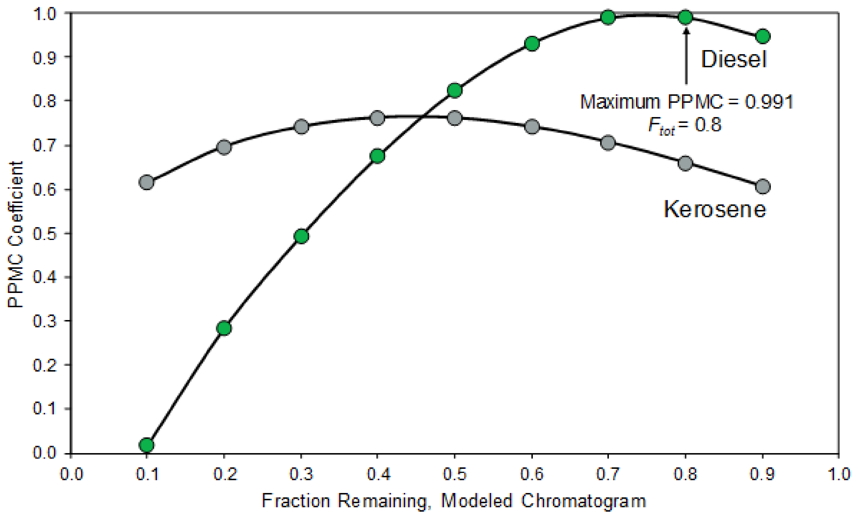
4.3.2. Generating Modeled Reference Collection to Identify Ignitable Liquids in Fire Debris

In Section 4.3.1, the variable-temperature model was used to predict chromatograms corresponding to a given evaporation temperature and time for the purposes of validation. However, a more practical application of the model for fire debris analysis is to predict chromatograms corresponding to different Ftot levels, which can be expressed in terms of the evaporation level of the fuel. For example, a chromatogram corresponding to Ftot = 0.9 represents 90% remaining of the fuel, which is equivalent to 10% evaporated fuel. In turn, the predicted chromatograms could form the basis of an extensive reference collection that could be used as a tool to aid in ignitable liquid identifications.
To demonstrate this application, the variable-temperature model was used to generate predicted chromatograms corresponding to Ftot values ranging from 0.9–0.1, in increments of 0.1, at four temperatures (10, 20, 30, and 35 °C) for both diesel and kerosene. To do this, FIT was calculated using Equation (8) and Ftot was calculated by summation across the IT range (i.e., ITi = 739 and ITf = 3238) using Equation (9) at each temperature. The variable t in Equation (8) was then altered to attain the desired Ftot value. For example, for T = 20 °C, setting t = 40 h resulted in Ftot = 0.9, whereas setting t = 450,000 h resulted in Ftot = 0.1. The fraction-remaining curves (Figure 5A) were individually multiplied by the chromatogram of an unevaporated diesel to generate the predicted chromatograms corresponding to the different Ftot values (Figure 5B). Note that for clarity in Figure 5A,B, fraction-remaining curves and predicted chromatograms are shown only for the even Ftot values at a single temperature (T = 20 °C).
As Ftot decreases, the fraction-remaining curves shift to the right on the retention index axis (Figure 5A). That is, for Ftot = 0.8 at 20 °C, all compounds with IT < 900 are expected to be completely evaporated, whereas for Ftot = 0.2 at 20 °C, all compounds with IT < 1600 are expected to be completely evaporated (Figure 5A). These differences are reflected in the distribution of compounds observed in the predicted chromatograms for the evaporated diesel (Figure 5B): n-alkanes in the range C11–C22 are observed for Ftot = 0.8 but, as Ftot decreases to 0.2, only the less volatile alkanes in the range C17–C22 remain.
Similar trends were observed for the fraction-remaining curves and predicted chromatograms generated at each temperature for each Ftot value. As a representative example, the fraction-remaining curves corresponding to Ftot = 0.6 for diesel at each temperature are shown in Figure 5C and the corresponding predicted chromatograms are shown in Figure 5D. The fraction-remaining curves and hence, the predicted chromatograms, are remarkably similar at each temperature suggesting that evaporation is similar, irrespective of temperature. However, it should be noted that the temperature range considered here is relatively narrow, spanning only 25 °C.
The chromatograms of each liquid predicted using the variable-temperature model in this manner constituted the modeled reference collection (n = 72, chromatograms for two fuels at nine evaporation levels and four temperatures) that was subsequently used in further comparisons. Two test sets of experimentally derived chromatograms were generated for comparison with the modeled reference collection. The first test set (Test Set 1) consisted of 10 chromatograms of diesel experimentally evaporated at 35 °C for times ranging from 1.5–300 h. Test Set 1 also included chromatograms of instrument replicates (n = 3) and evaporation replicates (n = 2). The second test set (Test Set 2) contained 10 chromatograms of diesel experimentally evaporated at the four different temperatures for times ranging from 0.5–150 h. Chromatograms in Test Set 2 were randomly selected using the random number generator function in Microsoft Excel (Office 365, version 1804, Microsoft Corporation) and no instrument or evaporation replicates were selected.
The chromatograms in Test Set 1 were individually compared to each predicted chromatogram in the modeled reference collection, using PPMC coefficients (Equation (10)) as a measure of similarity. Representative results are summarized in Figure 6 for the comparison of a diesel sample experimentally evaporated at 35 °C for 70 h. When compared to the predicted kerosene chromatograms in the reference collection, PPMC coefficients ranged from 0.607–0.762, indicating only moderate correlation. When compared to the predicted diesel chromatograms, PPMC coefficients ranged from 0.012–0.991, indicating strong correlation at higher Ftot values (Figure 6). Based on these initial comparisons, the liquid present in the experimental chromatogram was readily identified as diesel, rather than kerosene.
The chromatogram in the reference collection that most closely resembles the experimental chromatogram was then identified by means of the maximum PPMC coefficient. For the example shown in Figure 6, the maximum PPMC coefficient is indicated by an arrow. This maximum PPMC coefficient of 0.991 occurred for comparison to the predicted diesel chromatogram corresponding to Ftot = 0.8. The Ftot by area for the experimental chromatogram was 0.81 (see Table 4, 70 h B), indicating close agreement with the predicted chromatogram. Further, the PPMC coefficients for comparisons of this experimental chromatogram to predicted chromatograms at 10, 20, and 30 °C differed by only 0.001 from that at 35 °C and, in each case, corresponded to Ftot = 0.8. The results for comparison of all chromatograms in Test Set 1 to the modeled reference collection are summarized in Table 4. The maximum PPMC coefficients ranged from 0.979–0.996, indicating strong correlation, and differed by only 0.001 across the temperature range of 10–35 °C.
A similar trend was observed for comparisons of Test Set 2 with the modeled reference collection (Table 5). For each comparison, maximum PPMC coefficients ranged from 0.94–0.99 and, at each temperature, coefficients varied by only 0.001, indicating strong correlation between the predicted and experimental chromatograms. For 8 of the 10 chromatograms in Test Set 2, the experimental Ftot value was 0.96 or greater. With one exception, the maximum PPMC coefficients were obtained for comparisons to the predicted chromatograms corresponding to Ftot = 0.9, which was the highest Ftot value included in the modeled reference collection. These chromatograms generally showed lower maximum PPMC values (r = 0.941–0.989), as the experimental Ftot value was outside the range of the modeled reference collection. The experimental Ftot values in the two remaining experimental chromatograms in Test Set 2 were 0.78 and 0.73. For these two chromatograms, the maximum PPMC coefficients were obtained for comparisons to the predicted chromatograms corresponding to Ftot = 0.8 and 0.7, respectively. These chromatograms generally showed higher maximum PPMC values (r = 0.992–0.994), as the Ftot value was within the range of the modeled reference collection. Thus, the modeled reference collection can be used not only to identify the liquid present but also to estimate the extent of evaporation. While the latter is not typically necessary in fire debris analyses, these data demonstrate the success and the accuracy of the variable-temperature model for identification purposes.

5. Conclusions

The development, validation, and application of a variable-temperature kinetic model to predict evaporation rate constants has been demonstrated. The model predicts evaporation rate to be constant as a function of gas chromatographic retention index, which provides an accurate surrogate for the physical properties (boiling point or vapor pressure) and negates the need to know the identity of the compound. Further, the kinetic foundation of the model provides an accurate time and temperature basis.
Following the empirical determination of evaporation rate constants of 78 compounds spanning different chemical classes in diesel fuel, fixed-temperature models were developed at five temperatures, ranging from 5–35 °C. Evaporation rate constants for additional compounds in diesel were predicted with a mean absolute percent error of 10.0%. The same empirical data were used to develop the variable-temperature model, with a mean absolute percent error of 16.4% over the temperature range of 5–35 °C.
Specifically for forensic fire debris applications, the utility of the variable-temperature model lies in its ability to predict chromatograms corresponding to different evaporation levels of ignitable liquids that can be used subsequently to generate extensive reference collections. To that end, the application of the variable-temperature model to generate such a reference collection was demonstrated with successful identification of both the liquid and level of evaporation in a test set of chromatograms.
Although the model was developed based on diesel fuel, this work demonstrated wider applicability of the model to another petroleum distillate, kerosene. Given that the model is based on retention index, even wider applicability to other ignitable liquid classes is possible and does not require knowledge of the identity, concentration, or chemical and physical properties of compounds in the liquid. It is also worth reiterating that, while the model includes a variable-temperature term, evaporations in this initial study were conducted over a relatively low and narrow temperature range of 5–35 °C. Thus, future work will focus on modeling evaporation of a wider range of liquids and at higher temperatures. Nonetheless, this initial work demonstrates the success of the variable-temperature model in predicting evaporation rate constants as a function of retention index and in modeling chromatograms corresponding to evaporated ignitable liquids for fire debris applications.

Supplementary Materials

The following are available online at https://www.mdpi.com/2297-8739/5/4/47/s1, Table S1a: Selected compounds monitored during evaporation of diesel fuel for development of fixed-temperature and variable-temperature models, Table S1b: Selected compounds monitored during evaporation of diesel fuel for validation of fixed-temperature and variable-temperature models, Table S2a: For model development, the experimental rate constant (kexp), characteristic lifetime (τ), and the number of τ in 300 h for selected compounds monitored during the evaporation of diesel fuel at 5 °C, Table S2b: For model validation, the experimental rate constant (kexp), characteristic lifetime (τ), and the number of τ in 300 h for selected compounds in diesel fuel evaporated at 5 °C, Table S3a: For model development, the experimental rate constant (kexp), characteristic lifetime (τ), and the number of τ in 300 h for selected compounds monitored during the evaporation of diesel fuel at 10 °C, Table S3b: For model validation, the experimental rate constant (kexp), characteristic lifetime (τ), and the number of τ in 300 h for selected compounds in diesel fuel evaporated at 10 °C, Table S4a: For model development, the experimental rate constant (kexp), characteristic lifetime (τ), and the number of τ in 300 h for selected compounds monitored during the evaporation of diesel fuel at 20 °C, Table S4b: For model validation, the experimental rate constant (kexp), characteristic lifetime (τ), and the number of τ in 300 h for selected compounds in diesel fuel evaporated at 20 °C, Table S5a: For model development, the experimental rate constant (kexp), characteristic lifetime (τ), and the number of τ in 300 h for selected compounds monitored during the evaporation of diesel fuel at 30 °C, Table S5b: For model validation, the experimental rate constant (kexp), characteristic lifetime (τ), and the number of τ in 300 h for selected compounds in diesel fuel evaporated at 30 °C, Table S6a: For model development, the experimental rate constant (kexp), characteristic lifetime (τ), and the number of τ in 300 h for selected compounds monitored during the evaporation of diesel fuel at 35 °C, Table S6b: For model validation, the experimental rate constant (kexp), characteristic lifetime (τ), and the number of τ in 300 h for selected compounds in diesel fuel evaporated at 35 °C.

Author Contributions

Conceptualization, J.W.M. and V.L.M.; Data curation, J.W.M. and R.W.S.; Formal analysis, J.W.M. and R.W.S.; Funding acquisition, J.W.M.; Investigation, J.W.M., R.W.S., and V.L.M.; Methodology, J.W.M. and V.L.M.; Supervision, V.L.M.; Validation, J.W.M. and R.W.S.; Writing—original draft, R.W.S.; Writing—review & editing, J.W.M. and V.L.M.

Funding

This publication was developed under STAR Fellowship Assistance Agreement No. FP917295 awarded by the U.S. Environmental Protection Agency (EPA). This work has not been formally reviewed by EPA. The views expressed in this publication are solely those of the authors, and EPA does not endorse any products or commercial services mentioned in this publication.

Acknowledgments

The authors acknowledge Kathryn Severin from the Michigan State University Department of Chemistry and A. Daniel Jones from the Michigan State University Department of Chemistry and the Department of Biochemistry and Molecular Biology for help with instrumentation and supplies. The authors also acknowledge the J. Edgar Hoover Foundation for support through their Scientific Scholarship award.

Conflicts of Interest

The authors declare no conflict of interest.

References

  1. E 1618-14: Standard Test Method for Ignitable Liquid Residues in Extracts from Fire Debris Samples by Gas Chromatograpy-Mass Spectrometry; ASTM International: West Conshohocken, PA, USA, 2014.
  2. E1388-12: Standard Practice for Sampling of Headspace Vapors from Fire Debris Sample; ASTM International: West Conshohocken, PA, USA, 2012.
  3. E1413-13: Standard Practice For Separation of Ignitable Liquid Residues from Fire Debris Samples by Dynamic Headspace Concentration; ASTM International: West Conshohocken, PA, USA, 2013.
  4. E1386-15: Standard Practice for Separation of Ignitable Liquid Residues from Fire Debris Samples by Solvent Extraction; ASTM International: West Conshohocken, PA, USA, 2015.
  5. E2154-15a: Standard Practice for Separation and Concentration of Ignitable Liquid Residues from Fire Debris Samples by Passive Headspace Concentration with Solid Phase Microextraction (SPME); ASTM International: West Conshohocken, PA, USA, 2015.
  6. E1412-16: Standard Practice for Separation of Ignitable Liquid Residues From Fire Debris Samples by Passive Headspace Concentration with Activated Charcoal; ASTM International: West Conshohocken, PA, USA, 2016.
  7. Stauffer, E.; Dolan, J.A.; Newman, R. Fire Debris Analysis; Academic Press: Burlington, MA, USA, 2008. [Google Scholar]
  8. Hetzel, S.S. Survey of American gasolines (2008). J. Forensic Sci. 2015, 60, S197–S206. [Google Scholar] [CrossRef] [PubMed]
  9. Hirz, R. Gasoline brand identification and individualization of gasoline lots. J. Forensic Sci. Soc. 1989, 29, 91–101. [Google Scholar] [CrossRef]
  10. Newman, R.; Gilbert, M.; Lothridge, K. GC-MS Guide to Ignitable Liquids; CRC Press: New York, NY, USA, 1998. [Google Scholar]
  11. Sandercock, P.M.L.; Du Pasquier, E. Chemical fingerprinting of gasoline. 2. Comparison of unevaporated and evaporated automotive samples. Forensic Sci. Int. 2004, 140, 43–59. [Google Scholar] [PubMed]
  12. Fingas, M. Evaporation modeling. In Oil Spill Science and Technology; Fingas, M., Ed.; Elsevier: Burlington, MA, USA, 2011. [Google Scholar]
  13. Fingas, M.F. Studies on the evaporation of crude oil and petroleum products: I. The relationship between evaporation rate and time. J. Hazard. Mater. 1997, 56, 227–236. [Google Scholar]
  14. Jones, R.K. A simplified pseudo-component oil evaporation model. In Proceedings of the Environmental Canada Twentieth Arctic and Marine Oilspill Program Technical Seminar, Ottawa, ON, Canada, 1997; Volume 1, pp. 43–61. [Google Scholar]
  15. Stiver, W.; Mackay, D. Evaporation rates of spills of hydrocarbons and petroleum mixtures. Environ. Sci. Technol. 1984, 18, 834–840. [Google Scholar] [CrossRef] [PubMed]
  16. Stiver, W.; Shiu, W.Y.; Mackay, D. Evaporation times and rates of specific hydrocarbons in oil spills. Environ. Sci. Technol. 1989, 23, 101–105. [Google Scholar] [CrossRef]
  17. McIlroy, J.W.; Jones, A.D.; McGuffin, V.L. Gas chromatographic retention index as a basis for predicting rates of evaporation of complex mixtures. Anal. Chim. Acta 2014, 852, 257–266. [Google Scholar] [CrossRef] [PubMed]
  18. Regnier, Z.R.; Scott, B.F. Evaporatoin rates of oil components. Environ. Sci. Technol. 1975, 9, 469–472. [Google Scholar] [CrossRef]
  19. Smith, R.L. Predicting evaporation rates and times for spills of chemical mixtures. Ann. Occup. Hyg. 2001, 45, 437–445. [Google Scholar] [CrossRef]
  20. Yim, U.H.; Ha, S.Y.; An, J.G.; Won, J.H.; Han, G.M.; Hong, S.H.; Kim, M.; Jung, J.H.; Shim, W.J. Fingerprint and weathering characteristics of stranded oils after the hebei spirit oil spill. J. Hazard. Mater. 2011, 197, 60–69. [Google Scholar] [CrossRef] [PubMed]
  21. Waddell Smith, R.; Brehe, R.J.; McIlroy, J.W.; McGuffin, V.L. Mathematically modeling chromatograms of evaporated ignitable liquids for fire debris applications. Forens. Chem. 2016, 2, 37–45. [Google Scholar] [CrossRef]
  22. Birks, H.L.; Cochran, A.R.; Williams, T.J.; Jackson, G.P. The surprising effect of temperature on the weathering of gasoline. Forens. Chem. 2017, 4, 32–40. [Google Scholar] [CrossRef]
  23. IUPAC. Compendium of Chemical Terminology (the "Gold Book"); Blackwell Scientific Publications: Oxford, UK, 1997. [Google Scholar]
  24. Ulrich, N.; Schuurmann, G.; Brack, W. Prediction of gas chromatographic retention indices as classifier in non-target analysis of environmental samples. J. Chromatogr. A 2013, 139–147. [Google Scholar] [CrossRef] [PubMed]
  25. Vandendool, H.; Kratz, P.D. A generalization of retention index system including linear temperature programmed gas-liquid partition chromatography. J. Chromatogr. 1963, 11, 463–471. [Google Scholar] [CrossRef]
  26. Atkins, P.; De Paula, J. Physical Chemistry, 9th ed.; Oxford University Press: Oxford, UK, 2010. [Google Scholar]
  27. Makridakis, S. Accuracy measures-theoretical and practical concerns. Int. J. Forecast. 1993, 9, 527–529. [Google Scholar] [CrossRef]
  28. DeVore, J.L. Probability and Statistics for Engineering and the Sciences; Duxbury Press: Belmont, CA, USA, 1990. [Google Scholar]
Figure 1. Representative total ion chromatograms of diesel prior to evaporation (top) and after evaporation at 5–35 °C for 300 h. Even-numbered normal alkanes are labeled for reference.
Separations 05 00047 g001
Figure 2. Natural logarithm of evaporation rate constant (ln k) versus retention index for selected compounds. Linear regression according to Equation (3): 5 °C (×), ln (k) = −1.12 × 10⁻² IT + 6.78, R2 = 0.987, n = 42; 10 °C (■), ln (k) = −1.05 × 10⁻² IT + 6.17, R2 = 0.982, n = 46; 20 °C (▲), ln (k) = −1.05 × 10⁻² IT + 6.71, R2 = 0.990, n = 51; 30 °C (♦), ln (k) = −1.02 × 10⁻² IT + 7.35, R2 = 0.995, n = 58; 35 °C (●), ln (k) = −1.00 × 10⁻² IT + 7.62, R2 = 0.993, n = 61.
Separations 05 00047 g002
Figure 3. (A) Chromatogram of unevaporated diesel (normalized to n-heneicosane), (B) fraction remaining curve predicted using the variable-temperature kinetic model with T = 20 °C and t = 100 h, and (C) chromatogram of evaporated diesel predicted by multiplying the unevaporated chromatogram by the fraction remaining curve (red dotted line) overlaid with the experimental chromatogram of diesel fuel after evaporation at 20 °C for 100 h (black solid line).
Separations 05 00047 g003
Figure 4. (A) Chromatogram of unevaporated kerosene (normalized to n-pentadecane), (B) fraction remaining curve predicted using the variable-temperature kinetic model with T = 20 °C and t = 100 h, and (C) chromatogram of evaporated kerosene predicted by multiplying the unevaporated chromatogram by the fraction remaining curve (red dotted line) overlaid with the experimental chromatogram of kerosene after evaporation at 20 °C for 100 h (black solid line).
Separations 05 00047 g004
Figure 5. (A) Fraction-remaining curves predicted using the variable-temperature model with T = 20 °C and t varied to generate Ftot values of 0.8, 0.6, 0.4, and 0.2; (B) chromatograms of evaporated diesel corresponding to Ftot = 0.8, 0.6, 0.4, and 0.2 predicted by multiplying the fraction-remaining curves in (A) by the chromatogram of an unevaporated diesel fuel (Figure 3A); (C) fraction-remaining curves predicted using the variable-temperature model with T = 10, 20, 30, and 35 °C and t varied to generate Ftot values of 0.6 at each temperature, and (D) chromatograms of evaporated diesel corresponding to Ftot = 0.6 at T = 10, 20, 30, and 35 °C predicted by multiplying the fraction-remaining curves in (C) by the chromatogram of an unevaporated diesel fuel (Figure 3A).
Separations 05 00047 g005aSeparations 05 00047 g005b
Figure 6. Pearson-product moment correlation (PPMC) coefficients for comparison of a diesel sample experimentally evaporated at 35 °C for 70 h to the modeled reference collection containing predicted chromatograms corresponding to diesel (green circles) and kerosene (grey circles). The predicted chromatograms in this example were generated using the variable-temperature model with T = 35 °C and t varied to generate Ftot = 0.9–0.1 in increments of 0.1.
Separations 05 00047 g006
Table 1. Fixed-temperature models developed for each temperature, including the number of compounds (n), slope (m), intercept (b), coefficient of determination (R2) for linear regression of the ln (k) vs. IT plot, and the mean absolute percent error (MAPE) in prediction of the rate constant.
Temperature (K)nmBR2MAPE(%)
Fixed-T Model
MAPE(%)
Variable-T Model
27842−1.12 × 10−26.780.9879.619
28346−1.05 × 10−26.170.98210.816
29351−1.05 × 10−26.710.99010.326
30358−1.02 × 10−27.350.9958.69.4
30861−1.00 × 10−27.620.99310.513
Average 10.016.4
Table 2. The absolute percent error (APE) between the experimentally derived rate constant (kexp) and predicted rate constant (kpred) at each temperature for decalin (IT = 1045) using the fixed-temperature and variable-temperature models.
Temperature (K)kexp (h−1)kpred (h−1)
Fixed-T Model
APE (%)kpred(h−1)
Variable-T Model
APE (%)
2788.41 × 10−36.95 × 10−3175.87 × 10−330
2838.78 × 10−37.93 × 10−39.68.80 × 10−30.3
2931.60 × 10−21.48 × 10−27.61.84 × 10−215
3033.92 × 10−23.58 × 10−28.73.69 × 10−25.8
3085.87 × 10−25.84 × 10−20.55.15 × 10−212
Average 8.8 13
Table 3. The mean absolute percent error (MAPE) in prediction of the rate constant for 29 validation compounds using the fixed-temperature and variable-temperature models.
Temperature (K)MAPE (%) Fixed-T ModelMAPE (%) Variable-T Model
27813.416.7
2839.317.9
2937.627.5
3039.210.8
30810.811.3
Average10.116.8
Table 4. PPMC coefficients for comparison of Test Set 1 (experimentally evaporated at 35 °C) to the predicted diesel chromatograms in the modeled reference collection.
Test Set 1 Chromatograms
1.5 h3 h7 h30 h a30 h b30 h c70 h A70 h B150 h300 h
Ftot experimental0.990.990.970.900.870.920.850.810.730.63
Max. PPMC
(35 °C)
0.9800.9880.9950.9930.9930.9930.9940.9910.9930.992
Max. PPMC
(30 °C)
0.9790.9880.9950.9920.9920.9930.9940.9910.9930.992
Max. PPMC
(20 °C)
0.9800.9890.9960.9930.9930.9930.9940.9900.9930.992
Max. PPMC
(10 °C)
0.9790.9880.9950.9930.9930.9930.9940.9900.9930.992
Ftot Predicted0.90.90.90.80.80.80.80.80.70.6
A and B indicate evaporation replicates, whereas a, b, and c indicate instrument replicates; Ftot experimental is the total fraction remaining in the experimental chromatogram, calculated based on the area under the chromatogram; Max. PPMC (X °C) indicates the maximum PPMC coefficient obtained for comparison of the experimental chromatogram to all chromatograms predicted with T = X °C; Ftot predicted is the total fraction remaining in the predicted chromatogram, calculated based on the area under the chromatogram.
Table 5. PPMC coefficients for comparison of Test Set 2 to the predicted diesel chromatograms in the modeled reference collection.
Test Set 2 Chromatograms
1.5 h
10 °C
30 h
10 °C
70 h
10 °C
0.5 h
20 °C
3 h
30 °C
7 h
30 °C
70 h
30 °C
0.5 h
35 °C
70 h
35 °C
150 h
35 °C
Ftot experimental1.111.221.180.961.021.000.960.990.780.73
Max.
PPMC (35 °C)
0.9420.9580.9610.9540.9770.9810.9890.9790.9940.992
Max.
PPMC (30 °C)
0.9420.9580.9610.9540.9770.9810.9890.9790.9940.992
Max.
PPMC (20 °C)
0.9420.9580.9610.9540.9770.9810.9890.9800.9940.992
Max.
PPMC (10 °C)
0.9410.9580.9610.9540.9770.9810.9890.9790.9940.992
Ftot predicted0.90.90.90.90.90.90.80.90.80.7
Ftot experimental is the total fraction remaining in the experimental chromatogram, calculated based on the area under the chromatogram; Max. PPMC (X °C) indicates the maximum PPMC coefficient obtained for comparison of the experimental chromatogram to all chromatograms predicted with T = X °C; Ftot predicted is the total fraction remaining in the predicted chromatogram, calculated based on the area under the chromatogram.

