
Optimization and Dynamic Adjustment of Tandem Columns for Separating an Ethylbenzene–Styrene Mixture Using a Multi-Objective Particle Swarm Algorithm


Abstract

1. Introduction
2. Problem Description
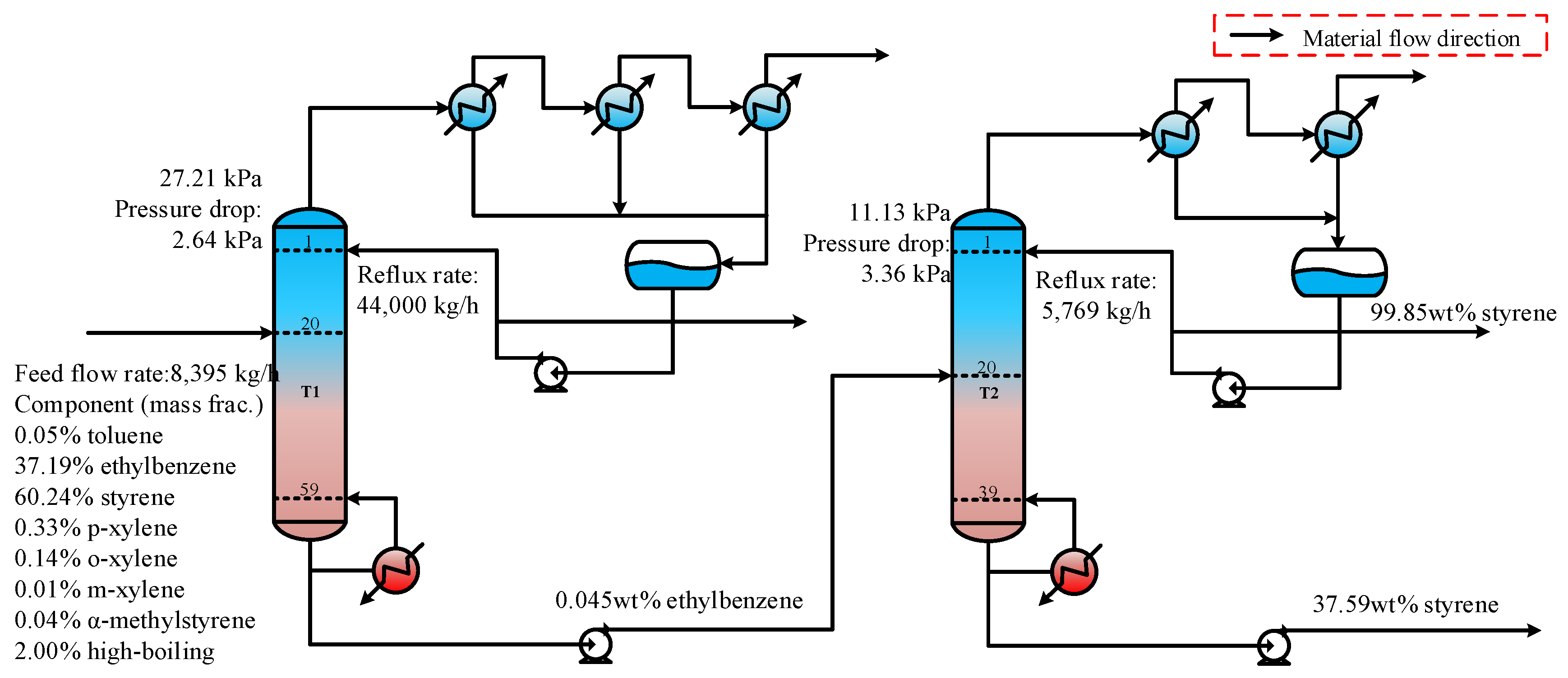
2.1. General Process for Separating the Ethylbenzene–Styrene Mixture
2.2. Dynamic Optimization Problem
3. Optimization Model
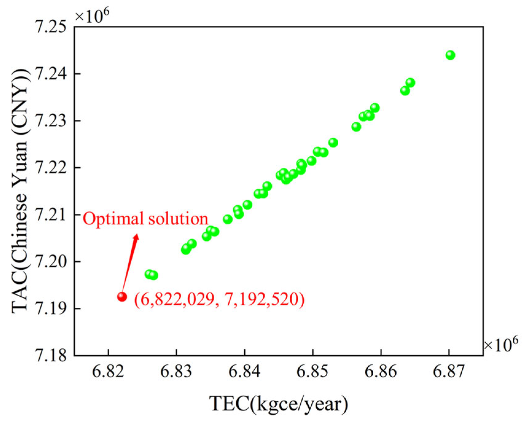
3.1. Steady-State Optimization
3.2. Dynamic Control and Optimization
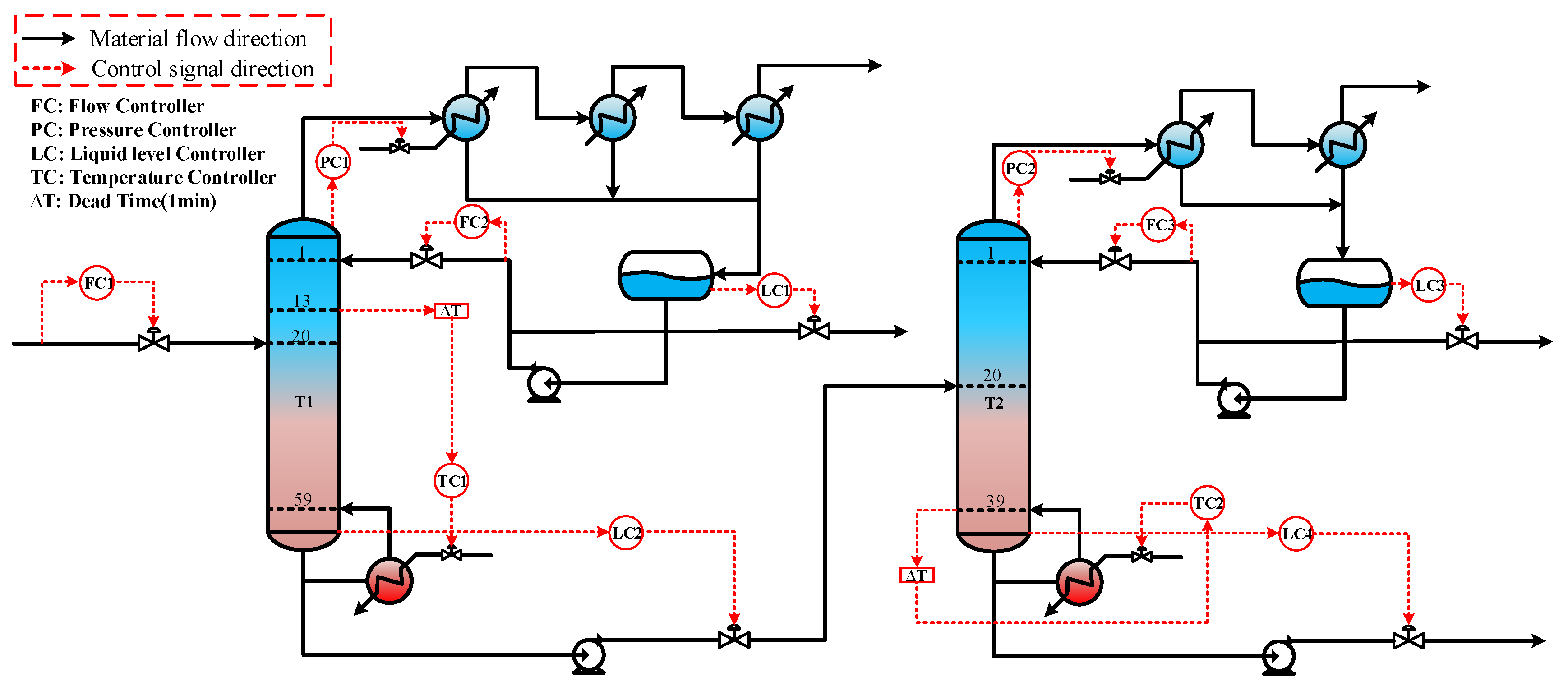
3.2.1. Establishment of Dynamic Control Structure
3.2.2. Performance of Dynamic Control
3.2.3. Dynamic Optimization Model
4. Results and Discussion
4.1. Steady-State Optimization Results
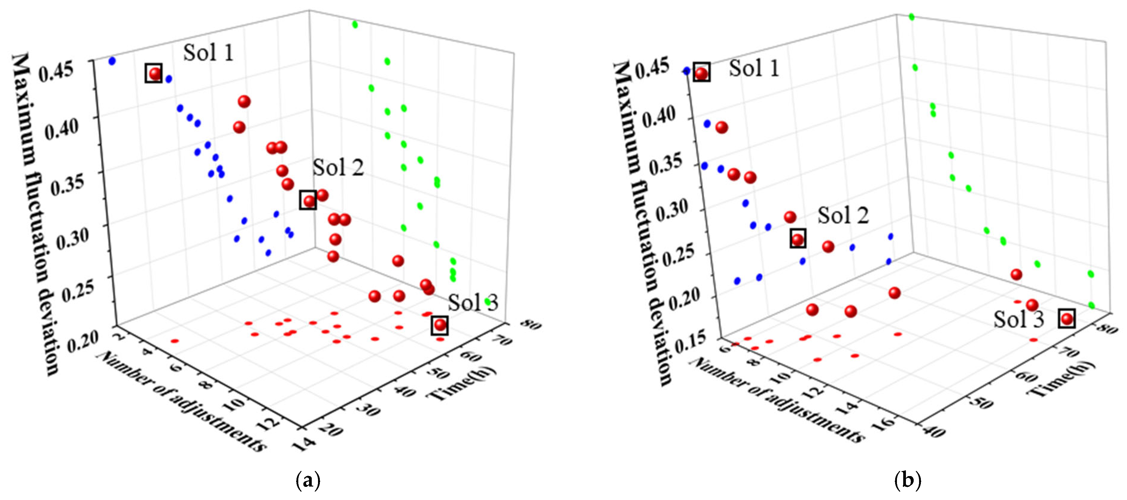
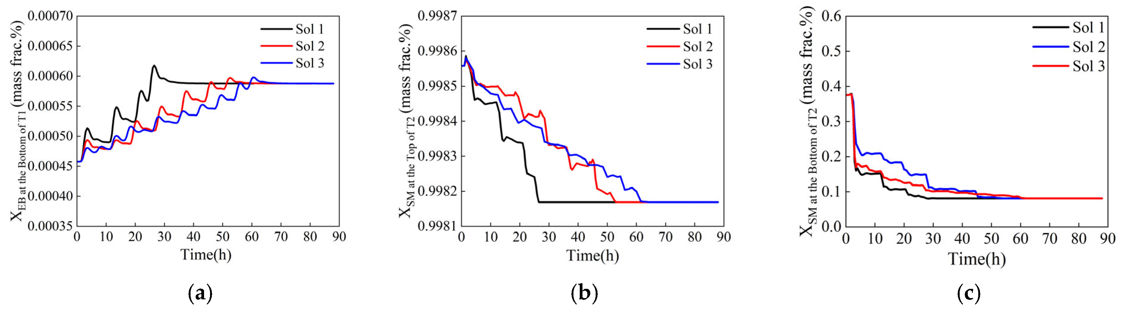
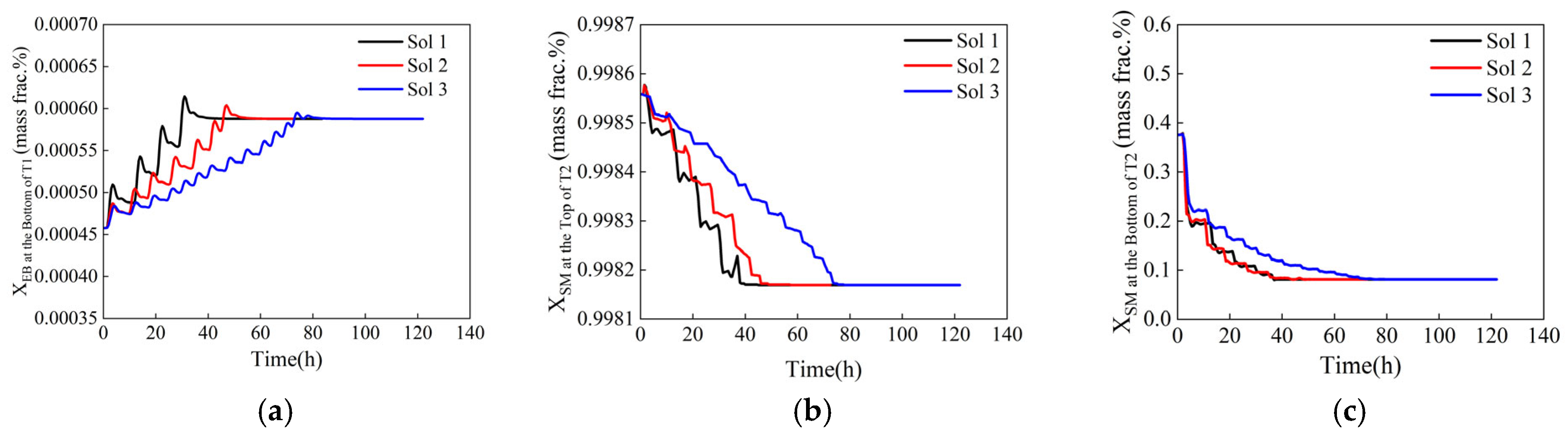
4.2. Dynamic Optimization Results
5. Conclusions
Author Contributions
Funding
Data Availability Statement
Conflicts of Interest
Nomenclature and Abbreviations
| Nomenclature | |
| A | Maximum fluctuation amplitude |
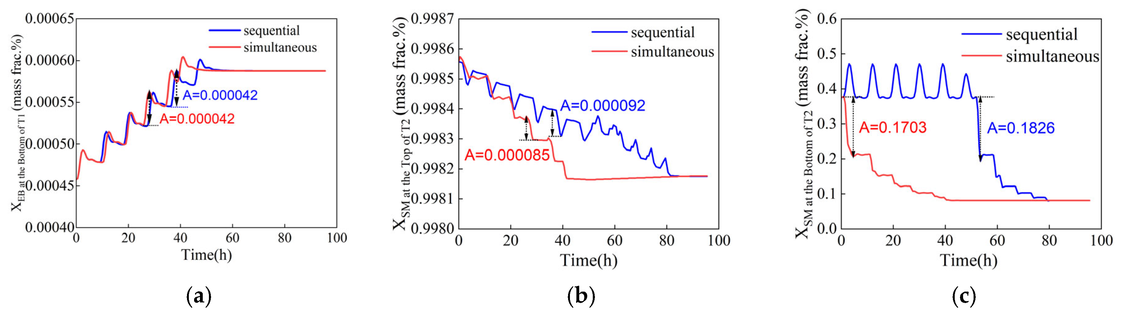
| A(1), A(2) | The maximum fluctuation amplitude of the mass fraction of ethylbenzene at the bottom of T1 and T2 |
| cH2O | Specific heat capacity of water, kJ/(kg·°C) |
| CCW | Prices of cooling water, CNY/t |
| CRW | Prices of chilled water, CNY/t |
| Csteam | Prices of steam, CNY/t |
| gbest | Optimal position of the entire particle swarm |
| Kc | Gain constant |
| L1, L2 | The reflux rates of T1 and T2, kg/h |
| n | The number of adjustment steps |
| pbest | Optimal position of the particles |
| PP | Payback period, year |
| QCW | Duty of condensers cooled by cooling water, kW |
| QR | Reboiler duty, kW |
| QRW | Duty of condensers cooled by chilled water, kW |
| r | The latent heat of vaporization of water vapor, kJ/kg |
| S1, S2 | Step vectors of the reflux flow rates of columns T1 and T2 |
| t | The time of system fluctuation, h |
| αelec | Standard coal equivalent coefficient for electricity, kgce/(kWh) |
| αH2O | Standard coal equivalent coefficients for cooling water, kgce/t |
| αsteam | Standard coal equivalent coefficients for steam, kgce/t |
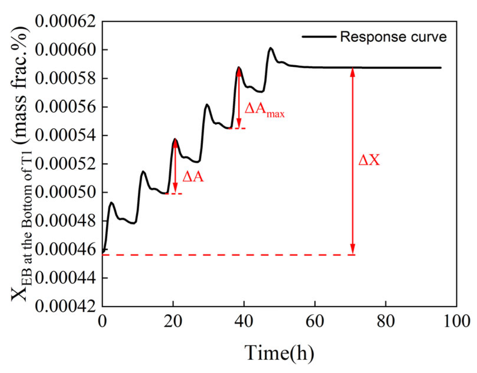
| ΔA | The difference between the maximum and minimum values of mass fraction in each adjustment step |
| ΔTCW | Difference between the supply and return temperatures of cooling water, °C |
| ΔTRW | Difference between the supply and return temperatures of chilled water, °C |
| ΔX | The variation in mass fraction when the reflux flow rate is adjusted from the initial value to the optimal value |
| τ1 | Integration time, min |
| Abbreviations | |
| ce | Coal equivalent |
| CAGR | Compound annual growth rate |
| CNY | Chinese Yuan |
| GA | Genetic algorithm |
| MINLP | Mixed integer nonlinear programming problem |
| MOPSO | Multi-objective particle swarm optimization |
| OP | Output |
| PID | Proportional integral derivative |
| PSO | Particle swarm optimization |
| PV | Process variable |
| SP | Setpoint |
| TAC | Total annualized cost |
| TCI | Total investment cost |
| TEC | Total energy consumption |
| TOC | Total operating cost |
References
- Research and Markets. Styrene Global Market Report 2023. Available online: https://www.researchandmarkets.com/reports/5733831/styrene-global-market-report (accessed on 14 January 2025).
- Zhu, X.; Gao, Y.; Wang, X.; Haribal, V.; Liu, J.; Neal, L.M.; Bao, Z.; Wu, Z.; Wang, H.; Li, F. A Tailored Multi-Functional Catalyst for Ultra-Efficient Styrene Production under a Cyclic Redox Scheme. Nat. Commun. 2021, 12, 1329. [Google Scholar] [CrossRef] [PubMed]
- Li, X.; Cui, C.; Li, H.; Gao, X. Process Synthesis and Simulation-Based Optimization of Ethylbenzene/Styrene Separation Using Double-Effect Heat Integration and Self-Heat Recuperation Technology: A Techno-Economic Analysis. Sep. Purif. Technol. 2019, 228, 115760. [Google Scholar] [CrossRef]
- Jongmans, M.T.G.; Hermens, E.; Raijmakers, M.; Maassen, J.I.W.; Schuur, B.; De Haan, A.B. Conceptual Process Design of Extractive Distillation Processes for Ethylbenzene/Styrene Separation. Chem. Eng. Res. Des. 2012, 90, 2086–2100. [Google Scholar] [CrossRef]
- Muhammed, T. Optimized Energy Efficient Reactive Distillation for Octane Upgrading with Economic and Environmental Considerations. Fuel 2024, 378, 132994. [Google Scholar] [CrossRef]
- Amooey, A.A. Optimization of Operating Parameters for Furfuryl Alcohol Production in a Reactive Distillation Column Using Response Surface Methodology. Results Chem. 2024, 12, 101873. [Google Scholar] [CrossRef]
- Wang, Q.; Zhang, B.J.; He, C.; Chen, Q.L. Simultaneous Optimization of Solvent Composition and Operation Parameters for Sulfolane Aromatic Extractive Distillation Processes. In Proceedings of the 13th International Symposium on Process Systems Engineering—PSE 2018, San Diego, CA, USA, 1–5 July 2018; Eden, M.R., Ierapetritou, M., Towler, G.P., Eds.; Elsevier: San Diego, CA, USA, 2018; Volume 44, pp. 1111–1116. [Google Scholar]
- Yang, A.; Ernawati, L.; Wang, M.; Kong, Z.Y.; Sunarso, J.; Sun, S.; Shen, W. Multi-Objective Optimization of the Intensified Extractive Distillation with Side-Reboiler for the Recovery of Ethyl Acetate and Methanol from Wastewater. Sep. Purif. Technol. 2023, 310, 123131. [Google Scholar] [CrossRef]
- Wang, Y.; Wang, S.; Shan, B.; Ma, Y.; Xu, Q.; Wang, Y.; Cui, P.; Zhang, F. Sustainable Process Design and Multi-Objective Optimization of Efficient and Energy-Saving Separation of Xylene Isomers via Extractive Distillation Based on Double Extractants. Sep. Purif. Technol. 2025, 354, 128899. [Google Scholar] [CrossRef]
- Chandra, P.; Mudgal, A.; Patel, J.; Patel, V.K. Thermo-Economical Modeling and Multi-Objective Optimization of Thermal Energy Driven Multiple Effect Distillation System for Water Treatment Using NSGA-II Algorithm. Desalination Water Treat. 2024, 320, 100646. [Google Scholar] [CrossRef]
- Su, X.-R.; Kusuma, A.A.N.A.N.; Gunawan, J.E.; Haidar, R.; Adhi, T.P.; Adi, V.S.K. Flexible Design and Optimization of Electronic-Grade Propylene Glycol Monomethyl Ether Acetate Production via Integrated Reactive and Pressure-Swing Distillation. Sep. Purif. Technol. 2025, 358, 130440. [Google Scholar] [CrossRef]
- Wang, K.; Xin, L.; Zhang, Y.; Qi, J.; Zhu, Z.; Wang, Y.; Zhong, L.; Cui, P. Sustainable and Efficient Process Design for Wastewater Recovery of Cyclohexane/Isopropyl Alcohol Azeotrope by Extractive Distillation Based on Multi-Objective Genetic Algorithm Optimization. Chem. Eng. Res. Des. 2024, 201, 593–602. [Google Scholar] [CrossRef]
- Wang, S.; Wang, Y.; Sun, K.; Xu, Q.; Wang, Y.; Zhang, F.; Shan, B. Sustainable and Efficient-Saving Process Synthesis Design for Separating Methanol-Water-Toluene via Extractive Distillation Based on Multi-Objective Optimization. Process Saf. Environ. Prot. 2024, 190, 262–276. [Google Scholar] [CrossRef]
- Yin, T.; Zhang, Q.; Chen, Y.; Liu, C.; Xiang, W. Process Design and Optimization of the Reactive-Extractive Distillation Process Assisted with Reaction Heat Recovery via Side Vapor Recompression for the Separation of Water-Containing Ternary Azeotropic Mixture. Process Saf. Environ. Prot. 2024, 184, 1041–1056. [Google Scholar] [CrossRef]
- Murrieta-Dueñas, R.; Cortez-González, J.; Segovia-Hernández, J.G.; Hernández-Aguirre, A.; Gutiérrez-Guerra, R.; Hernández, S. A Comparative Analysis of Differential Evolution and Boltzmann-Based Distribution Algorithms with Constraint Handling Techniques for Distillation Process Optimization. Chem. Eng. Res. Des. 2025, 214, 39–53. [Google Scholar] [CrossRef]
- Leng, J.; Fan, S.; Dong, L.; Feng, Z. Design and Optimization of Energy-Saving Heterogeneous Azeotropic Distillation Processes for the Separation of Ternary Mixture of Ethyl Acetate/n-Propanol/Water. Sep. Purif. Technol. 2025, 359, 130537. [Google Scholar] [CrossRef]
- Li, M.; Peng, J.; Cheng, Y.; Zhang, Z.; Ma, Y.; Gao, J. Dual-Objective Optimization and Energy Efficiency Enhancement of Natural Decantation Assisted Extractive Distillation Process for n-Butanol/Isobutanol/Water Separation. Sep. Purif. Technol. 2024, 336, 126336. [Google Scholar] [CrossRef]
- Tian, X.; Wang, R.; Wang, H.; Li, C.; Liu, J. Energy-Saving Extractive Distillation Processes Design and Optimization for the Separation of Ethyl Acetate and n-Heptane Azeotrope. Fuel 2025, 379, 132974. [Google Scholar] [CrossRef]
- Li, S.; Zheng, Y.; Li, S.; Huang, M. Mechanism-Embedded Neural Network Modeling and Operation Optimization of a Distillation Unit with Varying Production Performance. Chem. Eng. Res. Des. 2022, 183, 221–234. [Google Scholar] [CrossRef]
- Li, S.; Zheng, Y.; Zou, Y.; Li, S. Enhancing Interactive Optimization with Operating Condition Supervision for Distillation Units. Control Eng. Pract. 2024, 148, 105942. [Google Scholar] [CrossRef]
- Wang, Z.; Zhang, H.; Liu, D. Dynamic Optimization for SP of Control Loops Using Adaptive APC Techniques. J. Taiwan Inst. Chem. Eng. 2025, 167, 105858. [Google Scholar] [CrossRef]
- Shin, Y.; Smith, R.; Hwang, S. Development of Model Predictive Control System Using an Artificial Neural Network: A Case Study with a Distillation Column. J. Clean. Prod. 2020, 277, 124124. [Google Scholar] [CrossRef]
- Huang, D.; Luo, X.-L. Process Transition Based on Dynamic Optimization with the Case of a Throughput-Fluctuating Ethylene Column. Ind. Eng. Chem. Res. 2018, 57, 6292–6302. [Google Scholar] [CrossRef]
- Zhang, Y.; Mo, Y. Dynamic Optimization of Chemical Processes Based on Modified Sailfish Optimizer Combined with an Equal Division Method. Processes 2021, 9, 1806. [Google Scholar] [CrossRef]
- Haider, P.; Freko, P.; Lochner, S.; Reiter, T.; Rehfeldt, S.; Klein, H. Design of a Test Rig for the Simulation of Startup Procedures in Main Heat Exchangers of Air Separation Plants. Chem. Eng. Res. Des. 2019, 147, 90–97. [Google Scholar] [CrossRef]
- Aucejo, A.; Loras, S.; Martínez-Soria, V.; Becht, N.; Del Río, G. Isobaric Vapor−Liquid Equilibria for the Binary Mixtures of Styrene with Ethylbenzene, o-Xylene, m-Xylene, and p-Xylene. J. Chem. Eng. Data 2006, 51, 1051–1055. [Google Scholar] [CrossRef]
- Song, Z.; Cui, W.; Wu, Y.; Wu, B.; Chen, K.; Ji, L. Energy, Exergy, Economic, and Environmental Analysis of a Novel Liquid-Only Transfer Dividing Wall Column with Vapor Recompression. Sep. Purif. Technol. 2024, 329, 125122. [Google Scholar] [CrossRef]
- Parhi, S.S.; Rangaiah, G.P.; Jana, A.K. Multi-Objective Optimization of Vapor Recompressed Distillation Column in Batch Processing: Improving Energy and Cost Savings. Appl. Therm. Eng. 2019, 150, 1273–1296. [Google Scholar] [CrossRef]
- Tang, Y.; Long, W.; Wang, Y.; Xiao, G.; Wang, Y.; Lu, M. Multi-Objective Optimization of Methanol Reforming Reactor Performance Based on Response Surface Methodology and Multi-Objective Particle Swarm Optimization Coupling Algorithm for on-Line Hydrogen Production. Energy Convers. Manag. 2024, 307, 118377. [Google Scholar] [CrossRef]
- Wang, D.; Tan, D.; Liu, L. Particle Swarm Optimization Algorithm: An Overview. Soft Comput. 2018, 22, 387–408. [Google Scholar] [CrossRef]
- Cui, Y.; Geng, Z.; Zhu, Q.; Han, Y. Review: Multi-Objective Optimization Methods and Application in Energy Saving. Energy 2017, 125, 681–704. [Google Scholar] [CrossRef]
- Geng, X.; Xu, D.; Hou, Z.; Li, H.; Gao, X. Novel Dynamic Control Structure of Reactive Distillation Process for Isopropanol Production via Transesterification. Chem. Eng. Res. Des. 2024, 205, 131–147. [Google Scholar] [CrossRef]
- Luyben, W.L. Principles and Case Studies of Simultaneous Design; John Wiley & Sons, Inc.: Hoboken, NJ, USA, 2011; ISBN 978-0-470-92708-3. [Google Scholar]
- Shan, B.; Niu, C.; Meng, D.; Zhao, Q.; Ma, Y.; Wang, Y.; Zhang, F.; Zhu, Z. Control of the Azeotropic Distillation Process for Separation of Acetonitrile and Water with and without Heat Integration. Chem. Eng. Process.—Process Intensif. 2021, 165, 108451. [Google Scholar] [CrossRef]
- Luyben, W.L. Control of a Three-Column Distillation Process for Separating Acetonitrile, Chloroform and Ethanol. Sep. Purif. Technol. 2025, 360, 131081. [Google Scholar] [CrossRef]
- Luyben, W.L. Distillation Design and Control Using AspenTM Simulation; John Wiley & Sons, Inc.: Hoboken, NJ, USA, 2013; ISBN 978-1-118-41143-8. [Google Scholar]
- Luyben, W.L. Tuning Proportional−Integral−Derivative Controllers for Integrator/Deadtime Processes. Ind. Eng. Chem. Res. 1996, 35, 3480–3483. [Google Scholar] [CrossRef]
- Shan, B.; Sun, D.; Zheng, Q.; Zhang, F.; Wang, Y.; Zhu, Z. Dynamic Control of the Pressure-Swing Distillation Process for THF/Ethanol/Water Separation with and without Thermal Integration. Sep. Purif. Technol. 2021, 268, 118686. [Google Scholar] [CrossRef]
- Luyben, W.L. Design and Control of a Pressure-Swing Distillation Process with Vapor Recompression. Chem. Eng. Process.—Process Intensif. 2018, 123, 174–184. [Google Scholar] [CrossRef]
- Dai, Y.; Xu, Y.; Wang, S.; Li, S.; Wang, Y.; Gao, J. Dynamics of Hybrid Processes with Mixed Solvent for Recovering Propylene Glycol Methyl Ether from Wastewater with Different Control Structures. Sep. Purif. Technol. 2019, 229, 115815. [Google Scholar] [CrossRef]
- Bravo Sanchez, F.J.; English, N.B.; Hossain, M.R.; Moore, S.T. Improved Analysis of Deep Bioacoustic Embeddings through Dimensionality Reduction and Interactive Visualisation. Ecol. Inform. 2024, 81, 102593. [Google Scholar] [CrossRef]
- Xiong, H.; Song, J.; Liu, J.; Han, Y. Deep Transfer Learning-Based SSVEP Frequency Domain Decoding Method. Biomed. Signal Process. Control 2024, 89, 105931. [Google Scholar] [CrossRef]


| Controllers | Gain Constant Kc | Integration Time τ1/min | Mode of Acting |
|---|---|---|---|
| Flow Controller | 0.5 | 0.3 | reverse |
| Pressure Controller | 2 | 10 | reverse |
| Liquid Level Controller | 2 | 9999 | direct |
| Temperature Controller (TC1) | 4.5288 | 14.52 | reverse |
| Temperature Controller (TC2) | 2.3692 | 7.92 | reverse |
| Component | Initial Feed Composition | Feed Composition with Disturbance (Mole Fraction) | |
|---|---|---|---|
| +10% Disturbance | −10% Disturbance | ||
| α-Methylstyrene | 0.000343 | 0.000343 | 0.000343 |
| Ethylbenzene | 0.37031 | 0.42031 | 0.32031 |
| High-boiling component | 0.012593 | 0.012593 | 0.012593 |
| M-xylene | 0.001344 | 0.001344 | 0.001344 |
| O-xylene | 0.0001 | 0.0001 | 0.0001 |
| P-xylene | 0.003307 | 0.003307 | 0.003307 |
| Styrene | 0.611467 | 0.561467 | 0.661467 |
| Toluene | 0.000535 | 0.000535 | 0.000535 |
| Method | Solution | Step Length for Adjusting the Reflux Flow of T1 (kg/h) | Step Length for Adjusting the Reflux Flow of T2 (kg/h) |
|---|---|---|---|
| Variable-step optimization | Sol 1 | [768.64, 767.21, 633.30, 678.65] | [1629.37, 1358.93, 1148.67, 619.33] |
| Sol 2 | [510.27, 212.70, 510.27, 510.27, 510.27, 372.73, 221.30] | [830.46, 290.66, 572.57, 1255.70, 290.66, 1225.59, 290.66] | |
| Sol 3 | [331.57, 155.26, 319.92, 331.57, 66.31, 320.80, 250.67, 229.65, 280.24, 331.57, 163.94, 66.31] | [1251.77, 250.35, 531.40, 250.35, 250.35, 719.94, 250.35, 250.35, 250.35, 250.35, 250.35, 250.35] | |
| Equal-step optimization | Sol 1 | [724.38, 724.38, 724.38, 674.65, 0] | [977, 977, 977, 977, 848.3] |
| Sol 2 | [415.22, 415.22, 415.22, 415.22, 415.22, 415.22, 356.49] | [899.67, 899.67, 899.67, 899.67, 899.67, 257.94, 0] | |
| Sol 3 | [200, 200, 200, 200, 200, 200, 200, 200, 200, 200, 200, 200, 200, 200, 47.8] | [358.25, 358.25, 358.25, 358.25, 358.25, 358.25, 358.25, 358.25, 358.25, 358.25, 358.25, 358.25, 358.25, 99.07, 0] |
Disclaimer/Publisher’s Note: The statements, opinions and data contained in all publications are solely those of the individual author(s) and contributor(s) and not of MDPI and/or the editor(s). MDPI and/or the editor(s) disclaim responsibility for any injury to people or property resulting from any ideas, methods, instructions or products referred to in the content. |
© 2025 by the authors. Licensee MDPI, Basel, Switzerland. This article is an open access article distributed under the terms and conditions of the Creative Commons Attribution (CC BY) license (https://creativecommons.org/licenses/by/4.0/).
Share and Cite
Jiang, G.; She, Y.; Song, Z.; Zhao, L.; Liu, G. Optimization and Dynamic Adjustment of Tandem Columns for Separating an Ethylbenzene–Styrene Mixture Using a Multi-Objective Particle Swarm Algorithm. Separations 2025, 12, 161. https://doi.org/10.3390/separations12060161
Jiang G, She Y, Song Z, Zhao L, Liu G. Optimization and Dynamic Adjustment of Tandem Columns for Separating an Ethylbenzene–Styrene Mixture Using a Multi-Objective Particle Swarm Algorithm. Separations. 2025; 12(6):161. https://doi.org/10.3390/separations12060161
Chicago/Turabian StyleJiang, Guangsheng, Yibo She, Zhongwen Song, Liwen Zhao, and Guilian Liu. 2025. "Optimization and Dynamic Adjustment of Tandem Columns for Separating an Ethylbenzene–Styrene Mixture Using a Multi-Objective Particle Swarm Algorithm" Separations 12, no. 6: 161. https://doi.org/10.3390/separations12060161
APA StyleJiang, G., She, Y., Song, Z., Zhao, L., & Liu, G. (2025). Optimization and Dynamic Adjustment of Tandem Columns for Separating an Ethylbenzene–Styrene Mixture Using a Multi-Objective Particle Swarm Algorithm. Separations, 12(6), 161. https://doi.org/10.3390/separations12060161