Development of an Adaptive Model for the Rate of Steel Corrosion in a Recirculating Water System

Abstract

The stable quality of circulating water ensures the long-term stable operation of various processes in petrochemical production and achieves energy savings and emission reduction while reducing environmental pollution and yielding economic benefits to petrochemical enterprises. However, traditional circulating water quality evaluation and modeling for corrosion rate prediction suffer from adaptability and accuracy problems. To address these problems, the water quality analysis data of the circulating water in the field were subjected to data preprocessing and water quality index calculation to perform feature engineering, followed by modeling using a machine learning method that integrates the adaptive immune genetic algorithm and random forest (RF) algorithm and can intelligently select the water quality parameters to be used as the input variables for the RF modeling. Finally, the method was validated using an industrial example, and the results indicate that the method is capable of removing interference variables and is suitable for carbon steel corrosion rate prediction based on water quality models. The proposed method provides a basis for water quality management and real-time decision-making by circulating water field personnel.

1. Introduction

Industrial circulating water is an important processing medium in petrochemical production. Circulating cooling water is continuously recycled through the system and is affected by many factors, such as microorganisms, impurities, the water flow speed, and the equipment environment. Consequently, it can easily cause equipment corrosion, scale deposits, and pipeline blockage, resulting in accidents such as heat exchange inefficiency and leakage, and hence leading to a reduction in production load and product yield and unplanned shutdowns. Therefore, it is important to ensure the stability of the circulating water quality in petrochemical production. Water quality monitoring, especially corrosion rate control, is the main means of water quality management, and it is also the key to maintaining a stable water quality.

Water quality monitoring requires that a corresponding water quality model be established first [1]. The model should be able to comprehensively analyze and evaluate the water quality of the water body according to the values of the water quality parameters (WQPs) and then to characterize the scaling and corrosion of the heat exchange equipment by the circulating water [2]. The term water quality model is a general term referring to mathematical models that comprehensively consider the biochemical reactions and physical effects of the pollutants in the water body and describe the mixing, transport, and transformation of the substances in the water body [3]. Since the concept was proposed in the 1920s, water quality models have developed very rapidly. In the initial development stage, deterministic water quality models, including oxygen balance models [4,5,6], morphological models [7], and comprehensive multi-media models [8,9,10], were mostly studied. Later, with the increasing complexity of water quality models, a multitude of uncertain factors were identified in the water environment. Thus, the established deterministic water quality models fail to accurately characterize the actual water body. Since the 1960s, researchers have studied the uncertainty of water bodies and have developed probabilistic water quality models.

The water quality in a circulating water system used in petrochemical production is affected by many factors. Uncertain water quality models often exhibit high-dimensional, nonlinear, and other characteristics, making it difficult to establish an accurate mathematical model to describe the quality of the circulating water in petrochemical production and for its evaluation and prediction using traditional methods [11]. In recent years, with the development of artificial intelligence and big data technology and the ability of enterprises to store massive production data, the application of intelligent algorithms to nonlinear scientific problems, especially the use of machine learning methods represented by artificial neural networks (ANNs) for water quality modeling, has become a typical direction of research. In terms of water quality parameter (WQP) prediction, Alizadeh and Kavianpour [12] used different combinations of water quality parameters as input variables to predict the daily salinity, temperature, and dissolved oxygen values, as well as the hourly dissolved oxygen values, by comparing the ANN and wavelet neural network (WNN) models. D’Souza and Kumar [13] used an ANN-based data-driven modeling approach to predict the temporal variations in two important indexes of water quality, i.e., the residual chlorine and biomass. Zhu et al. [14] proposed a water quality evaluation model based on a back-propagation neural network (BPNN), which they then optimized via particle swarm optimization. In the characterization of the corrosion rate, Gao et al. [15] used WQPs to establish a corrosion scaling rate prediction model based on a BPNN and compared it with actual analysis data for validation. Li et al. [16,17] analyzed high-concentration, multi-water quality data, and on this basis, selected water quality parameters that have a greater impact on the corrosion rate and adhesion rate. Then, they developed a corrosion rate and adhesion rate prediction model based on a Nonlinear Auto Regressive model with Exogenous Inputs (NARX) neural network and finally established an intelligent auxiliary analysis platform for industrial-circulating cooling water based on their water quality prediction model. Based on experimental data, Yang et al. [18] established an intelligent prediction model for the cooling water corrosion rate based on the least squares support vector machine (LS-SVM), taking the corrosion-related water quality factors as the input variables and the corrosion rate as the output variable. Their results indicate that the LS-SVM model is simpler and has a better generalization ability than the traditional methods. Yang et al. [19] established a NARX neural network prediction model to predict the adhesion rate.

However, the above models do not consider the degree of the impact of the water quality data on the target, and thus, we cannot make full use of their evaluation results based on the ideal state of the water quality. Considering the advantages of water quality index (WQI) methods in the evaluation and monitoring of the water quality of rivers, lakes, and drinking water [20], in this study, the WQIs were used to calculate the water quality analysis data during the data preprocessing and the model feature engineering, and the calculated data were then used as the model’s input. In addition, feature selection is an important step in machine learning modeling, and it has an important impact on the model’s accuracy [21]. However, the formation mechanism of the scaling and corrosion of heat exchangers in industrial circulating cooling water systems is an extremely complex physicochemical process [22], so intelligent algorithms are required to perform the feature selection. According to the different evaluation criteria, the feature selection can be carried out using three methods, i.e., the embedded method, the filter method, and the wrapper method [23,24]. The wrapper method has a high accuracy and retains the physical meaning of the model variables, but the genetic algorithm (GA), which is commonly used in the wrapper method, suffers from premature convergence [25]. To improve the global search capability of the algorithm, the principle of a biological immune mechanism was introduced into the simple GA to construct a new improved GA, i.e., the immune GA (IGA) [26]. Based on the IGA, the adaptive IGA (AIGA) introduces an adaptive search mechanism based on the entropy information in order to control the probabilities in the crossover and mutation operations. This further alleviates the premature convergence problem of the traditional GA [27,28,29], enabling the feature selection to be executed adaptively and efficiently according to the predictability of the subsequent process modeling algorithms, and thereby improving the model’s accuracy. Furthermore, process modeling using the random forest (RF) algorithm, compared to that using traditional machine learning algorithms such as the BPNN and SVR, has a good tolerance for outliers and noise, is not prone to overfitting, and is insensitive to multicollinearity [30,31]. Therefore, in this study, the WQIs were introduced to the preprocessed WQPs, and then, the AIGA-RF machine learning algorithm was used for the water quality modeling in order to predict the corrosion rate of carbon steel. Then, the AIGA was integrated for the wrapper feature selection and the RF was used for the process modeling. The constructed model was found to have a good prediction performance and a good tolerance for outliers and noise.

The rest of this article is organized as follows. Section 2 describes how the water quality data were preprocessed and the WQIs were calculated as the input of the subsequent model, and then, an AIGA-RF water quality model is established to predict the corrosion rate. Section 3 focuses on the validation of the effectiveness of the model through examples, and finally, the major findings are presented.

2. AIGA-RF Water Quality Model Based on WQIs

The WQIs were calculated for the feature engineering in the water quality modeling to obtain better training data features, and then, a water quality modeling method, i.e., the AIGA-RF, was developed based on AIGA feature selection and machine learning to predict the corrosion rate. A flowchart of the methodology is shown in Figure 1.

2.1. Data Preprocessing and WQI Calculation

2.1.1. Data Preprocessing

To ensure the accuracy of the model, first, the water quality analysis data need to be collected and preprocessed, including the removal of invalid data, boxplot analysis of outliers, and linear interpolation and fitted filling of missing data [32].

Water quality analysis data set $X$ can be expressed as an (m × n)-dimensional matrix:

$$X=\left[\begin{array}{cccc}{x}_{1,1}& \cdots & x_{j,1}& \begin{array}{cc}\cdots & x_{m,1}\end{array}\\ ⋮& \ddots & ⋮& \begin{array}{cc}\ddots & ⋮\end{array}\\ x_{1,i}& \cdots & x_{j,i}& \begin{array}{cc}\cdots & x_{m,i}\end{array}\\ \begin{array}{c}⋮\\ x_{1,n}\end{array}& \begin{array}{c}\ddots \\ \cdots \end{array}& \begin{array}{c}⋮\\ x_{j,n}\end{array}& \begin{array}{c}\begin{array}{cc}\ddots & ⋮\end{array}\\ \begin{array}{cc}\cdots & x_{m,n}\end{array}\end{array}\end{array}\right]$$

(1)

where $x_{j,i}$ is the analysis value of the jth WQP in the ith data record, $i=1,2,\cdots n$, and $j=1,2,\cdots m$. Furthermore, m is the number of all of the collected WQPs (features), and n is the number of collected data records.

If all of the WQPs in the ith data record are expressed as a vector $X_i$, then

$$X_i=\left[x_{1,i},\cdots x_{j,i},\cdots ,x_{m,i}\right],$$

(2)

$$X={\left[X_1,\cdots X_i,\cdots ,X_n\right]}^T.$$

(3)

$y_i$ is the actual corrosion rate of the ith data record, and $y$ is the set of $y_i$ in the whole range. Then, the variables predicted by the model can be expressed as a (1 × n)-dimensional matrix:

$$y={\left[y_1,\cdots y_i,\cdots ,y_n\right]}^T.$$

(4)

2.1.2. WQI Calculation

Traditional water quality evaluation methods are based on the comparison between the experimentally determined parameter values and the existing guidelines. These data may not be able to explain the variation in the water quality over time and in different geographic areas, nor do they easily give an overall picture of the spatial and temporal trends of the overall water quality [33]. To solve this problem, attempts have been made to use the WQIs to represent the water quality data [34]. The WQIs quantify the overall situation of the water quality and eliminate the evaluation of the water quality [35,36]. Drawing on the process of constructing WQIs for rivers, lakes, and drinking water [37,38,39], in this study, the WQIs of the WQPs of the circulating water in petrochemical production were calculated. The calculation process was as follows.

The design limits (DLs) and permissible limits (PLs) of the circulating water WQPs were set according to the water quality management regulations and field production experience. The values are listed in

Table 1. Circulating water WQP settings.

Parameter	Design Upper and Lower Limits	Permissible Upper and Lower Limits	Unit	Frequency
pH	8.4–8.5	8.1–8.6	/	3 times/day
Turbidity	<20	<35	mg/L	3 times/day
Residual chlorine	0.5–0.8	0.2–1	mg/L	3 times/day
Potassium ion	<30	<40	mg/L	1 time/day
Calcium hard	400–500	<800	mg/L	1 time/day
Concentration multiple	4–5	3–6	/	1 time/day
Total hardness	600–800	400–1200	mg/L	1 time/day
Conductivity	1000–2000	400–3000	mg/L	1 time/day
Total iron	0.5–0.8	<1	mg/L	1 time/day
Chloride ion	300–400	<500	mg/L	3 times/week
Heterotrophic bacteria	<5000	<10,000	Counts	1 time/week
Suspended matter	10–20	<30	mg/L	1 time/week

. The modified permissible limits (MPLs) were calculated using Equation (5).

$$MPL=0.8\cdot PL+0.2\cdot DL.$$

(5)

Finally, the WQI ${\tilde{x}}_{j,i}$ corresponding to $x_{j,i}$ was calculated as follows.

$$\mathrm{If} x_{j,i}\le DL, \mathrm{then} {\tilde{x}}_{j,i}=0.$$

(6)

$$\mathrm{If} DL<x_{j,i}<MPL, \mathrm{then} {\tilde{x}}_{j,i}=\frac{x_{j,i}-DL}{PL-DL}.$$

(7)

$$\mathrm{If} MPL\le x_{j,i}<PL, \mathrm{then} {\tilde{x}}_{j,i}=2\times \frac{x_{j,i}-DL}{MPL-DL}.$$

(8)

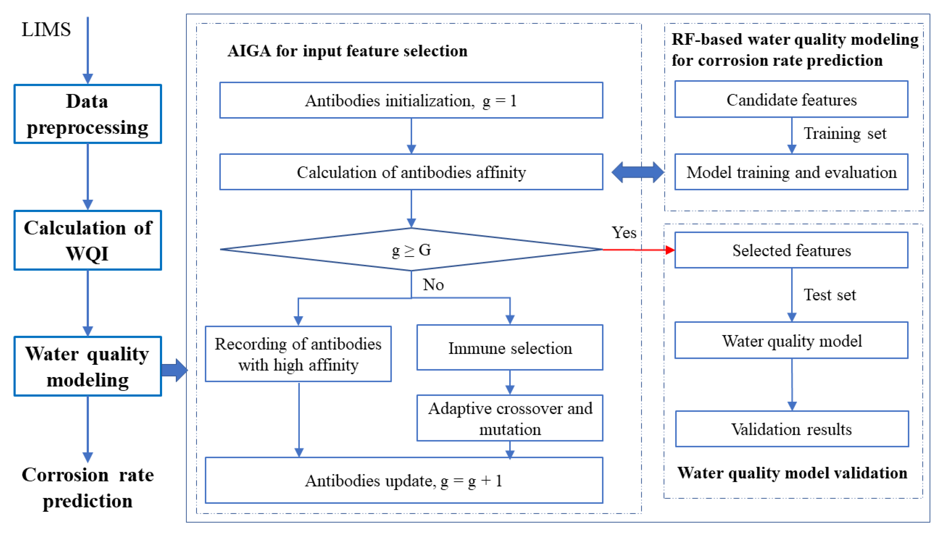
2.2. Corrosion Rate Prediction Using the AIGA-RF Method

Here, the modeling method for predicting the corrosion rate using the AIGA-RF is described in detail. The method includes AIGA-based feature selection of the WQIs and an RF machine learning algorithm for corrosion rate modeling (the steps in the rounded box in Figure 1).

2.2.1. Initialization of Antibodies

A control vector B is introduced in the corrosion rate modeling to control the selection of the process features.

$$B=\left[b_j\right],j=(1,2,\cdots ,m),$$

(9)

where

$$b_j=\{\begin{array}{c}0,exclusion\\ 1,inclusion\end{array}.$$

(10)

In the evolutionary process, $N$ control vectors are randomly generated as the antibody population. Each control vector is considered to be an individual antibody, $B_i$.

2.2.2. Antigen Recognition and Affinity Calculation

After initialization of the antibody population, the corresponding set of input variables for the RF modeling is determined. Subsequently, the WQIs corresponding to the WQPs determined by the antibodies using the RF algorithm are used as input variables to train the corrosion rate prediction model. This process is similar to the recognition of antigens in biological systems. It should be noted that the collected water quality dataset was proportionally divided into two parts, one for model training and the other for model evaluation.

After the model training, each obtained RF model is evaluated. In this study, the mean square error (MSE) was used as an affinity index for each antibody $A_t$ to evaluate the prediction accuracy of the obtained model. The higher the affinity is, the higher the accuracy of the model. The equation for calculating the affinity is

$$A_t=MSE(y_t,y_t^{\prime })=\frac{1}{T}{\displaystyle {\sum }_{t=1}^T{(y_t-y_t^{\prime })}^2},$$

(11)

where $y_t$ is the actual value, corresponding to the tth antibody; $y_t^{\prime }$ is the output of the RF model, corresponding to the tth antibody; and $T$ is the number of antibodies.

2.2.3. Evaluation of Termination Conditions

The antibody production information is used to determine the termination of the feature selection optimization process. If the number of evolutionary generations, G, is met, then the evolution is exited; otherwise, the process proceeds to the next step. G is determined when the average affinity difference between two iterations is less than 10⁻⁴.

$$G=g+1,$$

(12)

$$s. t. {\overline{A}}_{g+1}-{\overline{A}}_g<{10}^{-4},$$

(13)

where ${\overline{A}}_{g+1}$ and ${\overline{A}}_g$ are the average affinities of the (g+1)th and gth generations, respectively.

2.2.4. Identification of Effective Antibodies

These effective antibodies were identified as the evolutionary basis for the next generation. First, a large number of antibodies with high affinities are recorded. Then, the parent antibodies of the next generation are selected according to the reproduction probability, with the criteria being the affinity and concentration of the antibodies. In the biological immune system, high-affinity and low-concentration antibodies [40] are encouraged to ensure parental diversity and immune balance. Then, adaptive crossover and mutation [29] are applied to the newly generated antibodies, which together with the recorded antibodies, form a new generation.

The goal of the entire evolutionary process is to obtain the model with the most accurate prediction performance. In this process, the most important step is selecting the optimal control vector, B, which minimizes the MSE of the obtained RF model. This problem can be described as follows:

$$B^{*}=\arg \underset{B}{\min }MSE(y_t,y_t^{\prime }).$$

(14)

2.2.5. Validation of the Obtained Corrosion Rate Prediction Model

After the evolution of G generations, the best antibody, B*, is obtained. Specifically, the corrosion rate prediction model with the input WQP features of the optimized model is obtained. Then, validation was performed using the test set.

3. Case Study of the AIGA-RF Water Quality Model

The corrosion rate prediction modeling and industrial validation were carried out based on circulating water quality data from a petrochemical enterprise power plant in northwestern China. The laboratory information management system (LIMS) circulating water quality analysis data were collected from 19 water fields from August 2018 to August 2020, and 12 WQPs closely related to the corrosion rate were selected for subsequent treatment: pH, turbidity, residual chlorine, potassium ion, calcium hardness, multiple concentration, total hardness, conductivity, total iron, chloride ion, heterotrophic bacteria, and suspended matter. For the same factors, different materials have different corrosion rates. Therefore, in order to unify the benchmark, the corrosion coupon material we selected was carbon steel. The analysis frequency for the corrosion rate was 1 time/month, and the other WQPs were divided into four categories in terms of analysis frequency, including 3 times/day, 1 time/day, 3 times/week, and 1 time/week. Then, the $DL$ and $PL$ were set as described in Table 1.

After the data preprocessing and WQI calculations, the time dimension attributes of the WQI and the corrosion rate were unified on a monthly basis by summing the WQIs of the current month according to the analysis frequency, finally yielding 271 datasets for subsequent modeling. In the modeling, the dataset was randomly divided using a ratio of 8:2 to obtain a 12 × 216 training data matrix and a 12 × 55 test data matrix. Finally, AIGA-RF modeling was performed. The model parameters were set described in

Table 2. AIGA-RF model parameter settings.

#	Model Parameter	Value
1	Antibody population size	60
2	Memory capacity	6
3	Number of parameters (variables)	12
4	Diversity evaluation parameter	0.95
5	Number of decision trees in RF	10
6	Maximum number of iterations	8

. An algorithm programmed in Python using the PyTorch framework was run in the JetBrains PyCharm 2019.3.3 x64 environment on a computer configured as follows: Intel(R) Core (TM) i7-7700K CPU @ 4.20 GHz with 8 GB RAM, Windows10.

To evaluate the model’s accuracy, the MSE and mean absolute percentage error (MAPE) were used as the model evaluation indexes, which were calculated using the following equations:

$$MSE=\frac{1}{N}{\displaystyle \sum _{i=1}^N{(y_i^{\prime }-y_i)}^2},$$

(15)

$$MAPE=\frac{1}{N}{\displaystyle \sum _{i=1}^N\left|\frac{y_i^{\prime }-y_i}{y_i}\right|},$$

(16)

where $y_i$ is the actual value, $y_i^{\prime }$ is the predicted value, and $N$ is the number of samples in the test set.

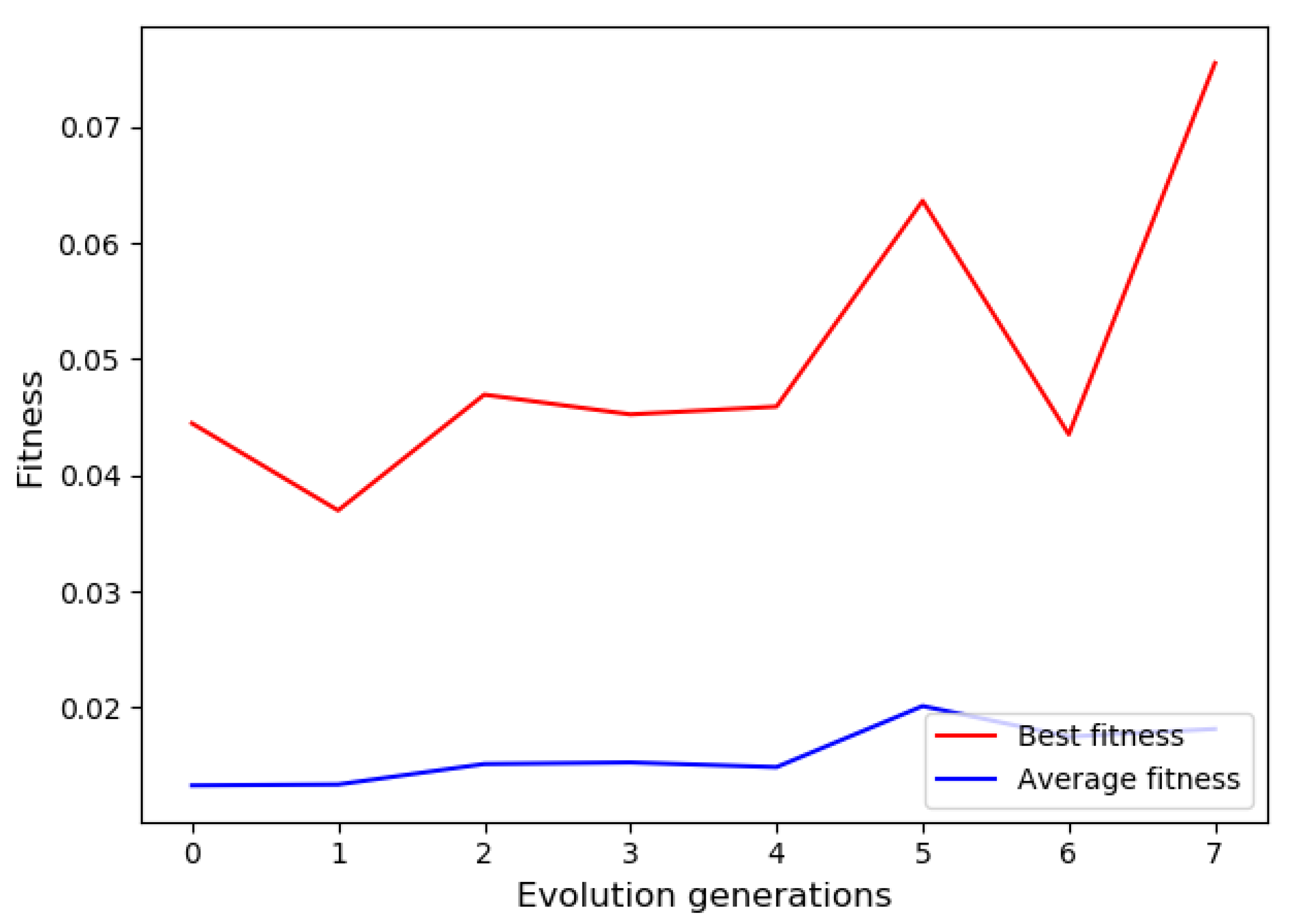
3.1. Feature Selection Using the Optimal Fitted Model and Validation of the Prediction Results

In the case study, the AIGA-based feature selection method was used to select the WQPs so that the most relevant influencing factors in the corrosion prediction model were automatically selected, thus achieving a high model prediction accuracy. Figure 2 shows the convergence of the corrosion rate prediction accuracy target. During the evolutionary process, both the general antibody population and the best antibody candidate population decreased in terms of affinity assessment in the first and sixth generations, while the two exhibited a steady increase in all of the other generations. However, the general antibody population exhibited a gentle performance, while the best antibody candidate population exhibited large fluctuations.

As was described in Section 2.2, the feature selection optimization process is associated with the model training process. That is, the determination of the best feature set indicates the completion of the model fitting. The obtained training model was then validated using the test dataset. The predicted values obtained using the obtained model and the actual production data are compared in Figure 3. It can be seen that the prediction results are closely distributed along the diagonal line, demonstrating a good agreement with the actual values. In this case study, the WQPs selected using the AIGA-RF method were potassium ions, conductivity, total iron, and heterotrophic bacteria. Therefore, these four WQIs should be monitored as a priority to better control the corrosion rate.

3.2. Comparison with Other Modeling Methods

Several other process feature selection methods, including principal component analysis (PCA), GA [41], and IGA [26], and process modeling methods, such as the BPNN and SVR, were also used in this study for comparison. The results are shown in

Table 3. Model comparisons based on MSE and MAPE.

Model	Number of Features	MSE	MAPE
AIGA-RF	4	0.000127	0.31997
AIGA-BP	5	0.000222	0.41478
AIGA-SVR	5	0.000154	0.79707
IGA-RF	8	0.000195	0.32173
GA-RF	5	0.000207	0.57074
PCA-RF	8	0.000467	0.81747
RF	12	0.000405	0.65352

. The proposed AIGA-RF method outperformed the other methods in terms of the model accuracy which is represented by the MSE and MAPE. The comparison of the first three rows shows that the RF modeling has a higher model accuracy. In terms of the feature selection methods, it can be concluded from rows 1, 4, 5, and 6 that the WQPs selected using the AIGA have high correlations with the corrosion rate, reducing the interference of redundant or even irrelevant factors, and thus providing better corrosion rate prediction results.

4. Conclusions

Water quality modeling and corrosion rate prediction are of great importance for monitoring the circulating water quality and maintaining stable water quality in petrochemical enterprises. However, the water quality of the circulating water system in petrochemical enterprises is affected by a multitude of factors, and water quality models often exhibit high-dimensional, nonlinear, and nondeterministic characteristics. Therefore, it is difficult to establish an accurate mathematical model to describe the quality of circulating water in petrochemical enterprises using traditional evaluation and prediction methods. In the present study, the WQIs were calculated based on the WQPs and were used as the inputs of the model. Then, a machine learning-based corrosion rate prediction modeling method was adopted, which employs the AIGA feature selection strategy to automatically select the most suitable WQPs for modeling, and the RF method was used for the water quality modeling. Taking the power plant of a petrochemical enterprise in northwestern China as an example, the corrosion rate of carbon steel was predicted using two years of analysis data for 12 LIMS WQPs from 19 water fields. The results of the case study demonstrate the applicability and effectiveness of the model. A comparison with six other modeling methods (AIGA-BP, AIGA-SVR, IGA-RF, GA-RF, PCA-RF, and RF) revealed that the AIGA can capture the system features better under different modeling situations, thereby improving the accuracy of the model prediction. Therefore, the development of a water quality model for corrosion rate prediction using the AIGA-RF method and using calculated WQI values as the model inputs could be adopted by production enterprises to evaluate the circulating water quality and thus to monitor and control the water quality in real-time.

References

1. Chen, Z.B.; Zhang, H.; Liao, M.X. Integration Multi-Model to Evaluate the Impact of Surface Water Quality on City Sustainability: A Case from Maanshan City in China. Processes 2019, 7, 25. [Google Scholar] [CrossRef] [Green Version]
2. Roberge, P.R.; Sastri, V.S. On-Line Corrosion Monitoring with Electrochemical Impedance Spectroscopy. Corrosion 1994, 50, 744–754. [Google Scholar] [CrossRef]
3. Hahn, H.H.; Schreiner, H. Water-Quality Modeling. Prog. Water Technol. 1978, 10, 185–201. [Google Scholar]
4. Peng, H.; Wang, Y.; Zhang, W.; Li, Y.; Wu, K.B.; Zhu, Q. A Coupled Water Quality-Quantity Model for Water Resource Allocation. In Proceedings of the 2009 3rd International Conference on Bioinformatics and Biomedical Engineering, Beijing, China, 11–13 June 2009; pp. 1–5. [Google Scholar]
5. Shu, S.; Liu, S.; Zhang, D. Water Quality Model Calibration of Water Distribution Network Using Parallel fmGA Algorithm. In Proceedings of the 2010 International Conference on Electrical and Control Engineering, Wuhan, China, 25–27 June 2010; pp. 5801–5804. [Google Scholar]
6. Phelps, E.B.; Streeter, H.W. A Study of the Pollution and Natural Purification of the Ohio River; United States Public Health Service: Washington, DC, USA, 1958. [Google Scholar]
7. Yang, Y.; Wang, Y.; Zhang, W. Numerical Study of Coupled One-Dimensional and Two-Dimensional Hydrodynamic and Water Quality Model for Complex Lake and River Network Areas. In Proceedings of the 2012 International Symposium on Geomatics for Integrated Water Resource Management, Lanzhou, China, 19–21 October 2012; pp. 1–5. [Google Scholar]
8. Pozdnyakov, D.V.; Lyaskovsky, A.V.; Tanis, F.J.; Lyzenga, D.R. Modeling of apparent hydro-optical properties and retrievals of water quality in the Great Lakes for SeaWiFS: A comparison with in situ measurements. In Proceedings of the IEEE 1999 International Geoscience and Remote Sensing Symposium. IGARSS’99 (Cat. No.99CH36293), Hamburg, Germany, 28 June–2 July 1999; Volume 5, pp. 2742–2744. [Google Scholar]
9. Moustafa, K.A.F.; Gaafar, M.Y.; Abuelyazid, T. Modeling and Identification of A Stochastic Water-Quality System Using Actual Data. IEEE Proc. D Control Theory Appl. 1986, 133, 159–164. [Google Scholar] [CrossRef]
10. Powers, W.F.; Canale, R.P. Some Applications of Optimization Techniques to Water-Quality Modeling and Control. IEEE Trans. Syst. Man Cybern. 1975, SMC5, 312–321. [Google Scholar] [CrossRef]
11. Kaji, A.; Taheriyoun, M.; Taebi, A.; Nazari-Sharabian, M. Comparison and optimization of the performance of natural-based non-conventional coagulants in a water treatment plant. J. Water Supply Res. Technol. Aqua 2020, 69, 28–38. [Google Scholar] [CrossRef]
12. Alizadeh, M.J.; Kavianpour, M.R. Development of wavelet-ANN models to predict water quality parameters in Hilo Bay, Pacific Ocean. Mar. Pollut. Bull. 2015, 98, 171–178. [Google Scholar] [CrossRef]
13. D’Souza, C.D.; Kumar, M.S.M. Comparison of ANN models for predicting water quality in distribution systems. J. Am. Water Work. Assoc. 2010, 102, 92–106. [Google Scholar] [CrossRef]
14. Zhu, C.; Zhao, X.; Zhou, J. ANN based on PSO for Surface Water Quality Evaluation Model and Its Application. In Proceedings of the 2009 Chinese Control and Decision Conference, Guilin, China, 17–19 June 2009; pp. 3264–3268. [Google Scholar]
15. Gao, Q.; Ma, T.; Li, J.; Li, C. The research of the water quality prediction model for the circulating cooling water system. Appl. Mech. Mater. 2013, 385, 408–411. [Google Scholar] [CrossRef]
16. Li, J.; Wang, T.; Zhao, Y.; Yang, J.; Gao, Q. Intelligent Analysis Platform of Industrial Circulating Water Based on VB and Matlab. In Proceedings of the 2015 IEEE International Conference on Mechatronics and Automation (ICMA), Beijing, China, 2–5 August 2015; pp. 654–658. [Google Scholar]
17. Wang, T.; Li, J.; Liu, M.; Gao, Q.; Yang, J. Design and Implementation of Intelligent Decision-Making System Software for Industrial Circulating Cooling Water. In Proceedings of the 2016 IEEE International Conference on Mechatronics and Automation, Harbin, China, 7–10 August 2016; pp. 73–77. [Google Scholar]
18. Yang, S.; Liu, X.; Cao, S.; Zhao, B.; Hu, Y.; Liu, F.; Men, H.; Xu, Z. Forecasting Corrosion Rate of Cooling Water Based on Least Squares Support Vector Machine. In Proceedings of the 2010 Fourth International Conference on Genetic and Evolutionary Computing, Shenzhen, China, 13–15 December 2010; pp. 833–836. [Google Scholar]
19. Yang, Z.; Junfang, L.; Qiang, G. The Predication of the Adhesion Rate Based on NARX Model. Appl. Mech. Mater. 2014, 687, 1346–1349. [Google Scholar]
20. Radwan, M. Evaluation of Different Water Quality Parameters for the Nile River and the Different Drains. In Proceedings of the 9th International Water Technology Conference, Sharm El-Sheikh, Egypt, 17–20 March 2005; Available online: http://citeseerx.ist.psu.edu/viewdoc/summary?doi=10.1.1.302.1775 (accessed on 10 August 2021).
21. Chandrashekar, G.; Sahin, F. A survey on feature selection methods. Comput. Electr. Eng. 2014, 40, 16–28. [Google Scholar] [CrossRef]
22. Somerscales, E.F.C. Two-Phase Flow Heat Exchangers: Thermal-Hydraulic Fundamentals and Design; Kakaç, S., Bergles, A.E., Fernandes, E.O., Eds.; Springer: Dordrecht, The Netherlands, 1988; pp. 407–460. [Google Scholar]
23. Zhang, R.; Nie, F.; Li, X.; Wei, X. Feature selection with multi-view data: A survey. Inf. Fusion 2019, 50, 158–167. [Google Scholar] [CrossRef]
24. Lee, C.Y.; Wen, M.S. Establish Induction Motor Fault Diagnosis System Based on Feature Selection Approaches with MRA. Processes 2020, 8, 1055. [Google Scholar] [CrossRef]
25. Tran, H.K.; Son, H.H.; Duc, P.V.; Trang, T.T.; Nguyen, H.N. Improved Genetic Algorithm Tuning Controller Design for Autonomous Hovercraft. Processes 2020, 8, 66. [Google Scholar] [CrossRef] [Green Version]
26. Licheng, J.; Lei, W. A novel genetic algorithm based on immunity. IEEE Trans. Syst. Man Cybern. Part A Syst. Hum. 2000, 30, 552–561. [Google Scholar] [CrossRef] [Green Version]
27. Li, Z.; Gu, J.; Zhuang, H.; Kang, L.; Zhao, X.; Guo, Q. Adaptive molecular docking method based on information entropy genetic algorithm. Appl. Soft Comput. 2015, 26, 299–302. [Google Scholar] [CrossRef]
28. Yang, S.; Yang, M.; Wang, S.; Huang, K. Adaptive immune genetic algorithm for weapon system portfolio optimization in military big data environment. Clust. Comput. 2016, 19, 1359–1372. [Google Scholar] [CrossRef]
29. Que, Y.; Zhong, W.; Chen, H.; Chen, X.; Ji, X. Improved adaptive immune genetic algorithm for optimal QoS-aware service composition selection in cloud manufacturing. Int. J. Adv. Manuf. Technol. 2018, 96, 4455–4465. [Google Scholar] [CrossRef]
30. Breiman, L. Statistical Modeling: The Two Cultures (with comments and a rejoinder by the author). Stat. Sci. 2001, 16, 199–231. [Google Scholar] [CrossRef]
31. Wu, X.; Gao, Y.C.; Jiao, D. Multi-Label Classification Based on Random Forest Algorithm for Non-Intrusive Load Monitoring System. Processes 2019, 7, 337. [Google Scholar] [CrossRef] [Green Version]
32. Zhu, J.; Ge, Z.; Song, Z.; Gao, F. Review and big data perspectives on robust data mining approaches for industrial process modeling with outliers and missing data. Annu. Rev. Control 2018, 46, 107–133. [Google Scholar] [CrossRef]
33. Debels, P.; Figueroa, R.; Urrutia, R.; Barra, R.; Niell, X. Evaluation of Water Quality in the Chillán River (Central Chile) Using Physicochemical Parameters and a Modified Water Quality Index. Environ. Monit. Assess. 2005, 110, 301–322. [Google Scholar] [CrossRef] [PubMed]
34. Štambuk-Giljanović, N. Water quality evaluation by index in Dalmatia. Water Res. 1999, 33, 3423–3440. [Google Scholar] [CrossRef]
35. Stambuk-Giljanović, N. Comparison of Dalmatian water evaluation indices. Water Env. Res. 2003, 75, 388–405. [Google Scholar] [CrossRef]
36. Miller, W.W.; Joung, H.M.; Mahannah, C.N.; Garrett, J.R. Identification of Water Quality Differences in Nevada Through Index Application. J. Environ. Qual. 1986, 15, 265–272. [Google Scholar] [CrossRef]
37. Al Obaidy, A.H.; Maulood, B.; Kadhem, A. Evaluating Raw and Treated Water Quality of Tigris River within Baghdad by Index Analysis. J. Water Resour. Prot. 2010, 2, 629–635. [Google Scholar] [CrossRef] [Green Version]
38. Mukate, S.; Wagh, V.; Panaskar, D.; Jacobs, J.A.; Sawant, A. Development of new integrated water quality index (IWQI) model to evaluate the drinking suitability of water. Ecol. Indic. 2019, 101, 348–354. [Google Scholar] [CrossRef]
39. Ewaid, S.H.; Abed, S.A.; Kadhum, S.A. Predicting the Tigris River water quality within Baghdad, Iraq by using water quality index and regression analysis. Environ. Technol. Innov. 2018, 11, 390–398. [Google Scholar] [CrossRef]
40. Liu, X.; Yang, Z.; Pan, W. An Improved Adaptive Immune Genetic Algorithm Based on Information Entropy. In Proceedings of the 2015 International Conference on Industrial Informatics-Computing Technology, Intelligent Technology, Industrial Information Integration, Wuhan, China, 3–4 December 2015; pp. 6–9. [Google Scholar]
41. Squillero, G.; Tonda, A. Divergence of character and premature convergence: A survey of methodologies for promoting diversity in evolutionary optimization. Inf. Sci. 2016, 329, 782–799. [Google Scholar] [CrossRef] [Green Version]
Figure 1. Proposed AIGA-RF water quality modeling methodology.
Processes 09 01639 g001
Figure 2. Convergence curve of the corrosion rate prediction model.
Processes 09 01639 g002
Figure 3. Comparison of the model-predicted corrosion rates and the measured values.
Processes 09 01639 g003