Abstract
In addition to bubble number density, bubble size distribution is an important population parameter governing the activity of acoustic cavitation bubbles. In the present paper, an iterative numerical method for equilibrium size distribution is proposed and combined to a model for bubble counting, in order to approach the number density within a population of acoustic cavitation bubbles of inhomogeneous sizing, hence the sonochemical activity of the inhomogeneous population based on discretization into homogenous groups. The composition of the inhomogeneous population is analyzed based on cavitation dynamics and shape stability at 300 kHz and 0.761 W/cm2 within the ambient radii interval ranging from 1 to 5 µm. Unstable oscillation is observed starting from a radius of 2.5 µm. Results are presented in terms of number probability, number density, and volume probability within the population of acoustic cavitation bubbles. The most probable group having an equilibrium radius of 3 µm demonstrated a probability in terms of number density of 27%. In terms of contribution to the void, the sub-population of 4 µm plays a major role with a fraction of 24%. Comparisons are also performed with the homogenous population case both in terms of number density of bubbles and sonochemical production of and under an oxygen atmosphere.
1. Introduction
Acoustic cavitation bubble is a complex dynamical phenomenon occurring when the liquid phase is submitted to an acoustic field in the ultrasound range with sufficient amplitude [1]. The phenomenon has been widely investigated for its physical [2] and chemical consequences [3]. Hundreds of experimental works dealt with the sonochemical activity [4,5] and its applications, principally in wastewater treatment [6,7,8], radical synthesis pathways [9], and hydrogen production [10]. Most of the numerical works that investigated the acoustic cavitation phenomenon were limited in scale to the single acoustic cavitation bubble [11,12,13,14]. Some researcher attempted to numerically explore the multibubble dimension by investigating parameters such as the number density of bubbles [15,16,17], bubble–bubble interaction [18,19,20], and bubble size distribution [21]. Some examples of multibubble approaches are found in the studies of Yasui [22], Colonius et al. [23] and Ida [24]. Yasui [22] studied numerically the influence of ultrasonic frequency on multibubble sonoluminescence occurring under the effect of high amplitude ultrasonic wave ranging from 5 to 10 bar. The model considered, in addition to bubble dynamics and transport phenomena, the radiation forces. Colonius et al. [23] investigated the statistical equilibrium of bubble oscillations in dilute bubbly flows. The authors considered a distribution of inviscid, oscillating bubbles reaching a stationary equilibrium, the moments of the bubble radius proved in this case to be easily found by replacing the bubble radius with its period-averaged value. Ida [24] approached the multibubble cavitation inception using numerical modelling in order to better understand the complex behavior of cavitation bubbles in practical applications where many cavitation nuclei exist and may interact with each other. The author used a multibubble model based on the Rayleigh–Plesset equation with an acoustic interaction term. Ida [24] reported the suppression of cavitation inception due to the interaction of nonidentical bubbles, and the calculations showed that a larger number of bubbles have a stronger suppression effect. Yasui et al. [25] and Shen et al. [26] observed the decrease of the expansion ratio as an additional effect due to the bubble–bubble interactions.
On the other hand, literature counts several studies that attempted to characterize experimentally multibubble populations. For instance, D’Hondt et al. [27] used spectroscopic techniques to characterize the microbubbles cloud by providing the gas volume fraction and the bubble size distribution. The authors suggested a procedure based on L-Surface analysis and applied to log-normal size distribution of bubbles in water. Desai et al. [28] examined the bubble size distribution using three different techniques, namely optical detection, laser diffraction, and acoustic inferences. Their comparative study mainly demonstrated that acoustic methods provide a real-time size distribution for a bubble cloud, whereas for other techniques, appropriate adjustments or compromises must be made in order to achieve robust data. This was explained by the fact that acoustic methods are able to detect smaller bubbles, as acoustic measurements depend on an intrinsic bubble property, whereas photonics and optical methods are unable to “see” a smaller bubble that is behind a larger bubble.
Another example is that of Brotchie et al. [29], who determined the bubble size distribution within a population of acoustic cavitation using a pulsed ultrasound method at different ultrasound powers and frequencies. The authors demonstrated that the mean bubble size increased with increasing acoustic power and decreased with increasing ultrasound frequency. Avarru and Pandit [30] proposed a technique for the estimation of the bubble size distribution within a sonochemical reactor based on acoustic emission spectra measurements. Information about the oscillation of each acoustic cavitation bubble is obtained using inverse Fast Fourier Transform (FFT) reconstruction of the signal measured by the hydrophone in frequency domain of FFT. Xu et al. [31] employed an acoustic technique as well, which relies on the use of a wide beam with low pressure to acquire the time intensity curve of the dissolution process for the cavitation bubble population and then determine the bubble size distribution. Besides, Reuter et al. [32] performed bubble size measurements in different acoustic cavitation structures. The authors used high speed imaging of the bubbles in oscillation to determine the size distribution in bubble populations, involving a theoretical model of single bubble oscillation. Through a statistical approach based on an experimental-numerical combination, the authors demonstrated that their method inherently deals with processes that by other means are typically difficult or impossible to consider, such as the variations of the size of a single bubble as it undergoes shrinking, growing, coalescence, or splitting.
The interest of tens of researchers in the size distribution within a population of acoustic cavitation bubbles is explained by the variety of interactions and distinguished activities and behavior that different bubbles may show within the same population. To illustrate, one direct result of the diversity of equilibrium radius consists of the stiffness stability/instability of the bubble oscillation [33,34,35,36,37,38,39], and its subsequent impact on the bubble lifetime, harsh conditions at collapse, and sonochemical activity [40,41]. Bubble size distribution is also directly linked to void fraction [42] and number density [43] of acoustic cavitation bubbles in the heterogeneous population, which consequently would completely change the characterization approach based on the heterogeneous model, particularly in regard to sonochemical production [44].
The present paper is presented in the perspective of improvement of a first work of modeling the number density of bubbles within a homogenous population [16,17,44]. The passage from a homogeneous model to a heterogeneous one in terms of the size distribution within the bubble population at equilibrium is performed numerically using an incremental statistical approach. The paper suggests an iterative numerical method aiming to approach the equilibrium size distribution within a population of acoustic cavitation bubbles, both in terms of number density and volume. The method is applied at a frequency of 300 kHz and an acoustic intensity of 0.761 W/cm2, considering an acoustic cavitation bubble evolving in water medium under an oxygen atmosphere. The adopted acoustic conditions are selected for illustration purposes. 300 kHz is particularly recognized as the optimal frequency for the sonochemical production of hydroxyl radicals at multibubble scale [6,44,45,46,47,48], while 0.761 W/cm2, which is equivalent to an acoustic amplitude of 1.5 atm, is the value generally adopted in the numerical studies of acoustic cavitation and sonochemistry [44,49,50,51]. However, the methodology remains applicable to all the other conditions. The paper also examines the impact of the equilibrium size distribution on the number density of bubbles and the sonochemical activity, in comparison with the homogeneous size model.
2. Numerical Methods
Under an excitation acoustic field of 300 kHz and 0.761 W/cm2, acoustic cavitation bubbles of different sizes are formed. At equilibrium, their ambient radii are assumed to follow a statistical law of distribution, namely the log-normal law [23,52,53,54]. The distribution of the number density of bubbles as a function of their equilibrium size is then governed by the well-known probability density function shown in Equation (1).
represents the standard deviation, is the expected value, and is the variable corresponding in our case to the equilibrium radius . In the present work, it is suggested to determine the parameter using an iterative method in order to characterize the size distribution of the number density of bubbles.
At the first iteration , a homogeneous probability condition is assumed over the discrete domain of ambient radii 1, 1.5, 2, 2.5, 3, 3.5, 4, 4.5, and 5 µm. The value 3 µm is the median of this statistical population, it is considered as the representative ambient radius at 300 kHz as demonstrated by Brotchie et al. [29] and adopted by Merouani et al. [55], hence the probability of the i-th ambient radius in the population of n values shown previously, at the first iteration, is expressed according to Equation (2).
Let us consider a log-normal distribution [27,56,57] of the number density of bubbles according to their ambient radii, with an expected value of 3 µm, fairly acceptable as the average equilibrium radius at 300 kHz frequency [29]. The following notation is then adopted.
At the first iteration, the standard deviation is given in Equation (4).
Each discrete value in the range from 1 to 5 µm is considered as the central value of the interval µm to µm. A fixed step of 0.05 µm is then considered for the discrete treatment of the sub-intervals of ambient radii ] in order to approach the continuous model of normalized probability. The interval ranging from 0.75 to 5.25 µm is then discretized into 91 values of ambient radii denoted used for calculation, from which 1, 1.5, 2, 2.5, 3, 3.5, 4, 4.5, and 5 µm are taken as representative values. The density of the probability following the log-normal distribution is given at the first iteration, as shown in Equation (5).
At the k-th iteration, the density of the probability is given considering the p values of ambient radii as shown in Equation (6).
Consequently, the normalized probability is expressed by Equation (7).
The normalized standard deviation is then calculated at the iteration k as shown in Equation (8).
The applied algorithm follows the structure illustrated in Figure 1. It is stopped once the standard deviation demonstrates a stability between two successive incrementations, with no more than 5% of relative difference. The required number of iterations is denoted m+1, and the considered values of standard deviation, densities of probability, and probabilities of the occurrence of the ambient radius are all identified by the index m.
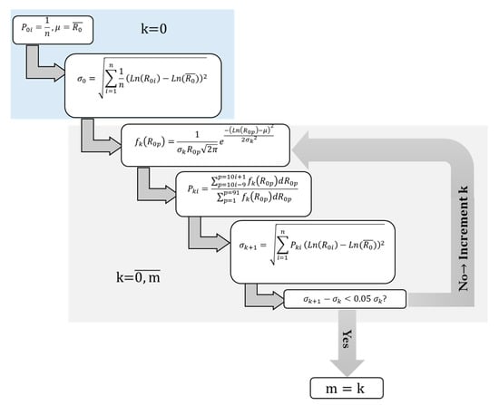
Figure 1.
Schematic illustration of the iterative algorithm used to characterize the equilibrium size distribution within a population of acoustic cavitation bubbles.
The obtained distribution of the number density of bubbles according to their equilibrium radii is considered on a discrete basis by dividing the whole population into n groups with representative ambient radii of 1, 1.5, 2, 2.5, 3, 3.5, 4, 4.5, and 5 µm. The probability of occurrence of each ambient radius in terms of number densities of bubbles is known by the resolution of the iterative algorithm. The number density related to each homogeneous sub-population is retrieved by the application of microscopic and macroscopic energy balances based on Equation (9) [57] and (10) [16,17,44], respectively. Equation (9) represents the energy balance applied on a single acoustic cavitation bubble of a radius evolving in water under an oxygen atmosphere, within which 45 elementary chemical equations [13] are supposed to emerge, giving rise to 9 chemical species, as shown in Table 1.

Table 1.
Adopted scheme of the possible reactions occurring inside an O2/H2O collapsing bubble [13]. M is the third body. A is expressed in (m3/mol∙s) for two body reaction (m6/mol2∙s) for a three-body reaction.
Each elementary reaction in Table 1 is schematized by the general form shown in Equation (10).
In Equation (10), and represent the stoichiometric coefficients in the reactants and products sides, respectively, related to the j-th species. The variation of the molar yield of the j-th species within the i-th homogeneous sub-population due to the chemical mechanism that is then governed by the kinetics equation expressed in Equation (11).
Within the i-th homogeneous sub-population characterized by a common ambient radius (), the number density of bubbles is governed by Equation (12), whose derivation is detailed in our previous research work [16]. Each bubble within the sub-population is characterized by an instantaneous radius , a pressure of gases inside the bubble , and an internal temperature .
In each sub-population, the bubble is supposed to grow starting from the corresponding ambient radius to a maximum size achieved at the end of the expansion phase, and then contracts to a minimum size characterizing the instant of the strong collapse. The instantaneous radius related to the i-th sub-population is governed by the modified Keller-Miksis equation [13,58] shown in Equation (13), which accounts for the non-equilibrium of evaporation and condensation of water molecules at the bubble–liquid interface, as expressed in Equation (14).
In Equation (13), represents the rate of evaporation and condensation of water molecules at the bubble interfaces within the i-th sub-population. is positive in the direction of evaporation, it is given by the Hertz Knudsen law [59], as indicated in Equation (14).
In Equation (14), represents the partial pressure of water vapor inside the bubble volume within the i-th sub-population, while constitutes the accommodation coefficient corresponding to bubbles within the same sub-population. is a function of as indicated by Yasui [13] and Fuster et al. [59].
The system of nonlinear differential Equations (9), (11)–(14) is resolved through the modified Rosenbrock algorithm using MATLAB. The whole algorithm of the characterization of the acoustic cavitation bubbles within the heterogeneous population is schematized in Figure 2. The volume probability within the i-th sub-population and the overall number density of bubbles within the heterogeneous population are calculated following Equations (15) and (16).
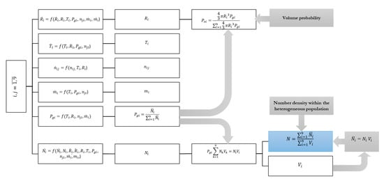
Figure 2.
Schematic illustration of the algorithm applied for characterization of the heterogeneous population of acoustic cavitation bubbles.
is the portion of the liquid volume, hypothetically taken as 1 m3, related to the i-th sub-population, and through which the number of bubbles belonging to this sub-population is calculated by the resolution for of the system of linear equations described in Equation (17).
The rate of the sonochemical production of free radicals within the heterogeneous population is estimated based on the production of a single acoustic cavitation bubble of a given equilibrium radius over 4 acoustic cycles. It is expressed for , and as shown in Equation (18).
These rates are compared to those obtained with the assumption of homogeneous population with equilibrium radii of 1, 1.5, 2, 2.5, 3, 3.5, 4, 4.5, and 5 µm, calculated as shown in Equation (19).
3. Results and Discussion
Before dealing with the statistical approach of the equilibrium size distribution within the heterogeneous population, it is important to inspect the individual response of the representative sub-populations composing the considered sample, ranging from an equilibrium radius of 1 µm to an equilibrium radius of 5 µm, with a conventional step of 0.5 µm. A single acoustic cavitation bubble from each sub-population is dynamically studied under the effect of an acoustic field of 300 kHz and 0.761 W/cm2. The dynamics of oscillation of each acoustic cavitation bubble is simulated over four acoustic cycles, and the results are shown in Figure 3.
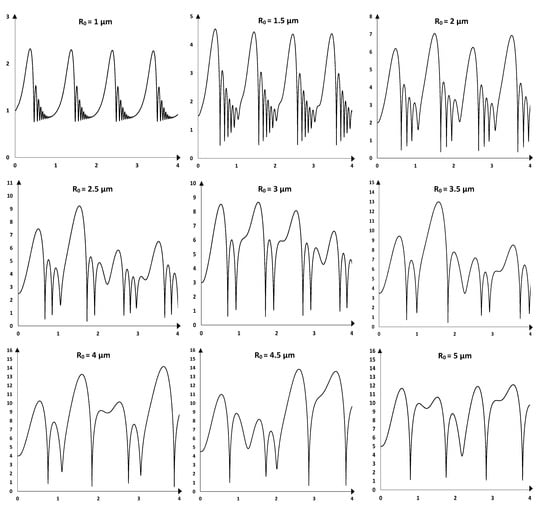
Figure 3.
Simulated bubble radius (vertical axis in µm) over four acoustic cycles (horizontal axis) for acoustic bubbles of ambient radii varying in the range 1–5 µm under an exciting wave of 300 kHz and 1.5 atm. The bubbles are supposed to oscillate in water under oxygen–atmosphere.
From Figure 3, it is observed that the period-1 orbit stability is gradually lost as the ambient radius increases from 1 to 5 µm. The sub-population having a representative ambient radius of 1 µm is composed of stable acoustic cavitation bubbles, the oscillation of the bubble wall is integrally repeated from one acoustic cycle to the other. This is also almost the case with an ambient radius of 1.5 µm. A slight variation is observable starting from 2 µm, as we can notice a difference in the maximum radius attained by the end of the expansion phase during each cycle, with respective values of 6.15, 7.02, 6.17, and 6.86 µm. The oscillation of the bubble wall becomes gradually unstable by moving to sub-populations with a higher equilibrium radius [60]. For instance, with ambient radii comprised between 2.5 and 5 µm, it is remarkable that the variation of the bubble radius as a function of time is completely different from one acoustic cycle to another. It is important to note that the present work considers four acoustic cycles as the simulation time, and this duration may be not enough to characterize the stiffness stability of the oscillator during the steady state period. Thus, the above observations are deemed to apply to the simulated period.
In order to deeply analyze the nature of the bubble dynamics, we suggest reporting the velocity of the bubble wall in function of the dimensionless bubble radius defined as the ratio of the instantaneous radius to the ambient radius. The projection of bubble wall trajectory in the state space [36,61] presented in Figure 4 reveals that starting from an ambient radius of 2.5 µm, the trajectory becomes clearly divergent from the central initial point, demonstrating an unstable behavior. The projection also reveals the extent of variation between the lowest and the highest radius during bubble oscillation, also expressed through the compression ratio. Figure 4 demonstrates that the sub-populations with ambient radii of 2.5 and 3.5 µm know the harshest dynamics of oscillation, with maximum radii of the order of 3.68 and 3.71 folds the ambient radii, and minimum radii of the order of 0.145 and 0.128 folds the ambient radii, respectively. This results in respective compression ratios of 25 and 29. However, owing the unstable oscillation, these ratios are only applicable in both cases to one cycle out of the four, and do not necessarily reflect the severity of the average conditions of temperature and pressure attained during the bubbles’ oscillation within each sub-population.
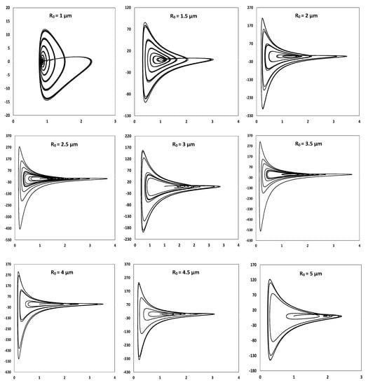
Figure 4.
Bubble wall velocity (vertical axis in m/s) in function of reduced radius (horizontal axis) for acoustic bubbles of ambient radii varying in the range 1–5 µm under an exciting wave of 300 kHz and 1.5 atm.
In terms of composition, most of the sub-populations of the heterogeneous population are characterized by an unstable oscillation. The oscillation would then be chaotic if the observed projections are verified for longer simulation times attaining the steady state. However, the “most” here only refers to 6 sub-populations out of 9, the predominant nature of the bubbles can be deduced only after figuring out the number-based equilibrium size distribution. It is worth noting that with higher acoustic amplitude, most of the sub-population would tend to show unstable oscillation since the zone of stable acoustic cavitation bubbles will become narrow, as shown by Yasui et al. [62].
At present, we suggest examining the probability density of occurrence of each equilibrium size based on the number of bubbles. Considering a log-normal distribution, the iterative algorithm described in the “Computational methodology” section results in the values of standard deviation and probability density reported in Figure 5a,b, respectively.
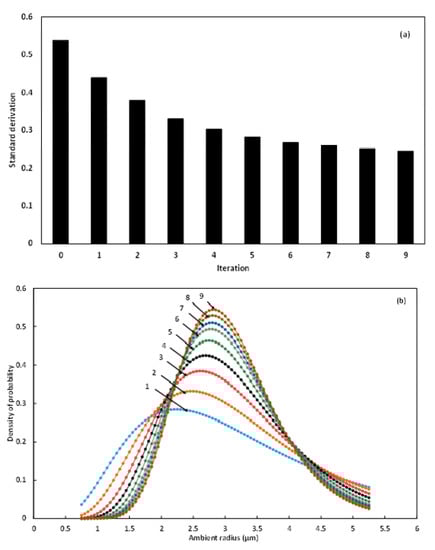
Figure 5.
Standard deviation (a) and probability density (b) of equilibrium radii distribution at successive iteration until convergence.
Figure 5a shows that starting from an initial value of standard deviation of 0.538, the successive iterations converge at the 9th incrementation by achieving less than 5% difference between the 8th and the 9th iterations, with respective values of 0.252 and 0.246. The convergence of the iterative method is linear, the convergence order is 1, and the convergence rate equals 0.4. The conventional convergence condition being attained, the value of the standard deviation is fixed at 0.246. The evolution of the probability density throughout the 9 iterations is reported in Figure 5b. The figure demonstrates that at the first iteration, the highest probability density is observed between 2 and 2.5 µm. With the successive incrementations, the ambient radius corresponding to the highest probability density is gradually shifted to 3 µm.
The 9th curve of log-normal probability density corresponds to the value of standard deviation verifying convergence. It is then considered for the calculation of the number-based equilibrium size distribution, or in other words the probability of occurrence of each sub-population within the heterogeneous cloud expressed in terms of number of bubbles. The probability is retrieved by the integration of the probability density, the retrieved results at each iteration are reported in Figure 6a, and the final considered distribution is presented in Figure 6b.
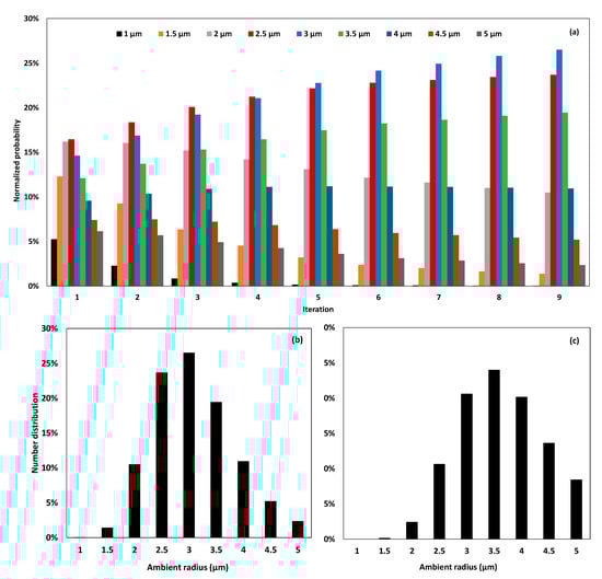
Figure 6.
Normalized probability of equilibrium radii at successive iteration until convergence (a), final number distribution (b), and final volume distribution (c).
Figure 6a demonstrates that starting from a homogeneous probability assumption of 1/9, the log-normal distribution results at the first iteration in close probabilities of sub-populations having ambient radii of 2 and 2.5 µm with a value of 16%, followed by the sub-population of 3 µm with a probability of 14.62%. With the successive incrementation, it is observed that the probability of the sub-population of 1 µm is gradually decreased until becoming almost null at convergence. Simultaneously, the probabilities of the sub-populations of 3 and 3.5 µm are increased at the extent of 2 and 2.5 µm. At convergence, the highest probability is that of the 3 µm sub-population, with a value of 27%, followed by 2.5 µm with a value of 24%, and then 3.5 µm with a value of 19%. This distribution being number based, this means that 27% of the bubbles within the heterogeneous cloud are expected to have an equilibrium radius of 3 µm, while 24% and 19% are expected to have equilibrium radii of 2.5 and 3.5 µm, respectively. In a gas–volume basis, it is interesting to know which portion of void fraction would be attributed to each sub-population, in function of the equilibrium radius, at the equilibrium state. The calculations performed based on Equation (15) return the results reported in Figure 6c. This figure reveals that 24% of the void created by the acoustic cavitation bubbles at equilibrium within the cloud would be attributed to bubbles having an ambient radius of 3.5 µm. Twenty-one percent of this void would result from the bubbles having an ambient radius of 3 µm, while 20% is related to 4 µm bubbles. It is remarkable here that although 4 µm bubbles are not predominant in terms of number, owing to the volume of the single acoustic cavitation bubble at equilibrium, this sub-population represents a major part of the gas volume created by the bubbles at equilibrium within the cloud. It is important to notice that although the size distribution generally refers to number-based probabilities considered at equilibrium, in some cases, it is difficult to figure out whether the distribution is presented based on the number of bubbles or the occupied volume by the gas phase. This specification should be carefully mentioned when dealing with the size distribution of cavitation bubbles, as major differences may result from the volume of the single bubble at a given ambient radius.
In the present section, each sub-population is characterized by a number density of bubbles, calculated using a combination of microscopic and macroscopic energy balances presented in Equations (9) and (10), respectively. The average number density is estimated assuming that each sub-population of index acts as a homogeneous cloud of an ambient radius . The obtained average number densities of bubbles for the 9 sub-populations are presented in Figure 7a. It is observed that the homogeneous sub-population of 1 µm of ambient radius is characterized by the highest number density of 8.8 1012 bubbles∙m−3. This value is followed by 1.3 1012 bubbles∙m−3 related to the homogeneous sub-population of 2 µm. Overall, the retrieved number densities range from 6.9 109 to 8.8 1012 bubbles∙m−3, and the lowest value corresponds to the homogeneous sub-population of 4 µm.
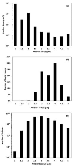
Figure 7.
Number density within homogeneous population (a), distribution of liquid volume (b), and distribution of the number of bubbles (c), in function of the ambient radii.
Based on the previous results, the heterogeneous cloud of acoustic cavitation bubbles evolving within one unit volume of liquid, let us consider it 1 m3, is assumed as a combination of 9 sub-populations of known homogeneous number densities. Each sub-population is then supposed to hypothetically occupy a volume of the liquid, to which the homogeneous number density is applied. The resolution of the system of 9 linear equations described in Equation (17) results in the fractions of liquid volume hypothetically occupied by the 9 sub-populations, presented in Figure 7b. This figure shows that the presence of the sub-population of 4 µm is equivalent to an occupied liquid volume of 29.9%, against 23.3% and 20.3% for 3 and 3.5 µm, respectively. The sub-populations of 1, 1.5, and 2 µm occupy minor fractions that do not exceed 0.15%. According to these fractions, the number of bubbles belonging to each sub-population at equilibrium can be deduced using Equation (17). The results are shown in Figure 7c.
The log-normal distribution of the number of bubbles per equilibrium radius demonstrates that a liquid unit volume of 1 m3 contains a total number of 1.9 1010 bubbles of different equilibrium radii. The 3 µm sub-population being the most probable, as shown in Figure 6b, counts 5.03 109 bubbles. It is directly followed by the sub-population of 2.5 µm, with 4.49 109 bubbles, and then 3.5 µm with 3.69 109 bubbles. The lowest number of bubbles corresponds to the sub-population of 1 µm, with a value of 3.79 106 bubbles.
Compared to the heterogeneous population model, and considering 3 µm as the representative equilibrium radius, it appears that under such assumption, the number density of bubbles would be slightly overestimated, with 2.15 1010 bubbles∙m−3 versus 1.9 1010 bubbles∙m−3 with the heterogeneous population model. The difference is estimated at 11.63%. However, in most of the applications of ultrasound in processes, particularly sonochemistry, the accumulated effects generated within the heterogeneous population are more important than the average number density itself. Thus, we suggest approaching the sonochemical production of free radicals, namely and , under an oxygen atmosphere using both homogeneous model for different ambient radii, and heterogeneous model with the distribution retrieved in Figure 7c. The obtained results are reported in Figure 8.
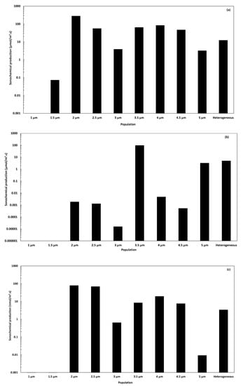
Figure 8.
Sonochemical production rates of (a), (b), and (c) per unit volume of liquid within homogeneous populations of different equilibrium radii and a heterogeneous population.
The rates of the sonochemical production of and have been first estimated at the single bubble scale, considering the 9 different equilibrium radii ranging from 1 to 5 µm, and using Equation (11). The production rates within a homogeneous population of a given ambient radius are calculated using Equation (19), while Equation (18) is used to estimate the rates of production within the heterogeneous population. The results are reported for the three free radicals in Figure 8a–c.
Figure 8a demonstrates that the production of hydroxyl radical attains within the heterogeneous population 12.67 µmol∙m−3∙s−1. This order of magnitude is 4 folds higher than that reported for a homogeneous population of 3 µm of ambient radius. Although this value is representative of the heterogeneous population, the estimation of the sonochemical production of the most significant radical in the oxidation process reveals an important difference between both models of 8.84 µmol∙m−3∙s−1, i.e., 231% higher than the homogeneous model result.
Figure 8b presents the rates of production of hydroperoxyl radical , and the heterogeneous model returns a value of 4.93 µmol∙m−3∙s−1. In this case, the homogeneous model considering the representative ambient radius of 3 µm results in a rate of 0.015 nmol∙m−3∙s−1. The difference between both models reaches a ratio of 3.3 105. The production rate of hydroperoxyl radical within the heterogeneous population is clearly influenced by the production of the 3.5 µm-bubbles, characterized by a homogeneous rate of 96.5 µmol∙m−3∙s−1.
In Figure 8c, the production rate of hydrogen radical attains 3.37 nmol∙m−3∙s−1 according to the heterogeneous model. The homogeneous model considering an ambient radius of 3 µm results in 0.64 nmol∙m−3∙s−1, which is 5.3 folds lower. It appears that the production of hydrogen radical within the heterogeneous population is highly influenced by the 2.5 µm sub-population, showing a rate of 6.89 nmol∙m−3∙s−1.
Among the three free radicals inspected in the present study, it appears that under the considered conditions, the estimation of the sonochemical production rate of hydroperoxyl radical using the homogeneous model at the representative ambient radius is seriously underestimated as compared to the heterogeneous model.
4. Conclusions
A heterogeneous population of acoustic cavitation bubbles with equilibrium radii ranging from 1 to 5 µm has been divided into sub-populations, considering a step of 0.5 µm. The study of the nature of the oscillation dynamics of each sub-population, particularly through the projection of bubble wall trajectory in the state space, revealed that starting from an equilibrium radius of 2.5 µm, the oscillation becomes unstable, tending to chaotic.
The distribution of the number of bubbles as a function of the equilibrium radii has been studied based on a statistical algorithm using the log-normal law. The algorithm converged after 9 iterations, revealing that 3 µm is the most predominant population in number of bubbles, with a probability of 27%. The expression of the distribution based on the gas phase volume demonstrated that the highest probability is attained by the sub-population of 4 µm, with a value of 24%.
The number density of bubbles within the heterogeneous population has been estimated through the calculation of the homogeneous number densities and the volume fractions of the liquid related to each sub-population. A value of 1.9 × 10¹⁰ bubbles∙m−3 has been retrieved using the heterogeneous approach, which is 11.63% higher than the value given by the homogeneous model considering 3 µm as a representative ambient radius. Considering only the representative ambient radius (the most probable) can result in an acceptable order of magnitude of average number density of bubbles within the heterogeneous population, the study of the accumulated effects resulting from all the sub-populations composing the heterogeneous cloud is important when it comes to the sonochemical production of the heterogeneous population.
The simulation of the sonochemical production of free radicals under oxygen atmosphere using the homogeneous and the heterogeneous approach demonstrated that a difference ranging from 5 to 3.3 × 10⁵ folds could be noticed when comparing the productions of and using both models.
Author Contributions
K.K.: conceptualization, methodology, software, validation, formal analysis, investigation, writing—original draft preparation, and writing—review and editing; O.H.: supervision, conceptualization, methodology, project administration, resources, funding acquisition, investigation, validation, and writing—review and editing; A.A.: visualization, validation, and writing—review and editing. All authors have read and agreed to the published version of the manuscript.
Funding
This work was financially supported the Deanship of Scientific Research at King Saud University through research group No. RG-1441-501.
Institutional Review Board Statement
Not applicable.
Informed Consent Statement
Not applicable.
Data Availability Statement
Not applicable.
Acknowledgments
The authors extend their appreciation to the Deanship of Scientific Research at King Saud University for the funding of this work through research group No. RG-1441-501.
Conflicts of Interest
The authors declare no conflict of interest.
References
- Yasui, K. Acoustic Cavitation and Bubble Dynamics; Pollet, B.G., Ashokkumar, M., Eds.; Springer Briefs in Molecular Science: Ultrasound and Sonochemistry: Nagoya, Japan, 2017. [Google Scholar]
- Kentish, S.; Ashokkumar, M. The Physical and Chemical Effects of Ultrasound. In Ultrasound Technologies for Food and Bioprocessing; Elsevier: New York, NY, USA, 2010; pp. 1–19. [Google Scholar]
- Grieser, F.; Choi, P.-K.; Enomoto, N.; Harada, H.; Okitsu, K.; Yasui, K. Sonochemistry and the Acoustic Bubble; Elsevier: Amesterdam, The Netherlands, 2015. [Google Scholar]
- Gong, C.; Hart, D.P. Ultrasound induced cavitation and sonochemical yields. J. Acoust. Soc. Am. 1998, 104, 2675–2682. [Google Scholar] [CrossRef]
- Thompson, L.H.; Doraiswamy, L.K. Sonochemistry: Science and Engineering. Ind. Eng. Chem. Res. 1999, 38, 1215–1249. [Google Scholar] [CrossRef]
- Lim, M.; Son, Y.; Khim, J. Frequency effects on the sonochemical degradation of chlorinated compounds. Ultrason. Sonochemistry 2011, 18, 460–465. [Google Scholar] [CrossRef]
- Merouani, S.; Hamdaoui, O.; Saoudi, F.; Chiha, M.; Pétrier, C. Influence of bicarbonate and carbonate ions on sonochemical degradation of Rhodamine B in aqueous phase. J. Hazard. Mater. 2010, 175, 593–599. [Google Scholar] [CrossRef] [PubMed]
- Navarro, N.M.; Chave, T.; Pochon, P.; Bisel, I.; Nikitenko, S.I. Effect of Ultrasonic Frequency on the Mechanism of Formic Acid Sonolysis. J. Phys. Chem. B 2011, 115, 2024–2029. [Google Scholar] [CrossRef] [PubMed]
- Anto, T.; Bauchat, P.; Foucaud, A.; Fujita, M.; Kimura, T.; Sohmiya, H. Sonochemical switching from ionic to radical pathways in the reactions of styrene and trans-β-Methylstyrene with lead tetraacetate. Tetrahedron Lett. 1991, 32, 6379–6382. [Google Scholar] [CrossRef]
- Kerboua, K.; Hamdaoui, O.; Islam, M.H.; Alghyamah, A.; Hansen, H.E.; Pollet, B.G. Low carbon ultrasonic production of alternate fuel: Operational and mechanistic concerns of the sonochemical process of hydrogen generation under various scenarios. Int. J. Hydrogen Energy 2021, 46, 26770–26787. [Google Scholar] [CrossRef]
- Kerboua, K.; Hamdaoui, O.; Alghyamah, A. Energy balance of high-energy stable acoustic cavitation within dual-frequency sonochemical reactor. Ultrason. Sonochemistry 2021, 73, 105471. [Google Scholar] [CrossRef]
- Merouani, S.; Hamdaoui, O.; Rezgui, Y.; Guemini, M. Computational engineering study of hydrogen production via ultrasonic cavitation in water. Int J. Hydrogen Energy 2016, 41, 832–844. [Google Scholar] [CrossRef]
- Yasui, K. Alternative model of single-bubble sonoluminescence. Phys. Rev. E 1997, 56, 6750–6760. [Google Scholar] [CrossRef]
- Sivasankar, T.; Moholkar, V.S. Physical insights into the sonochemical degradation of recalcitrant organic pollutants with cavitation bubble dynamics. Ultrason. Sonochemistry 2009, 16, 769–781. [Google Scholar] [CrossRef]
- Merouani, S.; Ferkous, H.; Hamdaoui, O.; Rezgui, Y.; Guemini, M. A method for predicting the number of active bubbles in sonochemical reactors. Ultrason. Sonochemistry 2015, 22, 51–58. [Google Scholar] [CrossRef]
- Kerboua, K.; Hamdaoui, O. Void fraction, number density of acoustic cavitation bubbles, and acoustic frequency: A numerical investigation. J. Acoust. Soc. Am. 2019, 146, 2240–2252. [Google Scholar] [CrossRef] [PubMed]
- Kerboua, K.; Hamdaoui, O.; Alghyamah, A. Predicting the Sonochemical Efficiency for Water Decontamination: An Upscaled Numerical Approach. Chem. Eng. Technol. 2020, 44, 273–282. [Google Scholar] [CrossRef]
- Hao, Y.; Oguz, H.N.; Prosperetti, A. The action of pressure-radiation forces on pulsating vapor bubbles. Phys. Fluids 2001, 13, 1167–1177. [Google Scholar] [CrossRef][Green Version]
- Mettin, R.; Akhatov, I.; Parlitz, U.; Ohl, C.D.; Lauterborn, W. Bjerknes forces between small cavitation bubbles in a strong acoustic field. Phys. Rev. E 1997, 56, 2924–2931. [Google Scholar] [CrossRef]
- Zhang, Y.; Li, S. The secondary Bjerknes force between two gas bubbles under dual-frequency acoustic excitation. Ultrason. Sonochemistry 2016, 29, 129–145. [Google Scholar] [CrossRef]
- Iida, Y.; Ashokkumar, M.; Tuziuti, T.; Kozuka, T.; Yasui, K.; Towata, A.; Lee, J. Bubble population phenomena in sonochemical reactor: II. Estimation of bubble size distribution and its number density by simple coalescence model calculation. Ultrason. Sonochemistry 2010, 17, 480–486. [Google Scholar] [CrossRef] [PubMed]
- Yasui, K. Influence of ultrasonic frequency on multibubble sonoluminescence. J. Acoust. Soc. Am. 2002, 112, 1405–1413. [Google Scholar] [CrossRef] [PubMed]
- Colonius, T.; Hagmeijer, R.; Ando, K.; Brennen, C.E. Statistical equilibrium of bubble oscillations in dilute bubbly flows. Phys. Fluids 2008, 20, 040902. [Google Scholar] [CrossRef]
- Ida, M. Multibubble cavitation inception. Phys. Fluids 2009, 21, 113302. [Google Scholar] [CrossRef]
- Yasui, K.; Iida, Y.; Tuziuti, T.; Kozuka, T.; Towata, A. Strongly interacting bubbles under an ultrasonic horn. Phys. Rev. E 2008, 77, 016609. [Google Scholar] [CrossRef]
- Shen, Y.; Zhang, L.; Wu, Y.; Chen, W. The role of the bubble–bubble interaction on radial pulsations of bubbles. Ultrason. Sonochemistry 2021, 73, 105535. [Google Scholar] [CrossRef]
- D’Hondt, L.; Cavaro, M.; Payan, C.; Mensah, S. Acoustical characterisation and monitoring of microbubble clouds. Ultrasonics 2019, 96, 10–17. [Google Scholar] [CrossRef] [PubMed]
- Desai, P.D.; Ng, W.C.; Hines, M.J.; Riaz, Y.; Tesar, V.; Zimmerman, W.B. Comparison of Bubble Size Distributions Inferred from Acoustic, Optical Visualisation, and Laser Diffraction. Colloids Interfaces 2019, 3, 65. [Google Scholar] [CrossRef]
- Brotchie, A.; Grieser, F.; Ashokkumar, M. Effect of Power and Frequency on Bubble-Size Distributions in Acoustic Cavitation. Phys. Rev. Lett. 2009, 102, 084302. [Google Scholar] [CrossRef] [PubMed]
- Avvaru, B.; Pandit, A.B. Oscillating bubble concentration and its size distribution using acoustic emission spectra. Ultrason. Sonochemistry 2009, 16, 105–115. [Google Scholar] [CrossRef] [PubMed]
- Xu, S.; Zong, Y.; Li, W.; Zhang, S.; Wan, M. Bubble size distribution in acoustic droplet vaporization via dissolution using an ultrasound wide-beam method. Ultrason. Sonochemistry 2014, 21, 975–983. [Google Scholar] [CrossRef] [PubMed]
- Reuter, F.; Lesnik, S.; Ayaz-Bustami, K.; Brenner, G.; Mettin, R. Bubble size measurements in different acoustic cavitation structures: Filaments, clusters, and the acoustically cavitated jet. Ultrason. Sonochemistry 2019, 55, 383–394. [Google Scholar] [CrossRef]
- Calvisi, M.L.; Lindau, O.; Blake, J.R.; Szeri, A.J. Shape stability and violent collapse of microbubbles in acoustic traveling waves. Phys. Fluids 2007, 19, 47101. [Google Scholar] [CrossRef]
- Akhatov, I.S.; Konovalova, S.I. Regular and chaotic dynamics of a spherical bubble. J. Appl. Math. Mech. 2005, 69, 575–584. [Google Scholar] [CrossRef]
- Zhang, Y.; Gao, Y.; Du, X. Stability mechanisms of oscillating vapor bubbles in acoustic fields. Ultrason. Sonochemistry 2018, 40, 808–814. [Google Scholar] [CrossRef] [PubMed]
- Zhang, Y. Chaotic oscillations of gas bubbles under dual-frequency acoustic excitation. Ultrason. Sonochemistry 2018, 40, 151–157. [Google Scholar] [CrossRef]
- Hegedűs, F.; Lauterborn, W.; Parlitz, U.; Mettin, R. Non-feedback technique to directly control multistability in nonlinear oscillators by dual-frequency driving: GPU accelerated topological analysis of a bubble in water. Nonlinear Dyn. 2018, 94, 273–293. [Google Scholar] [CrossRef]
- Klapcsik, K.; Hegedűs, F. Study of non-spherical bubble oscillations under acoustic irradiation in viscous liquid. Ultrason. Sonochemistry 2019, 54, 256–273. [Google Scholar] [CrossRef]
- Klapcsik, K.; Hegedűs, F. The effect of high viscosity on the evolution of the bifurcation set of a periodically excited gas bubble. Chaos Solitons Fractals 2017, 104, 198–208. [Google Scholar] [CrossRef][Green Version]
- Kerboua, K.; Hamdaoui, O. Numerical investigation of the effect of dual frequency sonication on stable bubble dynamics. Ultrason. Sonochemistry 2018, 49, 325–332. [Google Scholar] [CrossRef]
- Kerboua, K.; Hamdaoui, O. Oxidants Emergence under Dual-Frequency Sonication within Single Acoustic Bubble: Effects of Frequency Combinations. Iran. J. Chem. Chem. Eng. 2021, 40, 323–332. [Google Scholar] [CrossRef]
- Burdin, F.; Tsochatzidis, N.; Guiraud, P.; Wilhelm, A.; Delmas, H. Characterisation of the acoustic cavitation cloud by two laser techniques. Ultrason. Sonochemistry 1999, 6, 43–51. [Google Scholar] [CrossRef]
- Duraiswami, R.; Prabhukumar, S.; Chahine, G.L. Bubble counting using an inverse acoustic scattering method. J. Acoust. Soc. Am. 1998, 104, 2699–2717. [Google Scholar] [CrossRef]
- Kerboua, K.; Hamdaoui, O.; Alghyamah, A. Acoustic frequency and optimum sonochemical production at single and multi-bubble scales: A modeling answer to the scaling dilemma. Ultrason. Sonochemistry 2021, 70, 105341. [Google Scholar] [CrossRef]
- Wayment, D.G.; Casadonte, D.J. Frequency effect on the sonochemical remediation of alachlor. Ultrason. Sonochemistry 2002, 9, 251–257. [Google Scholar] [CrossRef]
- Koda, S.; Kimura, T.; Kondo, T.; Mitome, H. A standard method to calibrate sonochemical efficiency of an individual reaction system. Ultrason. Sonochemistry 2003, 10, 149–156. [Google Scholar] [CrossRef]
- Mark, G.; Tauber, A.; Laupert, R.; Schuchmann, H.-P.; Schulz, D.; Mues, A.; von Sonntag, C. OH-radical formation by ultrasound in aqueous solution–Part II: Terephthalate and Fricke dosimetry and the influence of various conditions on the sonolytic yield. Ultrason. Sonochemistry 1998, 5, 41–52. [Google Scholar] [CrossRef]
- Chiha, M.; Hamdaoui, O.; Baup, S.; Gondrexon, N. Sonolytic degradation of endocrine disrupting chemical 4-cumylphenol in water. Ultrason. Sonochemistry 2011, 18, 943–950. [Google Scholar] [CrossRef]
- Didenko, Y.T.; Suslick, K.S. The energy efficiency of formation of photons, radicals and ions during single-bubble cavitation. Nature 2002, 418, 394–397. [Google Scholar] [CrossRef] [PubMed]
- Kim, K.Y.; Byun, K.-T.; Kwak, H.-Y. Temperature and pressure fields due to collapsing bubble under ultrasound. Chem. Eng. J. 2007, 132, 125–135. [Google Scholar] [CrossRef]
- Merouani, S.; Hamdaoui, O.; Haddad, B. Acoustic cavitation in 1-butyl-3-methylimidazolium bis(triflluoromethyl-sulfonyl)imide based ionic liquid. Ultrason. Sonochemistry 2018, 41, 143–155. [Google Scholar] [CrossRef]
- Kulkarni, A.A.; Joshi, J.B. Bubble formation and bubble rise velocity in gas-liquid systems. Ind. Eng. Chem. Res. 2005, 44, 5873–5931. [Google Scholar] [CrossRef]
- Pandit, A.B.; Varley, J.; Thorpe, R.B.; Davidson, J. Measurement of bubble size distribution: An acoustic technique. Chem. Eng. Sci. 1992, 47, 1079–1089. [Google Scholar] [CrossRef]
- Xu, W.; Tzanakis, I.; Srirangam, P.; Terzi, S.; Mirihanage, W.U.; Eskin, D.G.; Mathiesen, R.H.; Horsfield, A.P.; Lee, P.D. In Situ Synchrotron Radiography of Ultrasound Cavitation in a Molten Al-10Cu Alloy. In Proceedings of the TMS 2015 Annual Meeting Supplemental Proceedings TMS (The Minerals, Metals & Materials Society), Orlando, FL, USA, 15–19 March 2015; pp. 61–66. [Google Scholar]
- Merouani, S.; Hamdaoui, O.; Rezgui, Y.; Guemini, M. Effects of ultrasound frequency and acoustic amplitude on the size of sonochemically active bubbles-Theoretical study. Ultrason Sonochemistry 2013, 20, 815–819. [Google Scholar] [CrossRef] [PubMed]
- Caruthers, J.W. Lognormal bubble size distributions. J. Acoust. Soc. Am. 2017, 142, 2534. [Google Scholar] [CrossRef]
- Kerboua, K.; Hamdaoui, O. Ultrasonic waveform upshot on mass variation within single cavitation bubble: Investigation of physical and chemical transformations. Ultrason. Sonochemistry 2018, 42, 508–516. [Google Scholar] [CrossRef] [PubMed]
- Yasui, K. Variation of Liquid Temperature at Bubble Wall near the Sonoluminescence Threshold. J. Phys. Soc. Jpn. 1996, 65, 2830–2840. [Google Scholar] [CrossRef]
- Fuster, D.; Hauke, G.; Dopazo, C. Influence of the accommodation coefficient on nonlinear bubble oscillations. J. Acoust. Soc. Am. 2010, 128, 5–10. [Google Scholar] [CrossRef]
- Kerboua, K.; Hamdaoui, O. Sonochemistry in Green Processes: Modeling, Experiments, and Technology. In Sustainable Green Chemical Processes and Their Allied Applications; Springer: Cham, Switzerland, 2020; p. 603. [Google Scholar]
- Kerboua, K.; Hamdaoui, O. Sonochemical production of hydrogen: Enhancement by summed harmonics excitation. Chem. Phys. 2019, 519, 27–37. [Google Scholar] [CrossRef]
- Yasui, K.; Tuziuti, T.; Lee, J.; Kozuka, T.; Towata, A.; Iida, Y. The range of ambient radius for an active bubble in sonoluminescence and sonochemical reactions. J. Chem. Phys. 2008, 128, 184705. [Google Scholar] [CrossRef] [PubMed]


Publisher’s Note: MDPI stays neutral with regard to jurisdictional claims in published maps and institutional affiliations. |
© 2021 by the authors. Licensee MDPI, Basel, Switzerland. This article is an open access article distributed under the terms and conditions of the Creative Commons Attribution (CC BY) license (https://creativecommons.org/licenses/by/4.0/).