
Experimental Verification of CFD Simulation When Evaluating the Operative Temperature and Mean Radiation Temperature for Radiator Heating and Floor Heating


Abstract
1. Introduction
Operative Temperature
2. Trends in Indoor Environment Simulation for Heating Systems
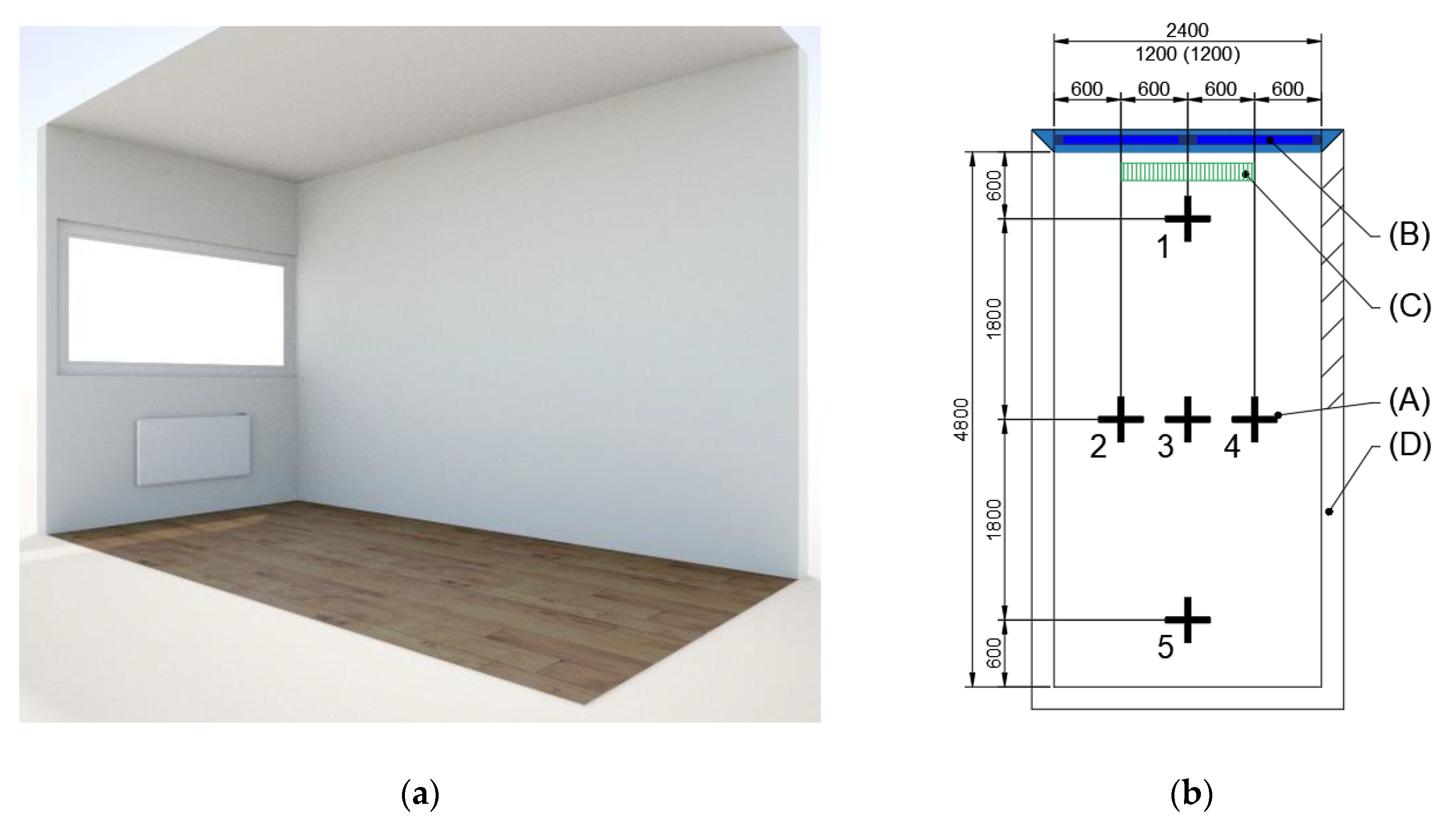
3. Experimental Verification of CFD Simulation
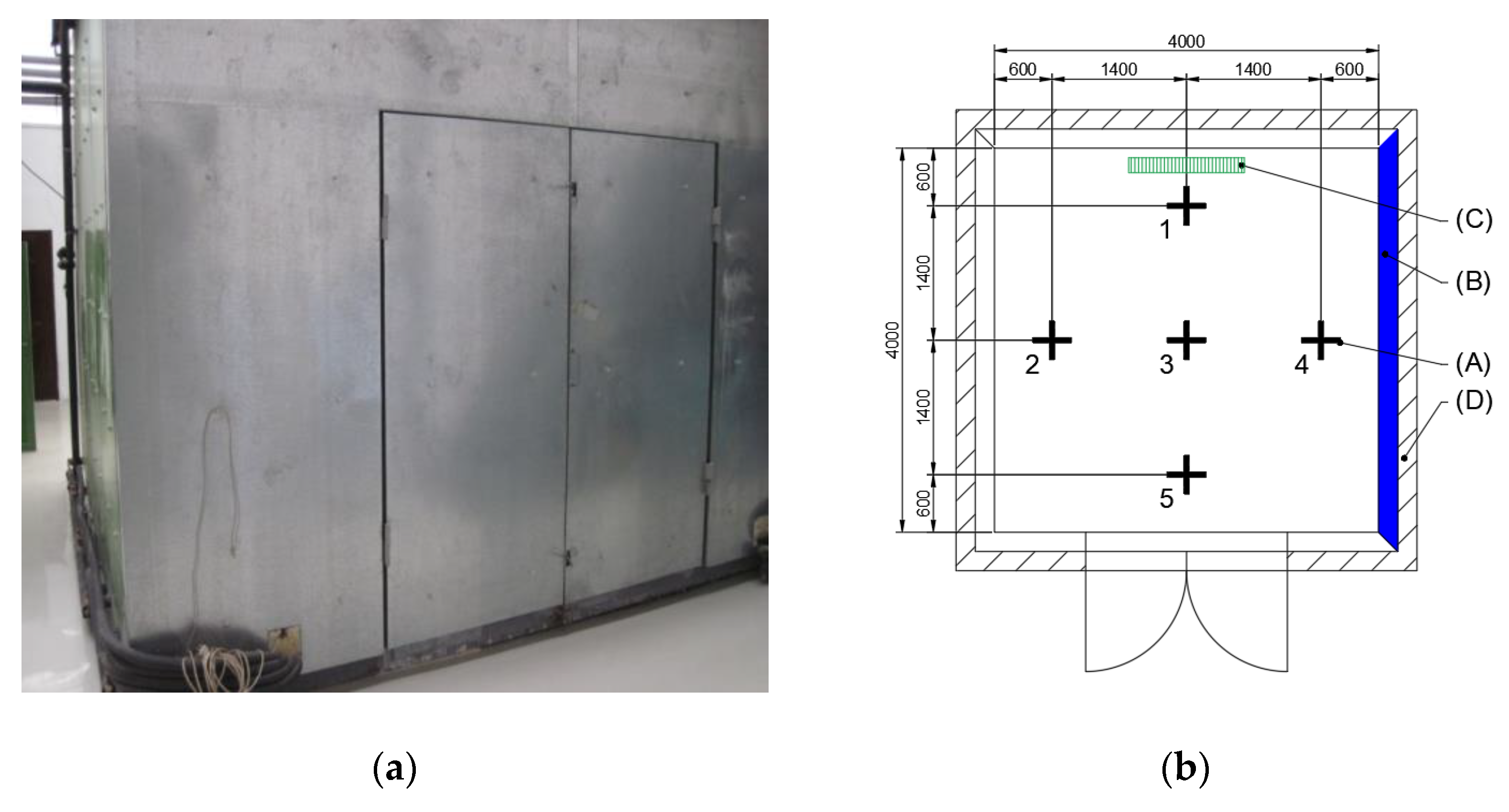
3.1. Thermostatic Chamber
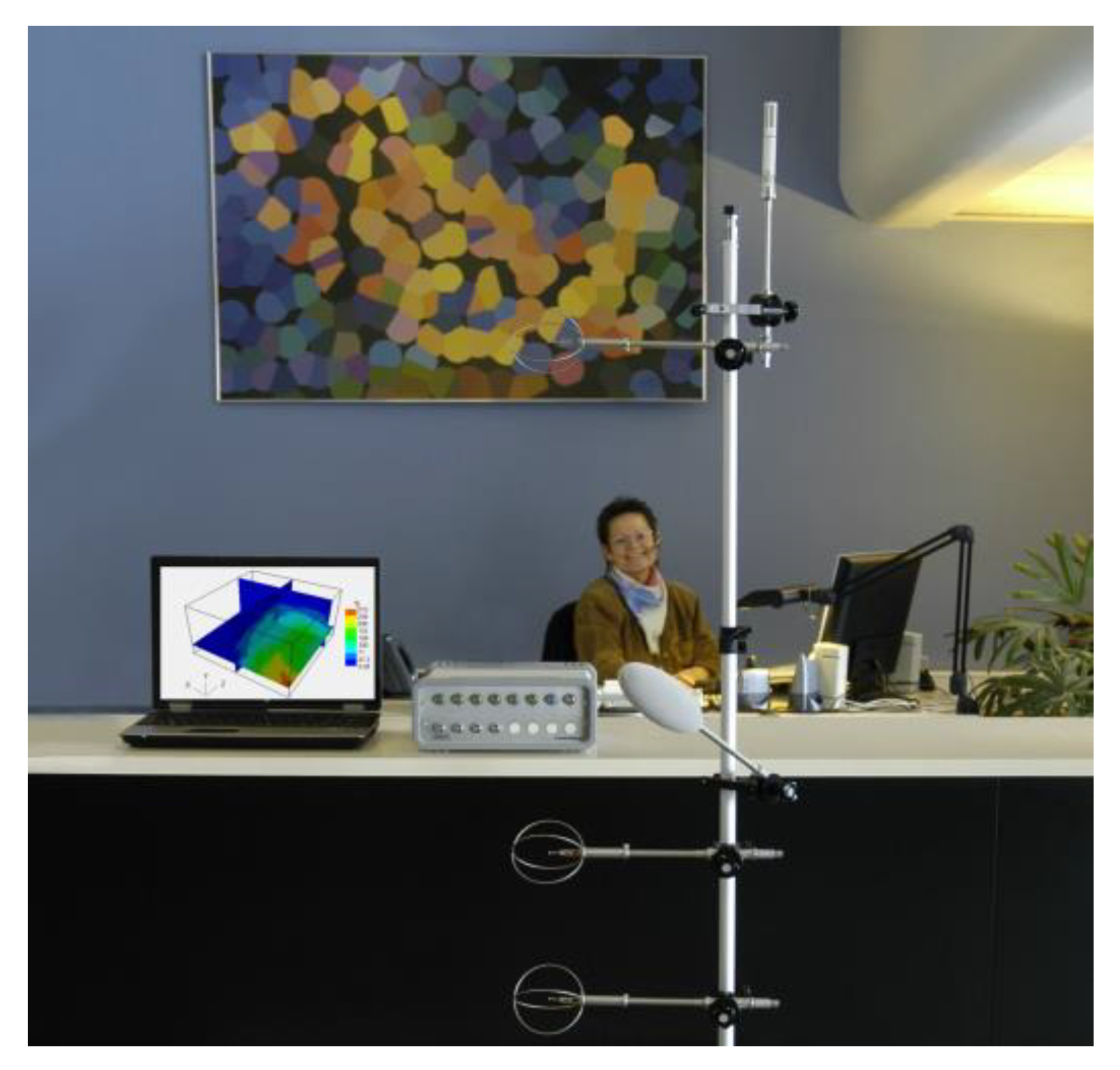
3.2. Measuring Device
3.3. Methodology
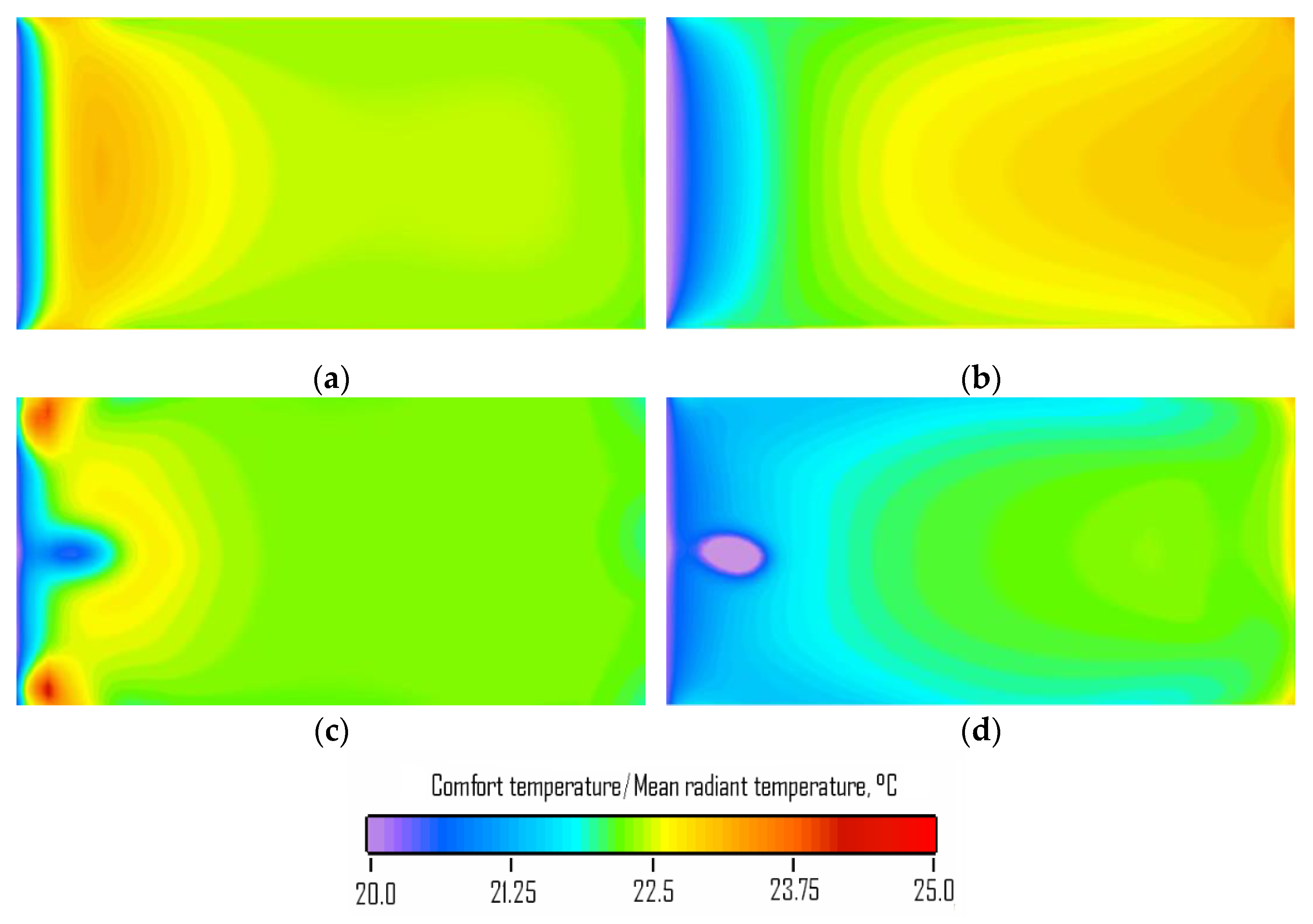
3.4. Results
4. Discussion
5. Conclusions
Author Contributions
Funding
Institutional Review Board Statement
Informed Consent Statement
Data Availability Statement
Conflicts of Interest
References
- Fanger, P.O. Thermal Comfort: Analysis and Applications in Environmental Engineering; McGraw-Hill: New York, NY, USA, 1972. [Google Scholar]
- Kabele, K.; Kabrhel, M. Low-energy building heating system modelling. In Proceedings of the Eighth International IBPSA Conference, Eindhoven, The Netherlands, 11–14 August 2003. [Google Scholar]
- Tzbinfo. Available online: https://vytapeni.tzb-info.cz/teorie-a-schemata/1422-modelovani-operativni-teploty (accessed on 10 March 2021).
- Olesen, B.W.; Mortensen, E.; Thorshauge, J. Thermal Comfort in a Room Heated by Different Methods; Technical Paper no. 2256 Los Angeles Meeting; ASHRAE Transactions: Los Angeles, CA, USA, 1980; Volume 86. [Google Scholar]
- Hutter, E. Comparison of different heat emitters in respect of thermal comfort and energy consumption. In Proceedings of the International Centre for Heat and Mass Transfer, Heat and Mass Transfer in Building Materials and Structures, Dubrovnik, Yugoslavia, 20–24 May 1991; pp. 753–769. [Google Scholar]
- Eijdems, H.H.E.W.; Boerstra, A.C. Low Temperature Heating Systems: Impact on IAQ, Thermal Comfort and Energy Consumption. 2000, pp. 1–6. Available online: https://www.aivc.org/sites/default/files/members_area/medias/pdf/Conf/1999/paper002.pdf (accessed on 3 December 2019).
- Juusela, M.A. Heating and Cooling with Focus on Increased Energy Efficiency and Improved Comfort: Guidebook to IEAAAA ECBCS Annex 37 Low Exergy Systems for Heating and Cooling of Buildings; Summary Report; VTT Technical Research Centre of Finland: Espoo, Finland, 2000. [Google Scholar]
- Gagge, A.P. The linearity criterion as applied to partitional calorimetry. Am. J. Physiol. 1946, 116, 656–668. [Google Scholar] [CrossRef]
- Houghten, F.C.; Yagloglou, C.P. Determining lines of equal comfort. Trans. Am. Soc. Heat. Vent. Eng. 1923, 29, 165–176. [Google Scholar]
- Gagge, A.P.; Fobelets, L.G.; Berglund, L.G. A standard predictive index of human response to the thermal environment. ASHARE Trans. 1986, 92, 709–731. [Google Scholar]
- Krawczyk, B. The Heat Balance of the Human Body as Basis for the Bioclimatic Divide of the Health Resort Iwonicz; Przylibski, A., Jurek, W.A., Eds.; POLSKA AKADEMIA NAUK: Wroclaw Poland, 1979. [Google Scholar]
- Kitawaga, K.; Komodo, N.; Hayano, H.; Tanabe, S. Effect of humidity and small air movement on thermal comfort under a radiant cooling ceiling by subjective experiments. Energy Build. 1999, 30, 185–193. [Google Scholar] [CrossRef]
- Simmonds, P. Practical applications of radiant heating and cooling to maintain comfort conditions. ASHRAE Trans. 1996, 102, 659–666. [Google Scholar]
- Wikipedia. Available online: https://en.wikipedia.org/wiki/Operative_temperature (accessed on 10 March 2021).
- Nilsson, H.O. Comfort Climate Evaluation with Thermal Manikin Methods and Computer Simulation Models, 3rd ed.; National Institute for Working Life: Stockholm, Sweden, 2004; p. 37. [Google Scholar]
- Thermal Environmental Conditions for Human Occupancy; ANSI/ASHRAE Standard 55-2010; American Society of Heating, Refrigeratingand Air-Conditioning Engineers, Inc.: Atlanta, GA, USA, 2011; pp. 1–44.
- Kuznik, F.; Rusaouën, G.; Brau, J. Experimental and numerical study of a full scale ventilated enclosure: Comparison of four two equations closure turbulence models. Build. Environ. 2007, 42, 1043–1053. [Google Scholar] [CrossRef]
- Myhren, J.A.; Holmberg, S. Flow patterns and thermal comfort in a room with panel, floor and wall heating. Energy Build. 2008, 40, 524–536. [Google Scholar] [CrossRef]
- Rohdin, P.; Moshfegh, B. Numerical predictions of indoor climate in large industrial premises. A comparison between different k–e models supported by field measurements. Build. Environ. 2007, 42, 3872–3882. [Google Scholar] [CrossRef]
- Stamou, A.I.; Katsiris, I.; Schaelin, A. Evaluation of thermal comfort in Galatsi Arena of the Olympics “Athens 2004” using a CFD model. Appl. Therm. Eng. 2008, 28, 1206–1215. [Google Scholar] [CrossRef]
- Nilsson, H.O. Thermal comfort evaluation with virtual manikin methods. Build. Environ. 2007, 42, 4000–4005. [Google Scholar] [CrossRef]
- Miyanaga, T.; Urabe, W.; Nakano, Y. Simplified human body model for evaluating thermal radiant environment in a radiant cooled space. Build. Environ. 2001, 36, 801–808. [Google Scholar] [CrossRef]
- Myhren, J.A.; Holmberg, S. Comfort temperatures and operative temperatures in an office with different heating methods. In Proceedings of the Healthy Buildings Conference, Lisbon, Portugal, 4–8 June 2006. [Google Scholar]
- DANTEC DYNAMICS. Available online: https://www.dantecdynamics.com/comfortsense (accessed on 3 December 2019).
- Petras, D. Vykurovanie Rodinných a Bytových Domov; Jaga Group: Bratislava, Slovakia, 2005; pp. 13–25. [Google Scholar]
- Abe, K.; Kondoh, T.; Nagano, Y. A new turbulence model for predicting fluid flow and heat transfer in separating and reattaching flows—I. Flow field calculations. Int. J. Heat Mass Transf. 1994, 37, 139–151. [Google Scholar] [CrossRef]
- Buratti, C.; Palladino, D.; Moretti, E. Prediction of Indoor Conditions And Thermal Comfort Using CFD Simulations: A Case Study Based On Experimental Data. Energy Procedia 2017, 126, 115–122. [Google Scholar] [CrossRef]
- Liu, J.; Heidarinejad, M.; Nikkho, S.K.; Mattise, N.W.; Srebric, J. Quantifying Impacts of Urban Microclimate on a Building Energy Consumption—A Case Study. Sustainability 2019, 11, 4921. [Google Scholar] [CrossRef]
- Hormigos-Jimenez, S.; Padilla-Marcos, M.Á.; Meiss, A.; Gonzalez-Lezcano, R.A.; Feijó-Muñoz, J. Computational fluid dynamics evaluation of the furniture arrangement for ventilation efficiency. Build. Serv. Eng. Res. Technol. 2018, 39, 557–571. [Google Scholar] [CrossRef]
- Soleimani-Mohseni, M.; Thomas, B.; Fahlén, P. Estimation of operative temperature in buildings using artificial neural networks. Energy Build. 2006, 38, 635–640. [Google Scholar] [CrossRef]
- Corgnati, S.P.; Fabrizio, E.; Filippi, M. The impact of indoor thermal conditions, system controls and building types on the building energy demand. Energy Build. 2008, 40, 627–636. [Google Scholar] [CrossRef]
- Kalmár, F.; Kalmár, T. Interrelation between mean radiant temperature and room geometry. Energy Build. 2012, 55, 414–421. [Google Scholar] [CrossRef]
- Hashimoto, Y. Numerical study on airflow in an office room with a displacement ventilation system. In Proceedings of the Building Simulation, Montréal, QC, Canada, 15–18 August 2005; pp. 381–387. [Google Scholar]
- Kajiya, R.; Hiruta, K.; Sakai, K.; Ono, H.; Toshihiko, S. Thermal environment prediction using CFD with a virtual mannequin model and experiment with subject in a floor heating room. In Proceedings of the Building Simulation 2011, Sydney, Australia, 14–16 November 2011. [Google Scholar]
- Chung, J.D.; Hong, H.; Yoo, H. Analysis on the impact of mean radiant temperature for the thermal comfort of underfloor air distribution systems. Energy Build. 2010, 42, 2353–2359. [Google Scholar] [CrossRef]
- Chen, Q.; Srebic, J. How to Verify, Validate, and Report Indoor Environment Modelling CFD Analyses. HVAC&R Res. 2001, 8, 201–216. [Google Scholar]
- Chen, Q.; Srebic, J. A procedure for verification, validation, and reporting of indoor environment CFD analyses. HVAC R Res. 2002, 8, 201–216. [Google Scholar] [CrossRef]


| Measured Parameters | Range to Guarantee the Stated Measurement Inaccuracy | Guaranteed Measurement Inaccuracy |
|---|---|---|
| ta—air temperature | 0–45 °C | ±0.2 °C |
| v—air flow velocity | 0–1 m·s−1 | ±0.02 m·s−1 or ±2% |
| to—operative temperature | 10–40 °C | ±0.2 °C |
| Heating System | Measurement Position | Simulation [23] | Experiment | Δtmr (°C) | Δto (°C) | ||
|---|---|---|---|---|---|---|---|
| tmr (°C) | to (°C) | tmr (°C) | to (°C) | ||||
| Radiator | 1 | 23.2 | 22.8 | 20.7 | 21.3 | 2.5 | 1.5 |
| 2 | 22.2 | 22.0 | 20.5 | 21.1 | 1.7 | 0.9 | |
| 3 | 22.0 | 22.0 | 20.5 | 21.1 | 1.5 | 0.9 | |
| 4 | 22.2 | 22.0 | 20.5 | 21.1 | 1.7 | 0.9 | |
| 5 | 22.0 | 22.0 | 20.8 | 21.3 | 1.2 | 0.7 | |
| Floor heating | 1 | 21.6 | 20.5 | 21.3 | 21.7 | 0.3 | −1.2 |
| 2 | 22.5 | 22.0 | 21.7 | 21.9 | 0.8 | 0.1 | |
| 3 | 22.8 | 22.0 | 21.6 | 22.0 | 1.2 | 0.0 | |
| 4 | 22.5 | 22.0 | 21.1 | 21.5 | 1.4 | 0.5 | |
| 5 | 23.2 | 22.5 | 21.7 | 22.1 | 1.5 | 0.4 | |
Publisher’s Note: MDPI stays neutral with regard to jurisdictional claims in published maps and institutional affiliations. |
© 2021 by the authors. Licensee MDPI, Basel, Switzerland. This article is an open access article distributed under the terms and conditions of the Creative Commons Attribution (CC BY) license (https://creativecommons.org/licenses/by/4.0/).
Share and Cite
Mičko, P.; Kapjor, A.; Holubčík, M.; Hečko, D. Experimental Verification of CFD Simulation When Evaluating the Operative Temperature and Mean Radiation Temperature for Radiator Heating and Floor Heating. Processes 2021, 9, 1041. https://doi.org/10.3390/pr9061041
Mičko P, Kapjor A, Holubčík M, Hečko D. Experimental Verification of CFD Simulation When Evaluating the Operative Temperature and Mean Radiation Temperature for Radiator Heating and Floor Heating. Processes. 2021; 9(6):1041. https://doi.org/10.3390/pr9061041
Chicago/Turabian StyleMičko, Pavol, Andrej Kapjor, Michal Holubčík, and Dávid Hečko. 2021. "Experimental Verification of CFD Simulation When Evaluating the Operative Temperature and Mean Radiation Temperature for Radiator Heating and Floor Heating" Processes 9, no. 6: 1041. https://doi.org/10.3390/pr9061041
APA StyleMičko, P., Kapjor, A., Holubčík, M., & Hečko, D. (2021). Experimental Verification of CFD Simulation When Evaluating the Operative Temperature and Mean Radiation Temperature for Radiator Heating and Floor Heating. Processes, 9(6), 1041. https://doi.org/10.3390/pr9061041