A Similarity Model of the Cooling Process of Fluids during Transportation ^†

Abstract

This article presents a description of a novel method for the identification of a decrease in the temperature of a liquid medium transported by railroad tank cars. No exact analytical solution exists for this phenomenon; therefore, the authors of this article have prepared a mathematical expression for the cooling process of the transported fluid by applying a dimensional analysis, which facilitated the identification of the dimensionless criteria using the relevant dimensional parameters. A functional dependence between the criteria can be identified through a physical or numerical experiment. In this case, a database of the results from a detailed numerical model was used; however, its disadvantage is that the calculation takes much longer than in a simpler similarity model. The output of the similarity model was a function of the average temperature of the fluid at a time applicable to various alternatives in the geometrical, physical, and boundary conditions. The standard deviation of the difference between the temperatures predicted by the similarity model and those calculated by the numerical simulation T_mod − T_sim represented 4.8% relative to the simulated fluid temperature.

1. Introduction

The cooling process of fluids during their transport or storage in tanks represents a complex issue in terms of both thermomechanics and fluid mechanics. The whole process may be described by a system of partial differential equations, which can only be solved numerically and with the use of advanced software, such as ANSYS. However, this typically requires extensive computer time, which is sometimes not available in practice.

No analytical solutions are available for such a complex process. For this reason, efforts have been aimed at finding the mathematical procedures that would describe this phenomenon with the highest possible degree of simplicity and sufficient accuracy. In this case, a solution is proposed using a criterion equation. Such an equation may be derived from the relevant parameters through a dimensional analysis. The equation derivation is described in detail in Section 3.

Before any new procedure is recommended for practical application, it must be verified, and the respective boundary conditions must be determined. During the transportation of liquids in large volumes, verification of the description of the liquid cooling process for different liquids and different transportation distances cannot be carried out through a physical experiment. In such cases, a numerical experiment is applied in the appropriate boundary conditions.

At present, a numerical experiment is normally used in the field of combined heat transfer and flow when complicated tasks are solved. Numerical modelling has been applied in specific fields of technology, such as the research on the effects of the addition of copper oxide nanoparticles on a heat transfer while applying the finite element method (FEM) in a COMSOL Multiphysics environment [1]. The finite volume method (FVM) was used, for example, in the investigation of a two-phase laminar mixing layer at supercritical pressures [2]. This method was also used to solve the increase of a turbulent heat transfer in a mini-channel cooler [3], in a study on the effects of loop heat pipes on the heat transfer [4], and in other various applied technology studies [5,6,7,8,9,10], which describe, for example, the development and application of advanced technological solutions within the construction of an experimental vehicle, detailed CFD simulations of pure substance condensation on horizontal annular low-finned tubes including a parameter study of the fin slope, a numerical analysis of the thermal conductivity effect on the thermophoresis of a charged colloidal particle in an aqueous media, and the modelling of a segmented skutterudite-based thermoelectric generator to achieve the maximum conversion efficiency.

The outputs of the numerical experiment were used by the authors of this article to find the specific parameters for the criterial equation in the calculation of the average temperature of the fluid transported in tanks.

2. Problem Description and Analysis

The temperature of the transported fluid was identified by applying a dimensional analysis. The authors of the present article possess extensive experience with the application of this particular method, and the description and modelling of various complex phenomena. This method was previously applied, for example, to a description of the formation of nitrogen oxides during dendromass combustion. The obtained criterial equation was verified by a physical experiment carried out in the Werner combustion device with the power of 13 kW [11]. The results obtained from the model were in agreement with the results obtained in situ, using the HORYBA ENDA–680P analyser. A relative difference between the values of the nitrogen oxides obtained by direct measurements and those obtained from the created model ranged from −0.54 to +0.48%. This method was also applied to the prediction of nitrogen concentrations in the River Laborec in Slovakia [12]. A sensitivity analysis showed that the air and water temperatures significantly affect the concentrations of pollutants in rivers. Despite significant variability in the river pollution conditions throughout the year, the average annual pollution indicators, as monitored by an accredited laboratory, were in excellent agreement with the results obtained from the created model. A dimensional analysis was also applied to the evaluation of the profits generated from the production of electric energy in hydropower plants [13]. The resulting criterial equation was verified at the Ružín Hydropower Plant located in Slovakia. In this case, the dimensional analysis was used to provide a description of an economical, not physical process. This dimensional analysis has proved suitable for use in investigations in this particular field.

The transportation of different types of fluids in tanks of various sizes performed in various surrounding environments is accompanied by a spontaneous cooling of the fluids. A complex physical problem involving heat transfer and the concurrent heat flow cannot be solved by analytical methods. Therefore, the authors have addressed this problem using the similarity criteria together with a numerical experiment. The innovative approach presented in the present solution lies in the simplicity of use of the created model for identifying the average temperature of a transported fluid. As a result, the application of time-consuming numerical simulations is unnecessary.

During the creation of the mathematical model, the physical parameters affecting the cooling of the transported medium were selected following a thorough problem analysis [14,15,16,17,18,19]. This analysis showed that the cooling process was affected by the parameters listed in

Table 1. Input quantities for the numerical calculations.

No.	Quantities	Range
1	dynamic viscosity η (Pa·s = m−1·kg·s−1)	0.003–100
2	thermal conductivity λ (W·m−1·K−1 = m·kg·s−3·K−1)	0.14–1.00
3	specific heat capacity cp (J·kg−1·K−1 = m2·s−2·K−1)	500–4200
4	density ρ (kg·m−3)	800–2000
5	thermal volumetric expansion βt (K−1)	0.000267–0.003
6	characteristic dimension dch (m)	1.84–3.12
7	time τ (h ≈ s)	0–60
8	baseline temperature T0 (°C)	48–180
9	ambient temperature Ta (°C)	0
10	overall heat transfer coefficient k (W·m−2 K−1 = kg·s−3·K−1)	0.1–0.9

, which also details the ranges of values used in the subsequent numerical simulations. During the model creation, the dimensions of the selected physical parameters were always converted into seven SI base units (kg, m, s, K, A, mol, and cd). The relevant parameters of the model contained four base dimensions, i.e., kg, m, s, and K.

To ensure that the mathematical model was created while taking various tank diameters and lengths into account, the characteristic dimension d_ch was applied to the model instead of the basic dimensions of a transport tank. This characteristic dimension may be determined for a particular object on the basis of its volume V and surface area S, using the following formula:

$$d_{\mathrm{ch}}=\frac{4V}{S}$$

(1)

For a cylindrical tank with a length l and diameter d, the characteristic dimension was calculated as follows:

$$d_{\mathrm{ch}}=\frac{4\pi ·d^2·l}{4·\left(\pi ·d·l+\frac{2\pi ·d^2}{4}\right)}=\frac{d}{1+\frac{d}{2l}}$$

(2)

At an indefinite length l, d_ch equals d.

3. Similarity Model Based on the Criterial Equation

A physical phenomenon for which the complete physical equation cannot be directly solved, or where such an equation is unknown, may be described using a criterial equation [20]. Within the process for identification of the criterial equation, the dimensional quantities are replaced with the similarity criteria, and the functional dependencies between the individual criteria are identified experimentally or by numerical calculation. The criterial equation is then applicable to the entire group of similar phenomena.

A detailed procedure for applying a dimensional analysis to describe a phenomenon for which no exact analytical solution is known is described in papers [21,22].

The solution expressed by a criterial equation always gives the number of criteria π that is smaller than the number of the relevant parameters n. Any phenomenon may be described by a basic equation expressing the correlations among n relevant parameters ${\phi }_1\dots {\phi }_2\dots {\phi }_i\dots {\phi }_n$ of various dimensions, i.e.,

$$f\left({\phi }_1,{\phi }_2\dots {\phi }_i\dots {\phi }_n\right)=0$$

(3)

For each φ quantity, the dimensional formula may be written on the basis of the defining equation. This is the product of the symbols of the base units with the respective exponents. For seven SI base units, the dimensional formula is as follows:

$$\left[\phi \right]={\mathrm{m}}^{x_1}·{\mathrm{kg}}^{x_2}·{\mathrm{s}}^{x_3}·{\mathrm{A}}^{x_4}·{\mathrm{K}}^{x_5}·{\mathrm{mol}}^{x_6}·{\mathrm{cd}}^{x_7}$$

(4)

In Equation (4), x₁, x₂ … are the dimensional exponents (rational numbers).

Equation (4) for a particular problem does not have to contain all of the seven base dimensions. For the area of heat transfer and flow, four dimensions are most frequently applied (kg, m, s, and K).

Equation (3) is dimensionally homogeneous, so the φ_i quantities in the equation cannot occur alone, but occur in the form of the products:

$$\pi ={\displaystyle \prod }_{i=1}^n{\phi }_i^{x_i}$$

(5)

where in

• π: is the dimensionless variable (the similarity criterion) (1);
• x_i: is the exponent (rational number); and
• φ_i: are the physical quantities with the respective dimensions.

According to Equation (3), and considering the physical quantities listed in Table 1, the following must apply:

$$f\left(\eta ,\lambda ,c_p,\varrho ,\beta ,d_{\mathrm{ch}},\tau ,T_0-T,T_0-T_{\mathrm{a}},k\right)=0$$

(6)

In general, l criteria may be created for a particular phenomenon. For the n = 10 physical quantities listed in Table 1, with the four base dimensions d of these parameters (kg, m, s, andK), it is possible to write a system of four equations with ten unknowns. These equations are linearly independent, because the rank r of the system matrix equals the number of base dimensions d, r = d. The total number of the criteria being sought π is then l = n − r = 10 − 4 = 6.

Thus, physical Equation (3) is transformed into the following dimensionless form:

$$F\left({\pi }_1,{\pi }_2,{\pi }_3,{\pi }_4,{\pi }_5,{\pi }_6\right)=0$$

(7)

According to Equation (5), Formula (6) is changed as follows:

$$\pi ={\eta }^{x_1}·{\lambda }^{x_2}·c_p{}^{x_3}·{\varrho }^{x_4}·{\beta }^{x_5}·d_{\mathrm{ch}}{}^{x_6}·{\tau }^{x_7}·{(T_0-T)}^{x_8}·{(T_0-T_{\mathrm{a}})}^{x_9}·k^{x_{10}}$$

(8)

for which the dimensional formula is as follows:

$$\begin{array}{cc}1=& {({\mathrm{m}}^{-1}·\mathrm{kg}·{\mathrm{s}}^{-1})}^{x_1}·{(\mathrm{m}·\mathrm{kg}·{\mathrm{s}}^{-3}·{\mathrm{K}}^{-1})}^{x_2}·{({\mathrm{m}}^2·{\mathrm{s}}^{-2}·{\mathrm{K}}^{-1})}^{x_3}·{(\mathrm{kg}·{\mathrm{m}}^{-3})}^{x_4}\\ & ·{({\mathrm{K}}^{-1})}^{x_5}·{(\mathrm{m})}^{x_6}·{(\mathrm{s})}^{x_7}·{(\mathrm{K})}^{x_8}·{(\mathrm{K})}^{x_9}·{(\mathrm{kg}·{\mathrm{s}}^{-3}·{\mathrm{K}}^{-1})}^{x_{10}}\end{array}$$

(9)

The sum of the dimensional exponents for each base unit must equal zero, because the left side of Equation (9) equals one. Therefore, the individual dimensions of the physical parameters (m, kg, s, and K), which affect the fluid cooling process, are subject to the following system of equations:

$$-x_1+x_2+2x_3-3x_4+x_6=0$$

(10)

$$x_1+x_2+x_4+x_{10}=0$$

(11)

$$-x_1-3x_2-2x_3+x_7-3x_{10}=0$$

(12)

$$-x_2-x_3-x_5+x_8+x_9-x_{10}=0$$

(13)

In Equations (10)–(13) there are 10 unknowns. In order to obtain six independent criteria π, it was necessary to perform six independent solutions of the system of Equations (10)–(13), and to select the values of six unknowns x_i each time. It is not possible to provide explicit instructions for how to select the unknowns. A usual procedure is that one unknown equals one, and the other unknowns equal zero. There is only one limitation to this selection method; in particular, the selected unknowns must not be mutually dependent. Therefore, in the system of Equations (10)–(13) it was not possible to arbitrarily select in the same solution, for example, the unknowns x₁, x₂, x₄, x₁₀ at the same time.

Regarding the phenomenon analysed herein, the first criterion was derived directly, without solving the system of Equations (10)–(13). The quantities sought for the cooling of the liquid were the decrease in the baseline temperature of the liquid T₀ over the time τ. At the time τ, the liquid temperature T was lower than the baseline temperature T₀. Hence, the temperature difference ΔT was T₀–T. The fact that the physical quantities also included the ambient temperature T_a, this temperature was directly included in the criteria of similarity π, for example, using the temperature difference T₀–T_a.

In line with the dimensional analysis principles, the quantities with identical dimensions may be expressed as a single criterion, referred to as the simplex. As a result, the first criterion for the examination of the liquid cooling process was the simplex of the temperatures that was defined by the following formula:

$${\pi }_1=\frac{T_0-T}{T_0-T_{\mathrm{a}}}$$

(14)

The other criteria of similarity, π₂ through π₆, were identified by applying the procedure described above. The difference T₀–T was already included in the π₁ criterion; therefore, in all other solutions, x₈ equals 0.

If, for example, the selected unknowns are as follows: x₇ = 1 and x₁ = x₅ = x₈ = x₉ = x₁₀ = 0, then x₂ = 1; x₃ = −1; x₄ = −1; x₆ = −2, while the second criterion is in the form of the Fourier number:

$${\pi }_2=\frac{\lambda ·\tau }{c_p·\rho ·d_{\mathrm{ch}}^2}=\frac{a·\tau }{d_{\mathrm{ch}}^2}=Fo$$

(15)

A similar procedure was applied to obtain the following criteria:

$${\pi }_3=\frac{k·d_{\mathrm{ch}}}{\lambda }$$

(16)

$${\pi }_4=\beta ·\left(T_0-T_{\mathrm{a}}\right)$$

(17)

$${\pi }_5=\frac{\nu ·\rho ·c_p}{\lambda }=\frac{\nu }{a}=Pr$$

(18)

$${\pi }_6=\frac{c_p·{\rho }^2·d_{\mathrm{ch}}^2·\left(T_0-T_{\mathrm{a}}\right)}{{\eta }^2}=\frac{c_p·d_{\mathrm{ch}}^2·\left(T_0-T_{\mathrm{a}}\right)}{{\nu }^2}$$

(19)

The quantity being sought T was located within the criterion π₁; therefore, this criterion was expressed as follows, as a function of the remaining criteria:

$${\pi }_1=\psi \left({\pi }_2,{\pi }_3,{\pi }_4,{\pi }_5,{\pi }_6\right)$$

(20)

4. Numerical Solution

The identification of the temperature of the fluid being transported in a tank was carried out through several numerical calculations. The procedure also included a comparison of the differences in liquid temperatures during the cooling process.

The numerical solution was carried out in the ANSYS_CFX environment, in which the flows inside the fluid were described using a continuity equation and the Navier–Stokes equation. The lift force was described using the Boussinesq approximation. The thermal field inside the fluid was analysed with the Fourier–Kirchhoff equation, while the thermal field inside the tank wall was analysed with the Fourier equation. The contact between the fluid and the tank was subject to a “conservative interface flux”. It was assumed that the outer surface of the tank exhibited heat loss through convection and radiation. The baseline conditions included the zero speed of the fluid, a defined baseline temperature of the fluid, and a defined static pressure. The task was solved in a time-dependent manner, with a total time of 60 h in 30 s increments.

In total, 51 simulations of the cooling of liquids with different physical properties were performed. Physical properties that varied included the dynamic viscosity, density, specific heat capacity, volumetric thermal expansion, and the thermal conductivity. The simulations were carried out while also taking into account the different baseline fluid temperatures and different tank dimensions. Two boundary conditions were identical in all the simulation solutions; in particular, the ambient temperature and the percentage of the tank volume filled with the fluid. The ambient temperature T_a was 0 °C, and the tank was always filled to 90% of its volume. The remaining 10% of the tank volume above the fluid level contained air.

The objective was to obtain a database of the effects of all the physical properties of the particular fluids, the conditions of the surrounding environment, and the size of a tank on the drops in the fluid temperature relative to the transport duration. The criterial equation may only contain one, i.e., the mean, temperature of the fluid. This was identified by a numerical simulation as the average value of all fluid temperatures identified at the relevant times.

As the fluid spontaneously cools in the tank, it circulates due to natural convection (a cooler fluid has a higher viscosity and descends along the internal circumference of the tank to the lower part), and this enhances the homogeneity of the thermal field. Such an enhancement of the homogeneity depends primarily on the fluid’s viscosity. The effect of viscosity was verified in more detail for the following physical and boundary conditions: the density of the transported liquid was 1800 kg·m⁻³; the overall heat transfer coefficient k was 0.3965 W·m⁻²·K⁻¹ (applicable to an insulation thickness of 100 mm, with a thermal conductivity of 0.04 W·m⁻¹·K⁻¹, and an overall heat transfer coefficient α_c of 45 W·m⁻²·K⁻¹ on the tank jacket surface); the thermal conductivity of the liquid was 0.14 W·m⁻¹·K⁻¹; the heat capacity of the transported liquid was 1310 J·kg⁻¹·K⁻¹; and the coefficient of volumetric expansion of the liquid β was 2.67·10⁻⁴ K⁻¹. The dynamic viscosity varied within the range from 0.0003 to 100 Pa·s, while the baseline temperature of the fluid was 180 °C, and the characteristic dimension was 2.5 m. The ambient temperature taken into account was 0 °C.

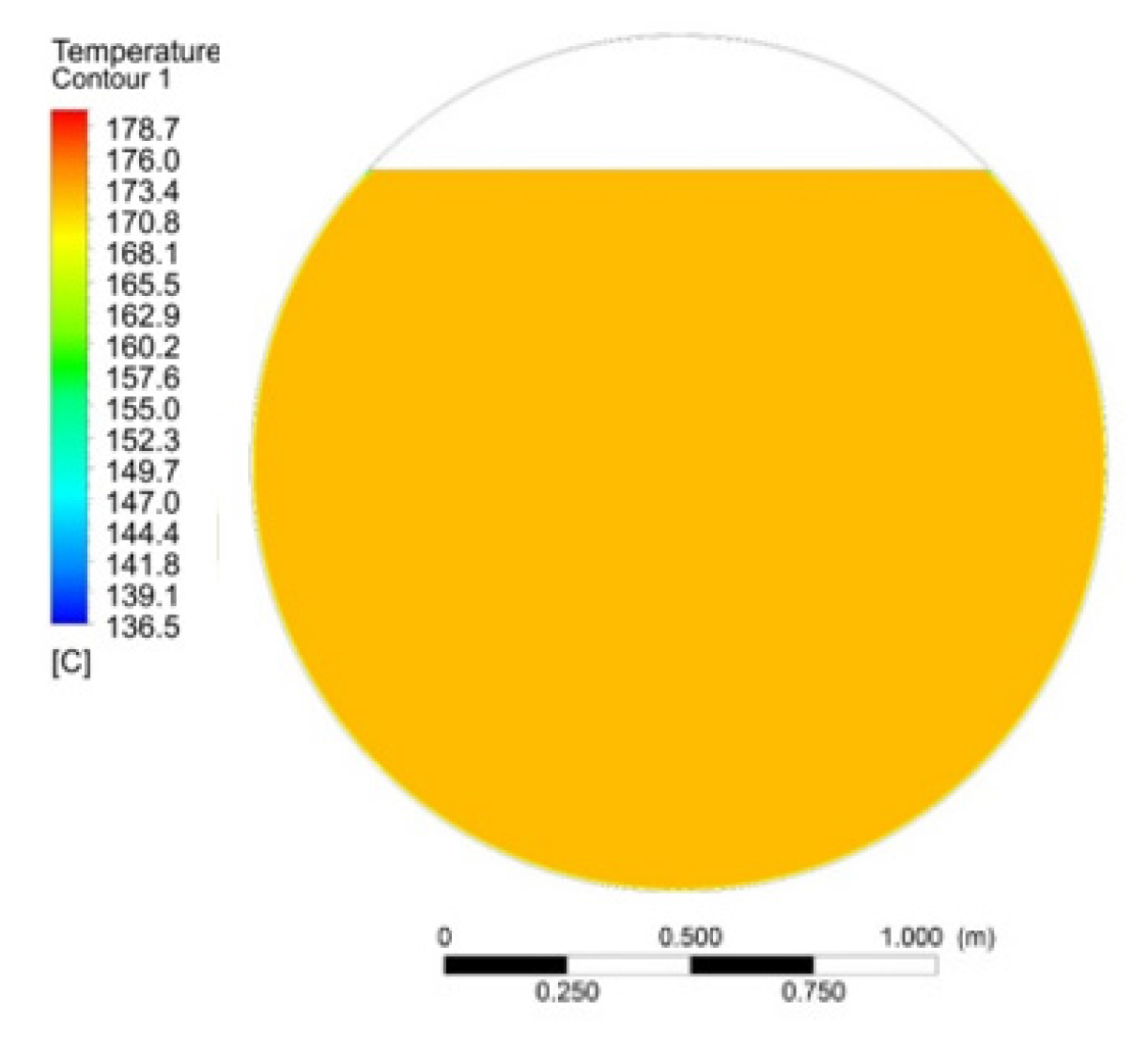
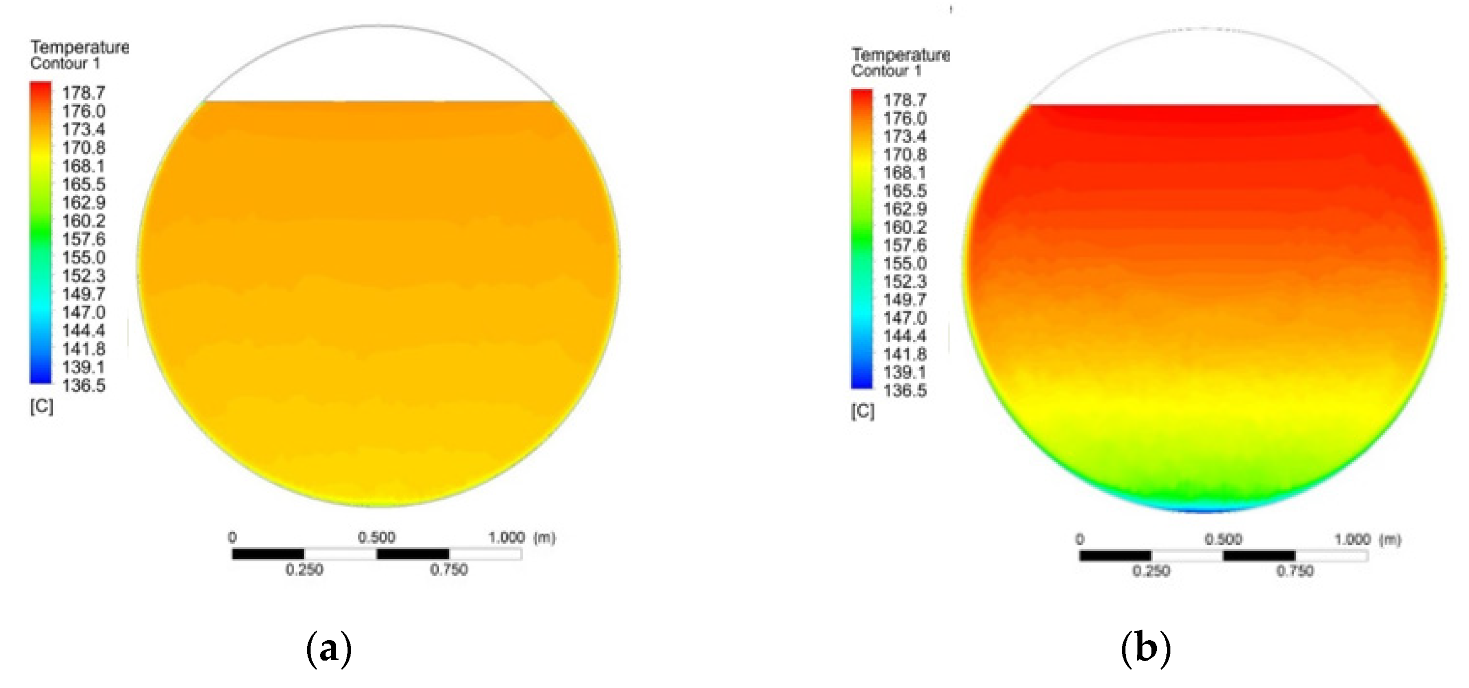
The numerical calculations showed that at a low dynamic viscosity (0.01 Pa·s), as shown in Figure 1, the temperature gradient along the tank height in its vertical axis after 60 h was negligible. With an increasing dynamic viscosity, the liquid circulation ceased, and after reaching the value of approximately 6 Pa·s, the liquid exhibited thermal layering (Figure 2a). In the case of a liquid with a dynamic viscosity of 100 Pa·s, the layering is significant, as is shown in Figure 2b. After 60 h of cooling, the liquid temperature difference along the tank height was as much as 42.9 °C (Figure 3). The lower temperatures at the bottom of the tank may even cause the transported liquid to solidify. With the low viscosities of 0.01 and 0.0003 Pa·s, the temperature difference was as low as 0.5 °C; as a result, the two curves overlap on the graph.

As presented above, at the dynamic viscosity of 100 Pa·s, the temperature difference along the liquid height was significant. The liquid temperature in the lower part of the tank dropped sharply as the colder liquid from the boundary layer flowed down along the tank circumference to the lower part of the tank. The largest temperature drop was observed within the height of 0.20 m from the tank bottom, whereas the temperature gradient was significantly smaller above this height (Figure 4).

At the viscosity of 0.01 Pa·s, the temperature along the tank height remained virtually unchanged, except for the temperature changes that were observed within the height of 0.024 m from the tank bottom (Figure 4). Above this height, the calculated temperature gradient approached zero. The thermal profiles for the remaining investigated values of dynamic viscosity were located between the curves of the maximum and minimum viscosity. See the curve for a viscosity of 6 Pa·s in Figure 4.

5. Identification of the Criterial Equation Parameters

Provided that the correlations between the dimensionless arguments in Equation (20) are power correlations, the equation is as follows:

$${\pi }_1=C·{\pi }_2^{z_2}·{\pi }_3^{z_3}·{\pi }_4^{z_4}·{\pi }_5^{z_5}·{\pi }_6^{z_6}$$

(21)

In the logarithmic coordinates, such a correlation is linear, as follows:

$$\ln {\pi }_1=\ln C+z_2·\ln {\pi }_2+z_3·\ln {\pi }_3+z_4·\ln {\pi }_4+z_5·\ln {\pi }_5+z_6·\ln {\pi }_6$$

(22)

The C constant and the individual exponents z₂ through z₆ were identified using multiple linear regression. The results of the numerical simulations were used as the input data for the regression. The numerical simulation revealed that the average temperature of the fluid decreased over time very slowly. Therefore, temperature values in the longer time intervals were used when setting the constant and the exponents. In 31 simulations, this interval was 5 h, while in 20 simulations, the interval was 2 h. For the total period of 60 h, 972 values of the average temperature were obtained. These temperatures were calculated for various times and various combinations of the relevant parameters. The ranges in which the individual parameters were changed are presented in Table 1 above.

The values of the constant and the exponents are listed in

Table 2. Parameters of the regression function.

Constant	Exponent
C	z2	z3	z4	z5	z6
5.349 × 10−1	1.080 × 100	9.638 × 10−1	3.880 × 10−3	8.740 × 10−2	4.990 × 10−2

. The coefficient of determination for the multiple linear regression represented 0.9978. The regression sum of squares was 958.83, and the residual sum of squares was 2.1096.

The long version of criterial Equation (18) is as follows:

$${\pi }_1=C·{\left(\frac{a·\tau }{d_{\mathrm{ch}}^2}\right)}^{z_2}·{\left(\frac{k·d_{\mathrm{ch}}}{\lambda }\right)}^{z_3}·{\left[\left(\beta ·(T_0-T_{\mathrm{a}}\right)\right]}^{z_4}·{\left(\frac{\nu }{a}\right)}^{z_5}·{\left[\frac{c_p·d_{\mathrm{ch}}^2·\left(T_0-T_{\mathrm{a}}\right)}{{\nu }^2}\right]}^{z_6}$$

(23)

The sought temperature T was calculated using the temperature simplex π₁, as defined by Formula (11), using the following equation:

$$T=T_0-\left(T_0-T_{\mathrm{a}}\right)·{\pi }_1$$

(24)

6. Discussion and Conclusions

The results of the numerical solution exhibited an excellent accordance with the results of the similarity model. Figure 5 shows a correlation between the T_mod, calculated using Formula (24), and the T_sim obtained from the numerical simulation. It may be described by a regression line with the slope approaching one, in particular 0.9997, at the reliability value (square power of the correlation index) R² = 0.9999. The standard deviation of the difference T_mod–T_sim for 972 pairs of values was 0.27 K, which represents 4.8% relative to the average simulated temperature.

The regression model was validated using the Student’s t-test and the f-test. A critical threshold for 972 pairs of values at the significance level of 0.05 was 1.962 according to the Student’s t-test distribution. The test criterion value 1.171 did not exceed this value; this means that the numerical model and the similarity model provided consistent results. The Fisher–Snedecor distribution F with 6 regression parameters and 972 − 6 = 966 degrees of freedom was used as the test criterion. As its value 1.9 × 10⁶ is much higher than the quantile value 2.58 of the Fisher–Snedecor distribution for the level of significance 0.05, the regression model is significant.

The model, Equation (21), represents a universal formula for expressing the correlation between the temperature of a cooling fluid and the transport duration. The ranges listed in Table 1 are subject to the formula that is applicable to all the combinations of values for the physical parameters.

The benefit of defining the mean temperature of a fluid in the form of a criterial equation, depending on the transport duration, is that it fills the gap between the partial analytical procedures applied in the field of heat and mass transfer, and flow. Therefore, it is not necessary to apply numerical methods to each tank with a different fluid in different boundary conditions and with different transport durations.

The created model may be used by carriers responsible for transporting fluids. By a simple programming of the Equations (20) and (21), for example, in an Excel document, it is possible to quickly identify how long a particular fluid with certain physical properties may be transported without the risk of solidification.