The Effect of Load Control on the Performance of Contra-Rotating Fans

Abstract

In recent years, few studies focused on adjusting the load distribution of contra-rotating fan (CRF) blades. To improve the overall performance of CRFs, we used a design code to build 32 sets of CRFs to determine the effects of three factors—the front and rear rotor load matching, the load distribution of each rotor and the axial distance between the rotors—on the total pressure rise and efficiency of CRFs using numerical calculations. The relationship between the CRF blades load and velocity components was theoretically analyzed using blade element analysis and the forward problem method. According to the performance curve, it can be concluded that the rear rotor (RR) is the key factor that determines the performance of CRFs. Through analyzing Mach number contours from different perspectives, the relationship between velocity and adjustment load was verified. Furthermore, the flow field characteristics for three specific CRFs were explored at the stall points, design points and choke points to reveal their flow mechanisms. This study provides a reference for the CRF blade design method.

1. Introduction

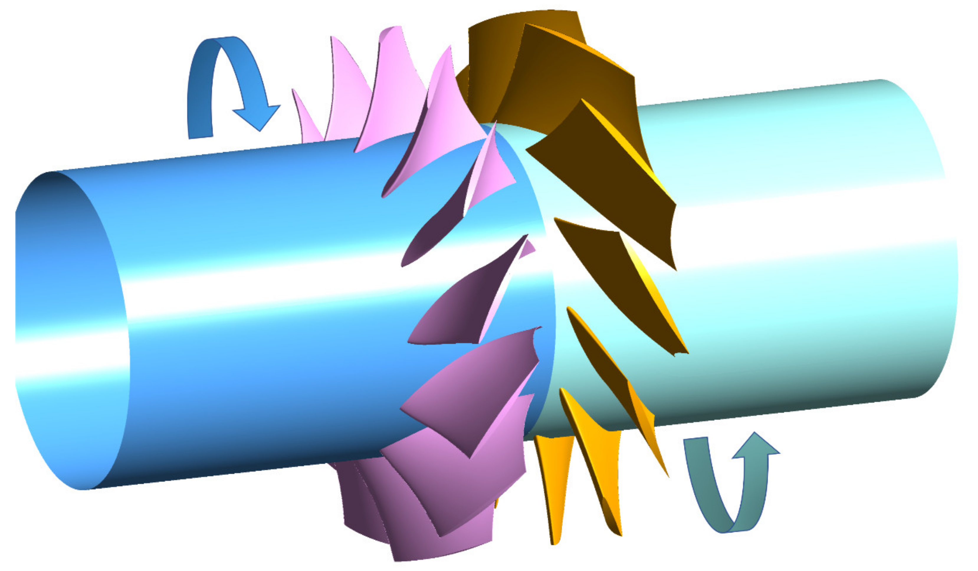
Since the concept of the contra-rotating fan (CRF) was proposed in the 1940s [1], scholars across the world have conducted extensive research on it. Compared with traditional fans, CRFs have the advantage of higher output performance with a more compact structure and smoother flow with a minor tangential velocity component at the outlet [2,3]. There are no vanes between the two-stage rotors of CRF, which makes CRFs benefit from it, but this is also the reason for their shortcomings; the inlet of the RR directly bears periodic interference from the front rotor (FR). The two rotors of a CRF can be controlled by two inputs, respectively. Therefore, in recent years, the optimization of the overall aerodynamic performance of CRFs was mainly based on adjusting the speed ratio of the two rotors to change their load matching.

Mohammadi and Boroomand [2] optimized the thickness of CRF rotor blades and found that the highest Mach number of flow medium was around 0.14 in the blade channel, meaning the flow medium could be considered an incompressible flow. They also performed a steady-state simulation of a CRF using the k-ε turbulence model, examining the influence of the axial distance and speed ratio of two rotors on the performance of the CRF and developing an optimized CRF model. Another low-speed CRF was studied by Sun et al. [3]. By measuring the change of flow velocity with respect to the different rotors rotating speed combinations, they found that the load distribution was similar when a CRF was operated at the maximum efficiency point for all of the speed combinations. Wang and Meng [4] established an electromagnetic fluid coupling model of a CRF, then analyzed its harmonic components combined with the fast Fourier transform algorithm. They also discussed the interaction and similarity in performance between rotors and motors to determine the best combination scheme of blade number of the two rotors, which would help the electromechanical resonance attenuation. Luan et al. [5] used the SST model to solve RANS (the Reynolds-averaged Navier–Stokes equations) to study the influence of the different rotating speed of the rotors matching on tip clearance flow behavior and the relationship between this and stall initiation. They concluded that the rotating speed change of the rear stage rotor (RR) of a CRF had no significant effect on the tip clearance flow field, while changes on the FR significantly influenced the stall boundary of the fan. Following this, they studied the relationship between different axial gaps and the unsteady influence on the CRF blade boundary layers [6], finding that, with the increment of the axial gap, the inhibition for separation in the RR boundary layers was weakened, since the rotor–rotor interaction of the CRF was weakened and the blade deformed. However, this had little effect on the radiation noise [7]. Ravelet et al. [8] redistributed the loads of a CRF load by applying three sets of speed ratios. By measuring and comparing the flow characteristics and unsteady characteristics of the three sets of CRFs, they concluded that, under the condition of keeping the rotor angular velocity of two stages approximately equal, redistributing the load of the FR to 60% and the RR to 40% could reduce the loss of the RR. Shahriyari et al. [9] reported a CRF post-stall transient theory, which could better predict the instability of a CRF. Besides, by studying the effect of different rotating speeds between rotors, which matched the stall and surge pattern, they concluded that, the higher the RR speed, the stronger the fan resistance to a surge caused by throttling. Ai et al. [10] improved the blocking margin and expanded the stability margin of CRFs by changing the speed of the RR to keep the power of the two rotors equal.

From the above analysis, it can be seen that changing the rotating speed ratio of the two rotors is one of the most efficient methods to enhance the performance of a CRF. However, fundamentally, the profile of the blades plays the most crucial role in the performance of a CRF, since the shape of the blades determines their load distribution. Few studies focusing on this aspect of CRFs have been carried out.

Vijayraj and Govardhan [11] reduced the incident loss of the FR and improved the power capacity and stall margin of the CRF by applying an axial sweep and tip chord sweep to the CRF rotors, which could rearrange the load distribution of the blades. They found that by sweeping the tip chord of the FR, the velocity distribution changed and the accumulation of low-energy fluid could be avoided.

There have been few experiments that have attempted to rearrange the profile of CRF blades to improve performance by controlling the load distribution of the blades, despite a blade profile being the fundamental element affecting the load distribution of a CRF.

Therefore, in this paper, using a CRF designed by the free vortex method as the baseline model, we built and simulated 32 sets of CRFs, with different blade profile results from the design code, by rearranging the load distribution from the hub to the shroud of each rotor blade. We also investigated the effect of the axial gap between rotors to validate previous findings. The effects on CRF performance and efficiency were studied and this provided ideas for the design method of a CRF. A flowchart of the article structure and related design code procedure is shown in Figure 1. The details of the baseline CRF are in Section 2. Its establishment process was calculated and predicted based on the primary method discussed in Section 3 and its performance was verified using the simulation method from Section 4. All explanations of abbreviations are listed in

Table A1. Nomenclature and related units for abbreviations.

CRF	Contra-rotating fan
CRF (F)	Contra-rotating fan (load control is applied to the FR)
CRF (R)	Contra-rotating fan (load control is applied to the RR)
D	Diameter, mm
FR	Front rotor
FR (F)	Front rotor (load control is applied to the FR)
FR (R)	Front rotor (load control is applied to the RR)
K	Circulation coefficient
LE	Leading edge
PS	Pressure side
$Q$	Volume flow rate, m3/s
$R$	Radius, mm
RR	Rear rotor
RR (F)	Rear rotor (load control is applied to the FR)
RR (R)	Rear rotor (load control is applied to the RR)
SS	Suction side
$T$	Temperature, K
TE	Trailing edge
$a$	Load control parameter
c	Absolute flow speed, m/s
$\overline{d}$	Hub/tip ratio
$i^{*}$	Stagnation enthalpy, J/kg
$p$	Static pressure, Pa
$p^{*}$	Stagnation static pressure or total pressure rise, Pa
$s$	Entropy, J/K
u	Rotational flow speed, m/s
w	Relative flow speed, m/s
$\eta$	Efficiency,
$\rho$	Fluid density, kg/m3
$\omega$	Angular speed, rpm

and

Table A2. Subscripts for abbreviation.

1, 2	Inlet, outlet of the rotor
h	Hub of the rotor
m	Mid-span of the blade
t	Tip of the blade
u	Tangential velocity component
z	Axial velocity component
zm	Axial velocity component at the mid-span

in Appendix A.

The procedure of the design code can be concluded as: First, the expected parameters of the design point are determined according to the design value required. Then, the overall size of the blade channel is calculated according to these parameters. The third step is to check the primary aerodynamic performance through empirical formulas. After that, motors are selected based on the expected efficiency and power. Next, the aerodynamic parameters of each element are calculated according to the design point parameters. According to the aerodynamic parameters, the profiles of airfoils are obtained and the establishment of three-dimensional models is completed. The performance of models is verified using the simulation method from Section 4 and feedback is received. The entire process is ended after several iterations until reaching the required value.

2. The Baseline CRF Model

The baseline model used in this paper was a CRF designed according to the free vortex design method. The basic design parameters of the CRF are listed in

Table 1. The baseline CRF design specification.

Characteristics	Value
Tip diameter (mm)	602
Hub/tip ratio	0.598
Tip clearance (mm)	1.5
Axial gap between rows (mm)	84.275
Rotational speed (rpm)	2950
Speed ratio (FR/RR)	1
Mass flow rate (kg/s)	9.144
Total pressure rise (Pa)	4860
Total pressure rise ratio (FR/RR)	1
Blade profile	NACA 65 series

. The load distribution of the FR and RR at the design point was equal, at 2430 Pa. Their rotational speed was identical, but in a counter-rotating direction, and their hub diameter and hub ratio were also identical. The blade profile in each element from the hub to the shroud was designed according to NACA-65 series cascade profiles experimental data from Mellor [12]. Their load distribution ensured better performance in low subsonic compressors. The blade profile data, calculated by the design code, are listed in

Table 2. The profile data of the baseline CRF.

	FR			RR
	Hub	Mid	Tip	Hub	Mid	Tip
Inlet relative flow angle (degrees)	37.19	28.84	24.41	23.08	21.32	19.53
outlet relative flow angle (degrees)	70.87	42	31.64	37.19	28.84	24.41
Solidity	1.37	1.13	1.02	1.36	1.13	1.02
Incidence angle (degrees)	2.5625	1.25	−0.0625	2.5625	1.25	−0.0625
Camber angle (degrees)	39.28	17.14	11.83	15.29	9.37	8.41
Stagger angle (degrees)	62.14	40.97	32.12	36.43	29.96	25.94
Length of the mean camber line (mm)	195.74	154.90	145.47	231.33	182.19	171.93

. It can be seen that the mean camber line, stagger angle and solidity increase non-linearly from the tip to the root along the radial direction of the blade. As shown in Figure 2, there are 13 blades in the FR and 11 in the RR, with a constant height blade channel.

3. Load Control Method

Previous research has shown that the distribution of velocity components is related to the load distribution [3,8,11,13,14]. However, due to the dynamic interference between the rotors without a guide vane in a CRF, the relationship between the velocity components and the load differs, compared to a traditional axial fan.

3.1. Velocity Triangle Analysis

First, it should be clarified that the complex three-dimensional flow of turbomachinery can be simplified and decomposed into two types of three-dimensional flow surface: S1 (blade to blade surface) and S2 (meridional surface). The blade element assumes that a blade is composed of elements in numerous S1 flow surfaces from the hub to the shroud. Therefore, the forward problem method, combined with the blade element analysis, was used to check the inlet and outlet velocity components of two rotor blades at the baseline CRF model design point, as shown in Figure 3. The load could also be differentiated into each S1 flow surface from the hub to the shroud, according to the rotating speed and performance parameters of the rotors at the design point. Then, the Euler equation was used to verify the relationship between velocity $c_u$ and load. Using the radial balance equation, the two rotors axial velocity components of the CRF in the S2 flow surface were related to the differentiated load in each S1 flow surface; this is analyzed in detail in Section 3.2. By redistributing the load for each blade of a CRF, the blade profiles were changed to control the velocity components, which could improve the performance of the CRF.

3.2. Relationship between Load and Axial Velocity Components

Owing to the complexity of the actual flow of a CRF, we made the following simplified assumptions to establish a design code for the three-dimensional flow field of a CRF:

• The flow is ideal gas and, since the maximum Mach number would exceed 0.3 at the RR, the compressibility of the flow should be taken into consideration;
• The flow is adiabatic and inviscid;
• The gravity of the flow can be omitted;
• The S1 flow surface is a series of cylindrical flow surfaces without radial flow $c_r=0$;
• The flow is axisymmetric $\frac{\partial }{\partial \theta }=0$.

On the one hand, from the simplified balance equation [12], the relationship between total pressure rise and axial velocity component along the radius can be obtained by:

$$\frac{1}{\rho }\frac{d{p}^{*}}{dR}=\frac{1}{2} \left[ \frac{1}{R^2} \frac{d{\left(R{c}_u\right)}^2}{dR}+\frac{d{c}_z^2}{dR} \right]$$

(1)

In addition, it can be obtained, with the Euler turbine equation [12]:

$$\frac{d{p}^{*}}{dR}= \left[ \rho \frac{d\left(u{c}_{2u}-u{c}_{1u}\right)}{dR} \right]$$

(2)

The swirl $c_u$ also relates to the total pressure rise. Therefore, by defining the circulation coefficient $K$, the relationship between $c_u$ and $R$ is determined as $c_u{R}^a=K$ [12]. The definition of $K$ is

$$K=\frac{p^{*}\left(3-a\right)\left(1-{\overline{d}}^2\right)}{2\eta \rho \omega R_t^{1-a}\left(1-{\overline{d}}^{3-a}\right)}$$

(3)

That is, by setting the value of a, the axial velocity distribution along the radius in the S2 flow surface and the load distribution in the S1 flow surface can be controlled.

Since the flow upstream of the FR at the entrance is swirl-free, that is, $c_{1u}=0$, the outlet axial velocity component of the FR is calculated by Equations (1)–(3), as follows:

$$c_{2z}^2=c_{2zm}^2+2K\omega \left(R^{1-a}-R_m^{1-a}\right)+\frac{1-a}{a}{K}^2\left(R^{-2a}-R_m^{-2a}\right)$$

(4)

Among which,

$$\begin{gathered} R_m=\frac{1}{2}\sqrt{\frac{D_t^2+d_h^2}{2}} \\ {c}_{2zm}=\frac{4Q}{\pi \eta D_t^2\left(1-{\overline{d}}^2\right)} \end{gathered}$$

In terms of the axial velocity component distribution of an RR, its inlet value is equal to the FR outlet, when its outlet value is designed to be equal to the FR inlet. That means the circumferential velocity component of the flow at the RR outlet is wholly eliminated at the design point.

To ensure the symmetry of load distribution in each S1 flow surface, the sum of the total pressure rise of the FR and RR elements should be equal to the baseline model, which is 4860 Pa. Therefore, the RR load at certain elements should be reduced as much as the value is increased by the FR for the same elements. Thus, when the load control is applied to the RR, the FR outlet axial velocity can be calculated as follows:

$$c_{2z}^2=c_{2zm}^2+2K\omega \left(R^{a-1}-R_m^{a-1}\right)+\frac{a-1}{2-a}{K}^2\left(R^{2a-4}-R_m^{2a-4}\right)$$

(5)

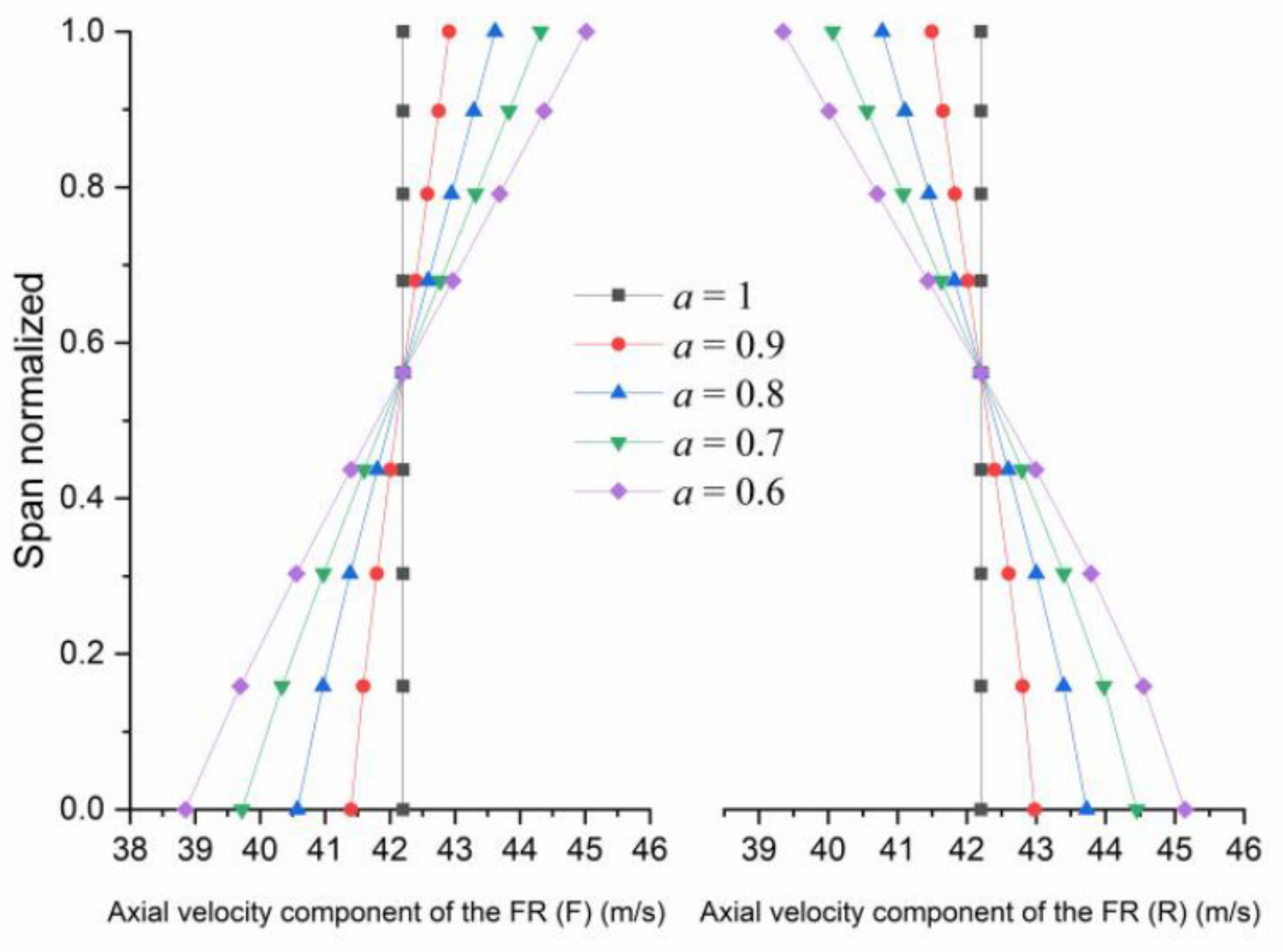
The axial velocity distribution at the FR TE for these two situations, as predicted by design code, is shown in Figure 4. By controlling the FR, the axial velocity components above the mid-span can be increased evenly. Thus, the smaller the value of a, the bigger the increment. The components below the mid-span can be decreased evenly, as shown on the left half of Figure 4. When the load control is applied to the RR, the situation is reversed, as shown on the right half of Figure 4.

Through the above analysis, it can be concluded that the load and axial velocity components are positively correlated. Therefore, we used this code to predict the distribution of the axial velocity component in the S2 flow surface to guide the blade profile design of the blade element in each flow surface to achieve a reasonable load distribution.

4. Numerical Simulation

In this paper, 32 sets of CRFs were built and analyzed. Time and financial constraints precluded the use of metal models, so numerical simulation methods were adopted.

A three-dimensional numerical simulation was performed with the ideal gas medium. To improve the calculation efficiency, periodic boundary conditions were adopted, which reduced the calculation time. First, the simulation was conducted on the case study of a NASA Rotor 67 to evaluate the validity of the method. Then, the simulation was performed using the baseline CRF model to verify the effectiveness of the design code of the CRF.

4.1. Numerical Model Validation

To verify the effectiveness of the simulation setup method, the case of the NASA Rotor 67 was selected to analyze the flow medium in transonic conditions. Figure 5 shows the three-dimensional model of the NASA Rotor 67 and

Table 3. NASA Rotor 67 specification.

Characteristics	Value
No. of blade	22
Inlet hub/tip ratio	0.375
Exit hub/tip ratio	0.478
Tip clearance (mm)	1.01
Rotational speed (rpm)	16043
Mass flow rate (kg/s)	33.25
Pressure ratio	1.63

shows its design parameters [15].

The calculated performance and efficiency curves are shown in Figure 6. The trend and accuracy proved that the numerical simulation method could accurately predict the steady-state performance curve; thus, it was used for the following research. The detailed setting method is discussed in Section 4.2.

4.2. Simulation of the Baseline CRF Model

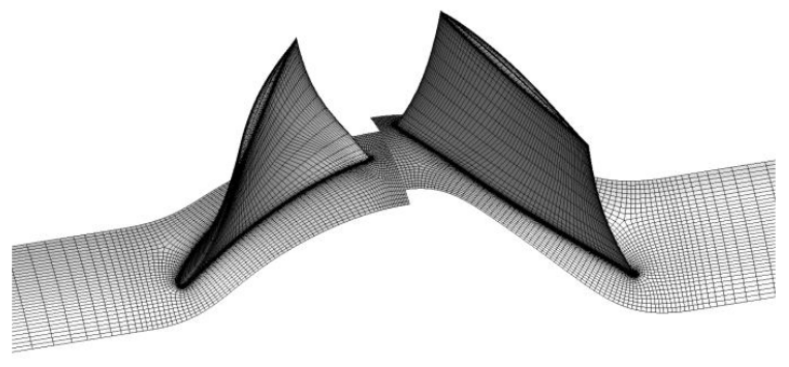
The automatic topology optimization grid division of the baseline CRF 3D model was completed using the TurboGrid module on the ANSYS Workbench software. Y+ was controlled within 20 to fit for RNG k-ε turbulence model and the grid sensitivity analysis result is shown in

Table 4. Grid sensitivity analysis for the baseline CRF.

FR Surrounding Nodes	RR Surrounding Nodes	Total Pressure Rise (Pa)	Relative Change Rate (%)	Total Pressure Efficiency	Relative Change Rate (%)
117,927	123,048	4920	-	0.890	-
161,611	187,332	4895	0.00515	0.894	0.00449
212,895	218,649	4879	0.00328	0.896	0.00223
314,387	319,163	4876	0.00062	0.897	0.00112
427,469	400,048	4874	0.00041	0.898	0.00111

. The total pressure rise and efficiency calculated by the third and fourth groups of grids were similar and tended to be stable, so the third group of grids was adopted here. The grid overview is shown in Figure 7, where the inlet domain of the FR and outlet domain of the RR adopted the H-grid, while a symmetric topology was produced at the round LE and TE for the FR and RR blade passage.

A CFX solver was then selected to solve the compressible steady RANS equations of the model. Due to the large reverse pressure gradient in the RR channel, the RNG k-ε turbulence model was chosen to close the equation. Since a function form was used to replace the constant coefficients in the original k-ε turbulence model that was used in the Rotor 67 case, the RNG k-ε turbulence model improved the simulation accuracy. A similar accuracy could be obtained using the RNG k-ε turbulence model as the SST model in terms of overall performance, yet with less demand on computing resources and refining grids in the boundary layer. It is difficult, for this CRF model, to achieve residual convergence at 10⁻⁶ with the SST turbulence model, while it is easier to realize this with the RNG k-ε turbulence model.

The flow medium was the ideal gas and the inlet boundary conditions were 298.15 K and 1 atm. The mass flow rate was set at the outlet boundary conditions to determine the calculated working conditions. The periodic boundary conditions were used in the circumferential direction, which can significantly shorten the calculation time. An adiabatic and no-sliding-wall condition was adopted for all related walls. The interface between rotors adopted a mixing plane. In terms of the advection scheme, a high-resolution scheme was chosen to guarantee conformity with the physical value. An upwind algorithm was adopted to solve the turbulence equation and accelerate convergence. With a conservative estimated length scale from the overall size of the calculating model, the timescale was calculated automatically, based on the related boundary conditions. The time scale factor was set as 1. A double precision algorithm was used for the calculation of the solver to ensure calculation accuracy of the two relatively rotating regions. The calculation ended until residuals reached 10⁻⁶.

The simulated total pressure performance and efficiency curves of the baseline CRF are shown in Figure 8. From the overall review, because the performance curve trends of the full stage and RR coincide, the overall performance of the CRF was determined by the performance of the RR. The flow rate at the highest efficiency point was lower than the design point and the output power of the RR was slightly larger than the FR at that point. Moreover, at the near stall point, as the mass flow rate decreased, the slope of the performance curve of the RR and the full stage remained consistent, gradually changing from a negative to a positive slope. At the choke point, because the RR reached zero first, the overall performance curve coincided with the performance curve of the FR. The performance curve of the FR maintained a constant slope. At the design point, the simulation result of the full stage total pressure rise differed by 0.39% from the expected design value, meaning the code fully met the requirements. The calculated results at the design points obtained by the simulation are shown in

Table 5. CFD results of the baseline CRF at the design point.

Characteristics	Value
Total pressure rise in the full stage (Pa)	4879
Total pressure rise in the FR (Pa)	2441
Total pressure rise in the RR (Pa)	2441
Mass flow rate (kg/s)	9.144
FR shaft power (W)	20,569.96
RR shaft power (W)	21,432.17
Total pressure efficiency in the full stage	0.89633
Total pressure efficiency in the FR	0.91568
Total pressure efficiency in the RR	0.87884

. As the efficiency of the RR was lower than the FR, the shaft power of the RR was higher than the FR, when their output power was equal.

5. Factor Experiment

A series of experiments were performed to study the effects of the load matching of the FR and RR, the load distribution of each rotor and the axial gap between the rotors on the total pressure. We did not perform a comparative analysis related to efficiency, because the difference in the efficiency results between experiments was too small.

First, the relationship between each factor and the total pressure was investigated by arranging experiments on 32 sets of CRFs built up from different combinations of the three factors. Simulations were carried out on each CRF at the same mass flow rate as the design point of the baseline CFR. Following this, two sets of combinations of the three factors were selected, which could cause the design points to move to the highest and lowest performance region; this is discussed in Section 5.1. The overall performance curve of these two models was then calculated to determine the design points, stall points and choke points, which were required for the comparative analysis.

Here, the “value a” that was mentioned in Section 3.2 was set to control the load matching between the FR and RR, as well as each rotor load distribution. The letter in the back bracket is used to indicate the rotor to which the load control is applied. Figure 9 shows the code results of controlling the blade load by setting value a to 0.9, 0.8, 0.7 and 0.6. Obviously, the smaller value a is, the greater the load variation of a single rotor blade from the hub to the shroud. In detail, the code predicted that the implementation of load control on the FR would uniformly increase the load above the mid-span of the FR and reduce the load below the mid-span. The load on the top of the RR would decrease accordingly and the situation at the root would be the opposite, as shown in the left half of Figure 9. The right half of Figure 9 shows that, when the load control is implemented on the RR, the result is contrasting. The total pressure rise from the hub to the shroud of the rotor designed by the free vortex design method was constant, at both the FR and RR. The axial distance between the FR trailing edge (TE) and RR leading edge (LE) at the blade mid-span was considered, to study its effect on the load distribution more comprehensively, in combination with the other two factors. Specifically, when the axial gap between the rotors was defined as 0.45, the value of the distance was 0.45 times the sum of the FR and RR chord length at the mid-span. The levels of each factor used in the experiments are shown in

Table 6. Levels of each factor.

Level	Factors
	Value a	Axial Gap between Rows	Controlled Rotor
1	0.9	0.5	FR
2	0.8	0.55	RR
3	0.7	0.6	-
4	0.6	0.65	-

.

5.1. Effect of Value a

Experiments were carried out at fixed axial gaps of 0.5, 0.55, 0.6 and 0.65 to investigate the relationship between value a and the performance of the CRF rotors. It should be noted that the roots of the two rotors interfere with each other when value a is too small. Since the axial gap is defined at the mid-span, while the distance between the FR TE and the RR LE is shortest at the hub, as shown in Figure 10, and the roots of the two rotors are already very close, they would interfere strongly with each other, if value a were to decrease. Thus, the minimum value a was limited to 0.6.

Figure 11a shows that when the load control is performed on the FR, the difference compared to the baseline CRF total pressure increases with the increment of value a. Thus, the difference has a minimum value when value a equals 0.6. In addition, the RRs are the main contributor to the total pressure difference. The FRs are almost unchanged.

It should be explained that, with a smaller difference, it is more likely that the design point of that set of CRF is in the low-performance region. When the difference value is larger, the design point of that set of CRF is more inclined to be in the high-performance region.

When the load control is performed on the RR, the difference value compared to the total pressure of the baseline CRF decreases with the increment of value a, as shown in Figure 11b. Thus, the difference has a maximum value when value a is 0.6. Similarly, the RR is the main contributor to the total pressure difference, while the FR is almost unchanged.

5.2. Effect of the Axial Gap between Rotors

When studying the effect of the axial gap on the total pressure rise, value a was fixed. It can be seen, from Figure 12a, that, when the load control is applied to the FR, the difference with the baseline CRF total pressure decreases with the increment of the axial gap. However, when the load control is applied to the RR, as shown in Figure 12b, there is the same trend as when FRs are controlled, except at a = 0.6. However, RRs are clearly still the main contributor to the total pressure difference. The FRs remained almost unchanged.

In addition, when controlling the variables, even if only value a or the axial gap are changed, the degree of freedom of the airfoil itself and the flow field cannot be guaranteed to have only one degree of freedom and the nodes of each model also differ. Therefore, it can be seen, from Figure 11 and Figure 12, that there are around four points among the 48 data points that are inconsistent with the apparent primary trend.

6. Results

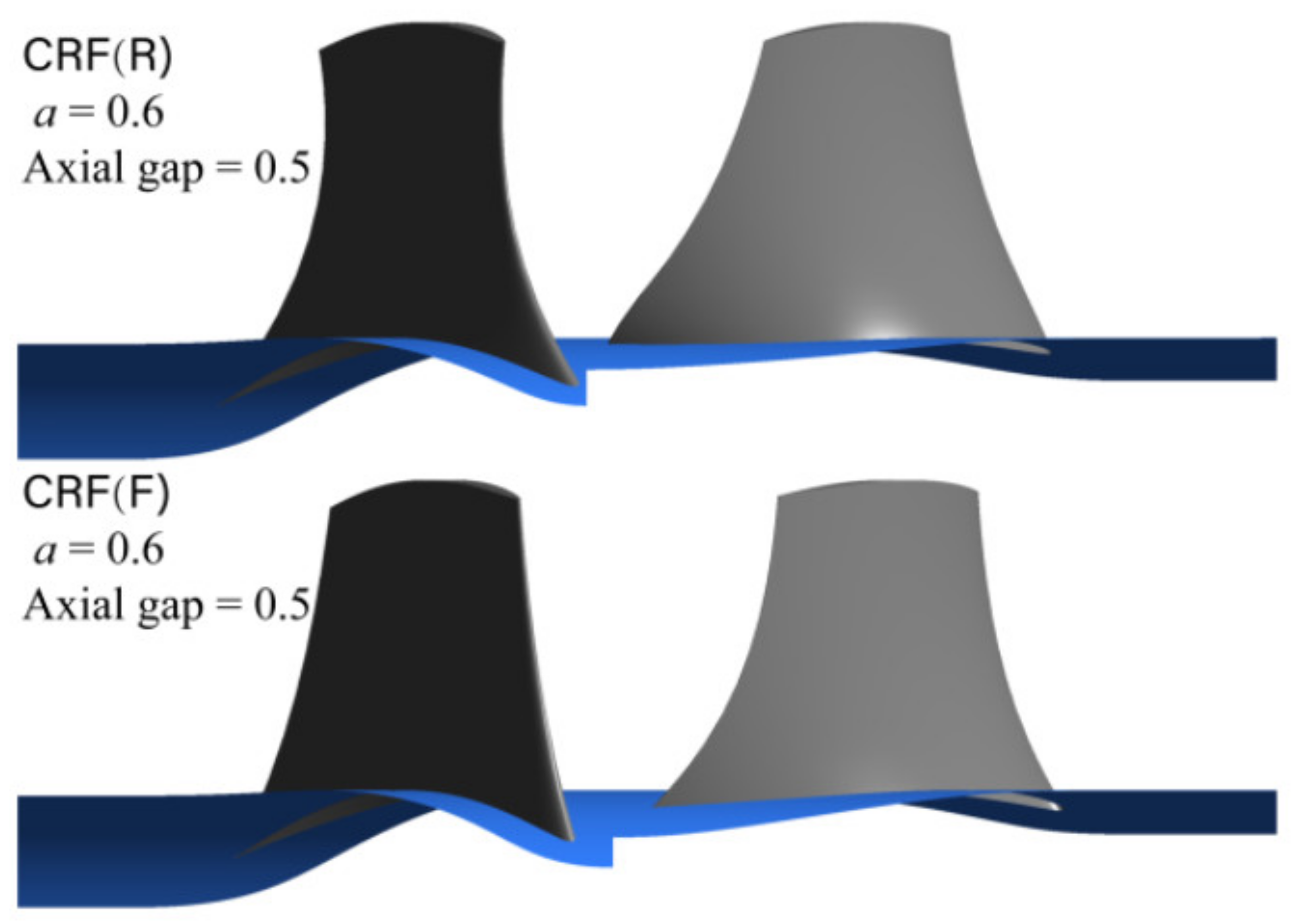
Two specific combinations were selected from the 32 sets of CRFs that could lead their design points to move to the highest and lowest performance regions, enlarging the differences with the baseline CRF as a result. The overall performance curves of these two combinations were then calculated:

• value a = 0.6, axial gap = 0.5, while the load control was applied to the FR. Profile data of blades results from the design code are shown in

  Table 7. Profile data of blades of CRF (F).

  	FR			RR
  	Hub	Mid	Tip	Hub	Mid	Tip
  Inlet relative flow angle (degree)	37.19	28.84	24.41	20.48	21.36	21.10
  outlet relative flow angle (degree)	63.54	42.11	34.16	37.19	28.84	24.41
  Solidity	1.34	1.10	1.01	1.35	1.13	1.02
  Incidence angle (degree)	2.5625	1.25	−0.0625	2.5625	1.25	−0.0625
  Camber angle (degree)	24.76	17.42	15.65	18.88	9.32	5.96
  Stagger angle (degree)	57.67	41.10	33.99	35.62	29.97	26.28
  Length of the mean camber line (mm)	195.74	145.75	145.47	231.33	181.25	171.93

  ;
• value a = 0.6, axial gap = 0.6, while the load control was applied to the RR. Profile data of blades results from the design code are shown in

  Table 8. Profile data of blades of CRF (R).

  	FR			RR
  	Hub	Mid	Tip	Hub	Mid	Tip
  Inlet relative flow angle (degree)	37.19	28.84	24.41	25.76	21.27	18.00
  outlet relative flow angle (degree)	78.14	41.82	29.15	37.19	28.84	24.41
  Solidity	1.39	1.15	1.02	1.27	1.01	0.98
  Incidence angle (degree)	2.5625	1.25	−0.0625	2.5625	1.25	−0.0625
  Camber angle (degree)	47.86	16.85	8.09	11.61	9.73	10.81
  Stagger angle (degree)	66.42	40.82	30.25	37.27	30.08	25.60
  Length of the mean camber line (mm)	195.74	158.63	145.47	231.33	145.19	171.93

  .

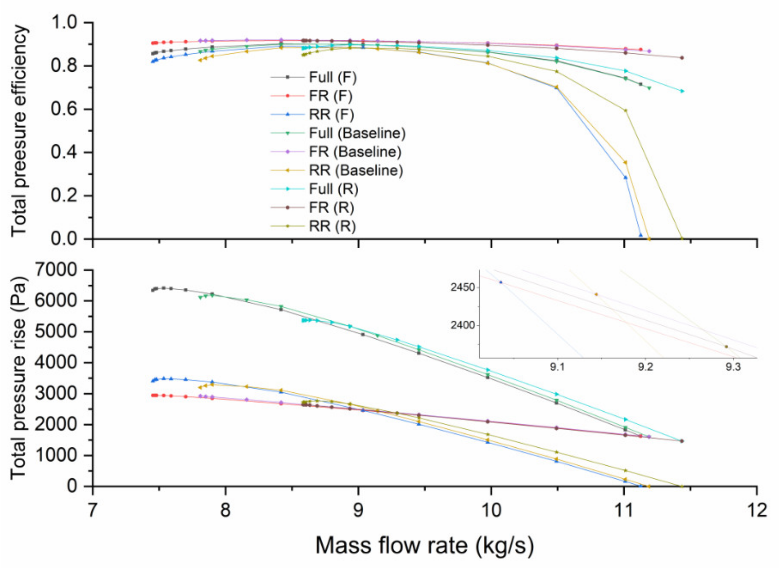
Results of the simulation are shown in Figure 13. The FR performance curves of the three sets of CRFs coincide. Similar to the overall performance shown in Figure 8, the RR performance was still the key determinant of the overall performance of each group of CRFs. Through the analysis of the overall performance of the three sets of CRFs, it can be seen that the load control of the FR can move its design point to the low-performance region but inhibit the occurrence of the stall; this is analyzed in Section 6.2. Furthermore, the high-efficiency operational area is enlarged [16]. The load control of the RR can move the design point to the high-performance region and improve the flow capacity and efficiency of the RR near the choke point, but the high-efficiency operational area is shortened.

6.1. Analysis at the Design Points

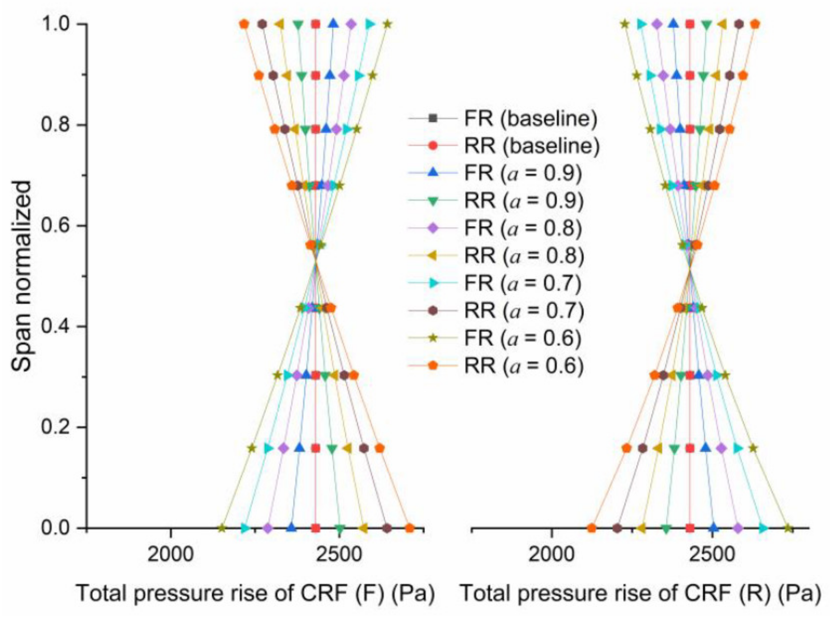
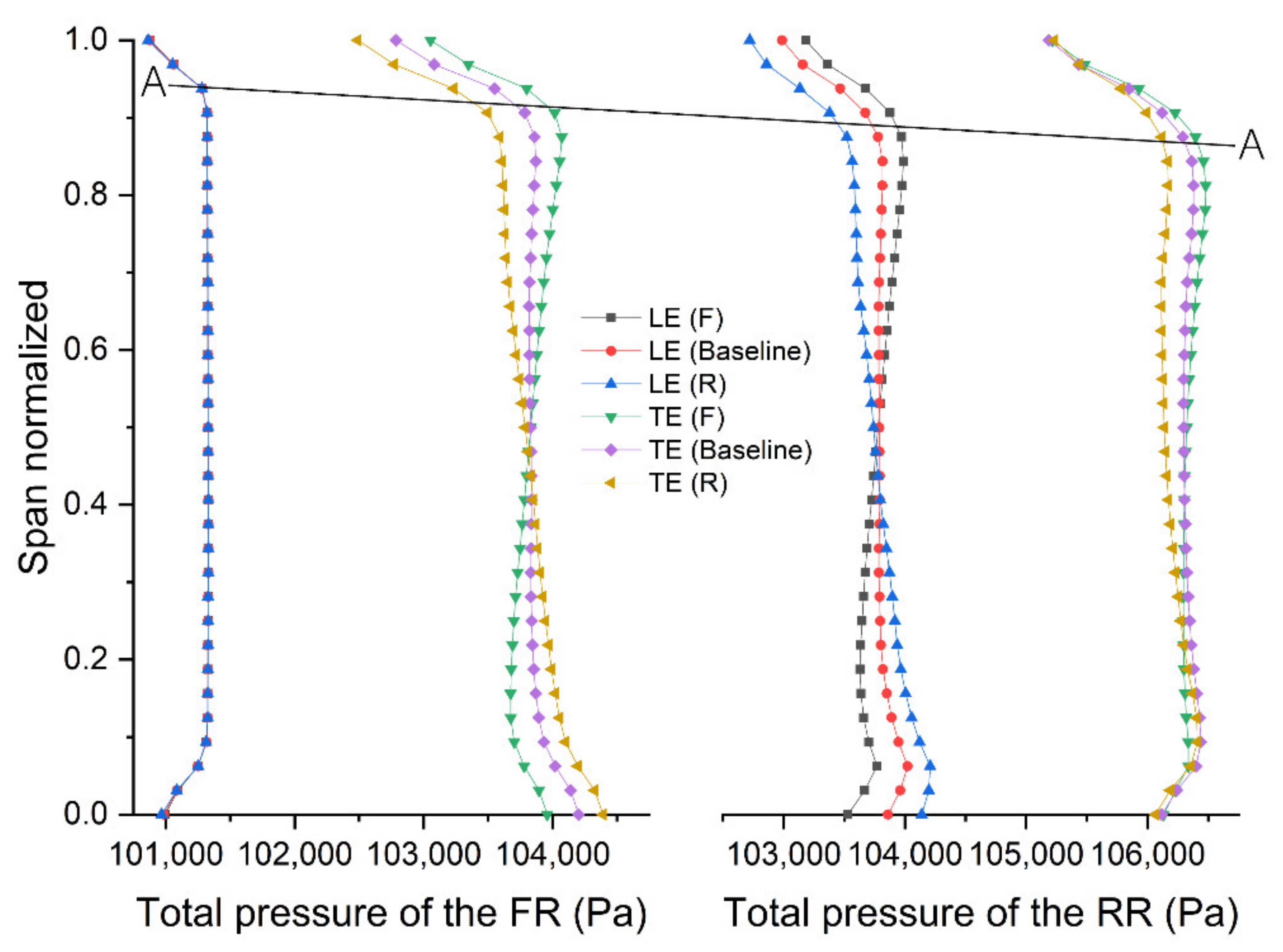
Figure 14 shows the simulation results at the design point and the total pressure trends coincide with those in Figure 9. As shown in the left half of Figure 14, when the load control is applied to the FR, the total pressure at the root of the FR is reduced, while the total pressure at the top is increased. The RR situation is the opposite and complementary to the FR, as shown in the right half of Figure 14. The total pressure distribution is relatively even at the RR TE. On the other hand, when the load control is applied to the RR, the total pressure at the FR root increases and the total pressure at the top of the FR decreases. The situation of the RR is also complementary to the FR and the total pressure distribution of the RR at the TE is relatively uniformly distributed.

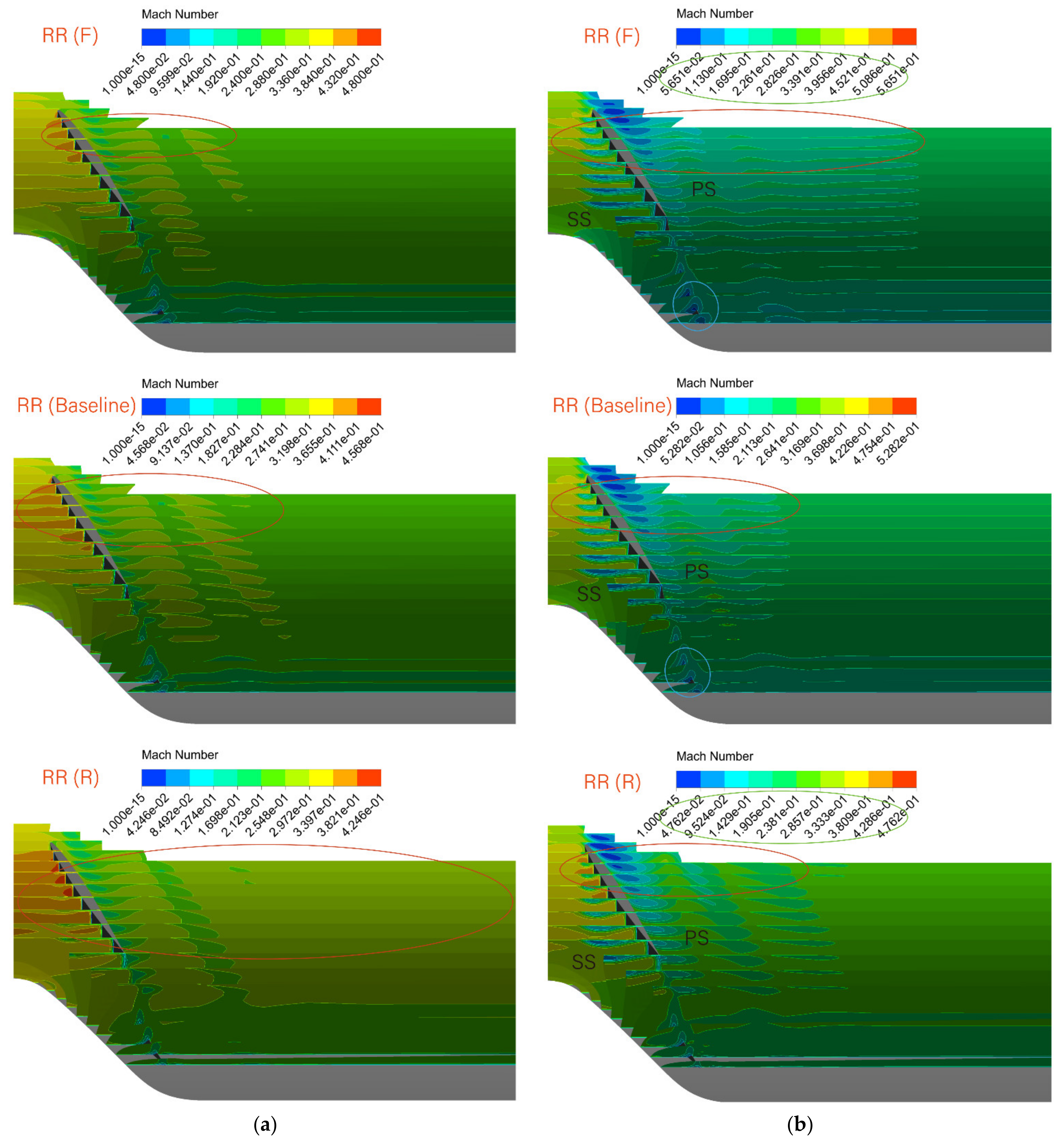
Correspondingly, from the Mach number contour shown in Figure 15a of the three models under the design point conditions, it can be seen that the high Mach number area at the top of the RR (F) is reduced relative to the RR (baseline). In contrast, the high Mach number area at the top of the RR (R) increased relative to the RR (baseline). The three models all exhibit corner separation at the TE of the FR due to the accumulation of low energy flow at the root of the FR, shown in the red circles in Figure 16a.

In Figure 14, the total pressure distribution in front of the FR LE is evenly distributed in the radial direction, but near the wall shroud and hub, because the wall is a non-sliding wall, the speed reduces, as it approaches the wall, and the total pressure decreases accordingly. After the tip clearance flows through the tip of the FR, the total pressure is further reduced at the TE. At the root, the fluid velocity increases, due to the suction effect of the RR on the FR and the total pressure increases. As the tip of the RR is rotating at the highest relative velocity in the entire channel, the flow loss is relatively significant, due to the relatively high speed. Coupled with the periodic interference upstream, the loss is further increased and deteriorated, the total pressure is further reduced and the affected area continues to expand from the FR LE to the RR TE, as shown in the A–A line in Figure 14. However, due to periodic disturbances upstream and the interaction of the boundary layer of the hub end wall, the loss of total pressure is also produced at the root of the RR.

It can also be seen, from Figure 15a,b, that the overall velocity reduces from the RR (F) to the RR (baseline) and, further, to the RR (R). This occurs because the load control of the FR makes the accelerating process of the upstream area of the RR stronger than the RR. However, the high Mach number area at the top of the RR gradually expands, because the load control of the RR can increase the velocity of the fluid at the top of the RR, thereby driving the velocity of the entire flow channel.

Similarly, it can be seen, from Figure 16a,b, that the high Mach number area of each region gradually expands, starting from the shroud spreading to the hub and this effect is greater going from the RR (F) to the RR (baseline) and the RR (R). Hence, the low-energy fluid area also gradually decreases in size.

However, in Figure 17a,b, going from the RR(F) to the RR (baseline) and the RR (R), the distribution of the Mach number of the FR remains unchanged, while the high Mach number area of RR gradually expands from the shroud to the entire flow channel.

6.2. Analysis at the Stall Points

When the mass flow of the three models is reduced from the design point to close to the stall boundary, the fluid acceleration at the top of the RR (R) can inhibit the diffusion of the low-energy fluid area (red circles in Figure 15b). However, for the RR (F), the fluid flowing through the top of RR (F) is the fluid that accelerated in the FR (F) region and the inertial velocity is relatively high, as shown in the green circles in Figure 15b. While the fluid at the top of the RR (R) begins to accelerate, this relatively low-speed fluid faces a larger pressure gradient than the front rotor during this acceleration process, so it is more likely to stall. Therefore, the overall performance difference shown in Figure 13 at the stall points is produced. Furthermore, it can be concluded that the characteristics of RR have the greatest influence on CRF performance, which is consistent with the conclusions reached by other researchers [6,17,18,19].

According to Figure 15b and Figure 16b, it can be seen that the stall phenomenon of the three models starts at the RRs.

On the pressure side, around the top of the RR (baseline) LE, the accumulation of low-energy fluid produced by the tip clearance flow increases (blue circles in Figure 16b). As RR (F) and FR (F) need to complement each other in terms of total pressure, the amount of work performed at the top of the RR (F) decreases and the fluid coming from the FR (F) begins to decelerate in this area. Combined with the influence of tip clearance flow, the radiation range of low-energy fluid becomes larger in the same area.

With regard to the suction side, around the root of the RR (baseline) TE, corner separation occurs due to the large pressure gradient from the blade channel, which results from the low-energy fluid accumulated in the boundary layer between the hub and blade root (red circles in Figure 16b and blue circles in Figure 15b). The RR (R) reduces the pressure gradient in this region by reducing the work performed at the blade root, thus inhibiting the corner separation.

6.3. Analysis at the Choke Points

When the flow rate increases from the design point to the choke point, the pressure gradient of RR is not as large as the stall point and the acceleration process is easier to achieve. Therefore, RR (R) is filled with high Mach number fluid in the blade channel at the choke point, as shown in the blue circles in Figure 17a,b, which leads to the increase in the flow capacity of RR (R) at the choke point, as shown in Figure 13 at the choke points.

7. Conclusions

In this paper, blade element analysis and velocity triangle methods were chosen to calculate and analyze the relationship between the load distribution and velocity components of CRF blades. The load distributions of two rotors of CRFs were controlled separately by changing the profile of the blades. We then used the NASA 67 Rotor and the baseline CRF model as the research objects to establish the settings of the numerical simulation for the CRF. The design method code was then demonstrated to be valid. Finally, the effects of load matching between the front and rear rotors, load distribution of each rotor and axial gap between the rotors on the total pressure rise and efficiency of the CRF were studied by building up and calculating 32 sets of CRFs. The conclusions are as follows:

• The entire stage performance curve coincides with the RR while the FR remains almost unchanged, no matter how the load distribution changed in the experiments. The characteristics of the RR are key to overall CRF performance.
• The CRF (F) can move its design point to the low-performance region but inhibit the occurrence of the stall and enlarge the high-efficiency operational area. The CRF (R) can move the design point to the high-performance region and improve the flow capacity and efficiency of the RR near the choke point, but the high-efficiency operational area is shortened.
• By recreating the blade profile results from an increasing total pressure along the blade span at the specific area, a high Mach number area was shown to enlarge the region, which could reduce the influence of the low energy flow from the blade tip clearance and the end wall around the blade root. Reducing the amount of work performed by the RR at the specific area which encounters a more significant pressure gradient could help inhibit the separation observed.