Article

A Novel Kinetic Modeling Framework for the Polycondensation of Sugars Using Monte Carlo and the Method of Moments

by
Dimitrios Meimaroglou
1,*,
Sandrine Hoppe
1 and
Baptiste Boit
2
1
Laboratoire Réactions et Génie des Procédés, Université de Lorraine, CNRS UMR7274, LRGP, F-54000 Nancy, France
2
ROQUETTE Frères, 62136 Lestrem, France
*
Author to whom correspondence should be addressed.
Processes 2021, 9(5), 745; https://doi.org/10.3390/pr9050745
Submission received: 15 March 2021 / Revised: 12 April 2021 / Accepted: 17 April 2021 / Published: 22 April 2021
(This article belongs to the Special Issue Advanced Modeling of Biomanufacturing Processes)

Abstract

:
The kinetics of the hydrolysis and polycondensation reactions of saccharides have made the subject of numerous studies, due to their importance in several industrial sectors. The present work, presents a novel kinetic modeling framework that is specifically well-suited to reacting systems under strict moisture control that favor the polycondensation reactions towards the formation of high-degree polysaccharides. The proposed model is based on an extended and generalized kinetic scheme, including also the presence of polyols, and is formulated using two different numerical approaches, namely a deterministic one in terms of the method of moments and a stochastic kinetic Monte Carlo approach. Accordingly, the most significant advantages and drawbacks of each technique are clearly demonstrated and the most fitted one (i.e., the Monte Carlo method) is implemented for the modeling of the system under different conditions, for which experimental data were available. Through these comparisons it is shown that the model can successfully follow the evolution of the reactions up to the formation of polysaccharides of very high degrees of polymerization.

1. Introduction

Saccharides are biomolecules of great importance to our society, displaying significant market potential for several industrial sectors, such as cosmetics, pharmaceutics and food-related products. Saccharides of low degree of polymerization (DP), such as C5 and C6 monosaccharides, are typically obtained via the hydrolysis of starch or lignocellulosic biomass. These may be subsequently converted to glucose syrup, maltodextrin, polyols, organic acids, biofuels or other platform chemicals, such as fructose, sorbitol, citric acid, furfural, 5–(hydroxymethyl) furfural (HMF), formic acid and levulinic acid [1,2,3,4,5,6]. The hydrolysis of starch or lignocellulosic biomass can be carried out in acidic conditions or via the use of enzymes, with each route presenting different advantages and drawbacks in terms of the selectivity and the productivity of the process [7,8]. More precisely, in the presence of acid catalysts, several side-reactions may occur, in parallel to the hydrolysis of the sugars, such as decomposition and polymerization reactions. The polymerization reactions, which are also known as reversion reactions, are considered undesirable as they consume the monosaccharides to form disaccharides or low-DP oligosaccharides. However, under strict control of the humidity levels of the reaction medium, the polymerization of monosaccharides can be utilized for the synthesis of natural-origin products, presenting a direct interest to the food, nutrition and health industrial sectors.
The polycondensation of sugars under controlled temperature and humidity, in order to achieve sugars of high degree of polymerization, has been a subject of research interest since the early 50’s and the pioneering works of [9,10] and later [11]. A clear industrial interest has also been expressed very early for the synthesis of the so-called polyglucoses (or polydextroses), via the anhydrous melt polymerization of glucose and sorbitol in the presence of acid catalysts [12,13]. These reports have clearly shown the importance of several factors on the productivity and the quality indexes of the produced polysaccharides. More precisely, they have demonstrated that the type and concentration of the acid catalyst displays a direct effect on the presence of degradation side-reactions while the effective elimination of the water produced during the polycondensation reactions is crucial to achieve high degrees of polymerization by limiting the rate of hydrolysis [10]. Since then, several studies have been carried out in an attempt to better understand these reactions, either in view of suppressing them from the hydrolysis system as undesirable side effects, either in the framework of better controlling the characteristics of the produced polysaccharides within an optimized biorefinery viewpoint [14,15,16,17].
Mathematical modeling is a tool that has been traditionally implemented to describe the evolution of reactive systems and, in this sense, contribute to the understanding of the underlying phenomena (i.e., in the case of phenomenological models) and/or provide a predictive capability on key indexes of interest, in terms of the process conditions. Given the complexity characterizing the reactive system of biomass hydrolysis, several studies have proposed different reaction schemes in an attempt to encompass the various reaction routes leading to the observed variety of produced saccharides. One of the first kinetic models to be published for the hydrolysis of cellulose under dilute acidic conditions was that of [18], already in 1945. Since then, many new studies have been reported that modify the proposed kinetic scheme either to extend its application to a wider range of conditions or to focus on specific reaction routes and products (e.g., the decomposition reactions) [8,19,20,21,22,23,24]. However, in most of these studies, the polymerization reactions are commonly considered again as side reactions resulting only in oligosaccharides, on the basis of oversimplified kinetic schemes. For example, ref. [22] studied the reaction kinetics of glucose in mildly acidic aqueous solutions, under different temperatures and glucose concentrations. In that study, the different disaccharides (i.e., in terms of the type of glycosidic bond), as well as various anhydrosugars that were formed in the system, were clearly identified and considered as individual species in a kinetic model that was proposed for the relevant glucose conversion. However, such a model can only be applied to systems containing solely monosaccharides and disaccharides, since the identification of all possible types of sugar molecules of higher DP would require the consideration of a prohibitively large amount of species and equations. Ref. [23] proposed a comprehensive kinetic model for the decomposition of glucose in acidic solutions, taking into account the concentration of protons in the medium, but the considered species were limited to glucose and its dehydration products. A similar model was proposed by [24], starting from sucrose and including the consideration of different conversion reaction paths, but without taking into account possible formation routes of higher saccharides. Finally, ref. [8] proposed a more detailed kinetic model, within a population balance perspective, including formation and decomposition reactions of glucose and cellulose oligomers, under varying acid concentrations and temperatures. Their work took into account several scission reactions of cellulose to form lower-DP saccharides and glucose, as well as glucose degradation mechanisms. Although this model was not limited to monosaccharides and disaccharides, the considered oligomers were limited, in terms of their degree of polymerization, to a maximum value of six.
In the present work, a novel mathematical modeling framework is proposed for the polycondensation of sugars in the presence of polyols (polyalcohols), under controlled concentration of water to promote the formation of high-DP saccharides. The proposed model is based on a general kinetic scheme that is formulated in terms of a classical polymerization system, taking into account the chain length of the various species that participate in the reactions. The rate functions of the different saccharides are expressed within a population balance perspective, thus allowing the consideration of the formation of polysaccharides without limitation in the maximum considered DP. Two different numerical approaches are presented, namely a deterministic one, on the basis of the method of moments, and a stochastic Monte Carlo algorithm. Through the derivation of the model equations, the limitations and the advantages of these two approaches are clearly demonstrated for this system, and the most suitable one is implemented for the prediction of the evolution of the polymerization under different reaction conditions, for which experimental data were available.

2. Polymerization Mechanism and Rate Functions

2.1. General Kinetic Scheme

The kinetic modeling developments, presented in this work, were based on the following generalized kinetic scheme for the description of the different chemical reactions taking place in the system:
  • Intermolecular bond formation/hydrolysis reactions
    Addition of a reducing saccharide (bonds: 1-2, 1-3, 1-4 or 1-6):
    P n + P m k A 1 r k A 1 P n + m + H 2 O
    Addition of a reducing saccharide (bond: 1-1):
    P n + P m k A 2 r k A 2 D n + m + H 2 O
    Addition of a non-reducing saccharide (bonds: 1-2, 1-3, 1-4 or 1-6):
    P n + D m k A 3 r k A 3 D n + m + H 2 O
    P n + D m X k A 3 r k A 3 D n + m X + H 2 O
    Addition of a polyol:
    P n + P O k A 4 r k A 4 D n P O + H 2 O
    Addition of 1-6-anhydrosugars (bonds: 1-2, 1-3 or 1-4):
    P n + A G k A 5 r k A 5 D n A G + H 2 O
    Addition of HMF (bond: 1-4):
    P n + H M F k A 6 r k A 6 D n H M F + H 2 O
  • Internal Ring-Closure Reactions
    Formation of 1-6-anhydrosugars:
    P n k D 1 r k D 1 A G + H 2 O for n = 1 D n 1 A G + H 2 O for n 2
    Formation of HMF:
    P 1 k D 2 H M F + 3 H 2 O
  • Degradation Reactions
    Formation of Humins:
    P 1 k D 3 H + 3 H 2 O
    H M F k D 4 H
In the above kinetic scheme, the reducing saccharides, possessing a free anomeric hydroxyl group, are denoted as P n , n designating their respective degree of polymerization in terms of their number of constituting glucose units. The notation used for non-reducing saccharides of DP n is D n or D n X , the latter denoting the sugar molecules possessing a non-glucose end-group, X (i.e., X : P O , A G or H M F ). Other species participating in the reactions of the postulated kinetic scheme are 1-6-anhydrosugars (e.g., 1,6-anhydro- β -d-glucopyranose and 1,6-anhydro- β -d-glucofuranose), denoted as A G , and 5-hydroxymethylfurfural, denoted as HMF. The present work also considers the presence of polyols in the reacting mixture, which may react with a reducing sugar via their numerous pending hydroxyl groups. They are denoted as P O . Finally, the different products of the degradation reactions (10) and (11), also referred to as Humin-like substancies or Humins in the relevant literature [25], are denoted here as H.
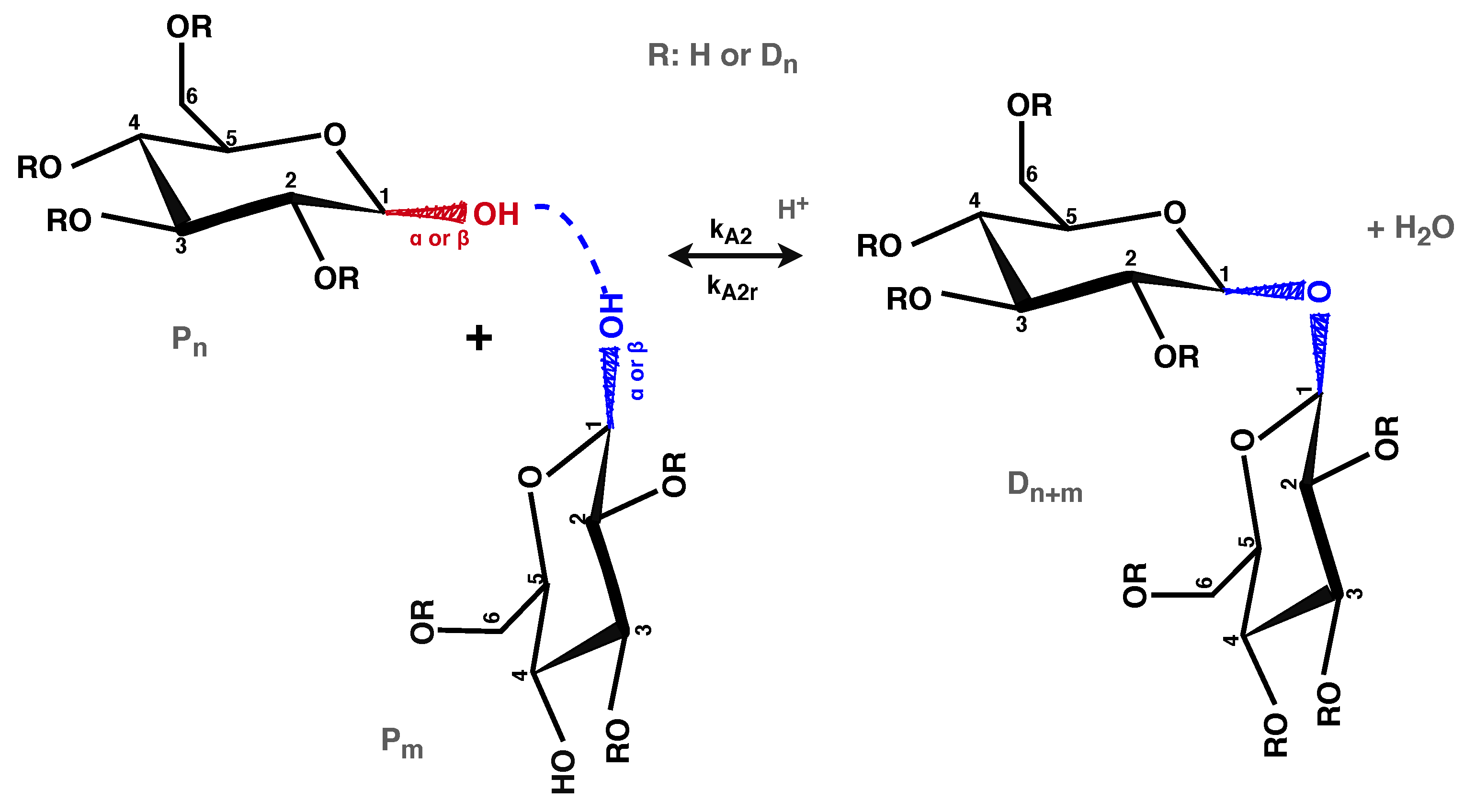
The chemical reactions of the postulated kinetic scheme have been grouped into three main categories. The first category includes the chemical reactions that lead to the formation of intermolecular bonds, via the addition of a hydroxyl group of a sugar molecule or polyol to the carbocation at the C1 carbon atom of a reducing saccharide (Equations (1)–(7)). These reactions are reversible by the respective hydrolysis reactions. To add flexibility to the model, the free hydroxyl groups of anhydrosugars have also been considered susceptible to participate in these reactions (Equations (6) and (7)). More precisely, the reactions between two reducing saccharides have been considered to result in the formation of another reducing saccharide, as shown in Equation (1), only in the case of the formation of a bond in positions 1-2, 1-3, 1-4 or 1-6. An example of such a reaction for the formation of a 1-6 bond is depicted in Scheme 1. If the glycosidic bond between two reducing saccharides is formed in position 1-1, then the resulting saccharide is a non-reducing one as it no longer possesses a free anomeric hydroxyl group, as shown in Equation (2) and in Scheme 2.
On the other hand, the formation of a glycosidic bond between a reducing and a non-reducing saccharide, will always result in the formation of a non-reducing saccharide, irrespective of the position of the bond (the formation of a 1-1 bond is not possible in this case). This is illustrated in Equations (3) and (4), as well as in Scheme 3.
Note that, a non-reducing saccharide can also be formed, besides the aforementioned mechanisms, by the reaction of a reducing saccharide with a polyol (Equation (5)) or with another anhydrosugar (Equations (6) and (7)). Accordingly, the second category of reactions contains the spontaneous formation of these anhydrosugars, via the creation of intramolecular linkages, as shown in Equations (8) and (9). In the present modeling work, it has been considered that these reactions may take place both on single glucose molecules (i.e., Equations (8) for n = 1 and (9)), as well as on the chain-end glucose units of higher-DP saccharides (i.e., Equation (8) for n 2 ). An example of Reaction (8) is illustrated in Scheme 4. Finally, the last category includes the degradation reactions that lead to the formation of Humins.
Attention should be paid to the fact that the form of reaction (4) reduces to that of reactions (5)–(7), for m = 0 and for X : P O , A G or H M F , respectively. However, the kinetic mechanisms described by these reactions is not the same. In fact, reaction (4) describes the formation/hydrolysis of the glycosidic bonds between the glucose units of the participating saccharides (i.e., between the units 1 to n of a saccharide of type D n X ), as shown in Scheme 3, while reactions (5)–(7) concern exclusively the bonds between the penultimate glucose unit and the end-group of type X, that are not covered by reaction (4) (i.e., the bond between the nth glucose unit and X, of a saccharide of type D n X ).
Note that, the above kinetic scheme contains only lumped reactions, without detailing the elementary mechanisms, as is the commonly adopted strategy in the relevant literature. Note also that, despite the multifunctional character of the glucose units that leads to the formation of branched saccharides, the fact that not all possible combinations of hydroxyl groups can lead to the formation of glycosidic bonds (i.e., since the participation of the carbocation at the C1 carbon atom of a reducing saccharide is required), as well as the significant extent of hydrolysis in the reaction medium, makes the formation of irreversible crosslinked networks unlikely.

2.2. Structural Characteristics of the Sugar Molecules

The development of the model equations describing the evolution of the concentration and the properties of the different sugar molecules necessitates the consideration of the individual structural characteristics of each species, such as their number of hydroxyl groups and bonds, with respect to their DP. In the present work, the hydroxyl groups of the saccharides are distinguished into two types, namely the anomeric and the susceptible hydroxyl groups. The first type refers to the hydroxyl groups that are attached to the anomeric carbon atom located at position 1 of reducing saccharides and are denoted in the model equations as O H 1 . The second type describes the rest of the hydroxyl groups that are susceptible to create a bond with an anomeric carbon, without considering eventual steric limitations. These are denoted as O H s . Note that, the number of anomeric and susceptible hydroxyl groups, found on a single individual sugar molecule, depends on the latter’s type, DP and end-unit. Accordingly, each sugar molecule possesses a number of O H s that is proportional to its DP and to its end-group, but may only posses one (or none) anomeric hydroxyl group, irrespective of its DP. For example, a saccharide ending in a polyol group is a non-reducing saccharide that contains only susceptible hydroxyl groups. Furthermore, the total number of these groups is higher than the respective number of susceptible hydroxyl groups of a reducing saccharide, of the same DP, due to the presence of the polyol group on the chain-end of the former. These differences must be reflected in the respective rate functions of the different types of sugar molecules. Table 1, shows the structural characteristics of the different types of saccharides, in terms of the total number of hydroxyl groups and bonds (per molecule) found on each type of molecule.
In Table 1, p denotes the number of hydroxyl groups of the free polyol units, P O .

2.3. Rate Functions

On the basis of the postulated kinetic scheme for the system (Equations (1)–(11)), it is possible to derive the rate functions describing the net rates of production of the different sugar molecules that are present in the reacting system. Concerning the macromolecular sugars, these expressions are defined in terms of the respective chain-length of each molecule (i.e., in terms of its number of glucose units). Accordingly, the rate function of the reducing sugar molecules of size n, P n takes the following form:
r P n = k A 1 [ P n ] · m = 1 [ O H s P m ] + [ O H s P n ] · m = 1 [ P m ] k A 1 r · [ B P n ] · [ H 2 O ] + 2 k A 1 r · [ H 2 O ] · m = n + 1 [ P m ] + k A 1 · m = 1 n 1 [ O H s P m ] · [ P n m ] 2 k A 2 · [ P n ] · m = 1 [ P m ] + k A 3 r · [ H 2 O ] · m = n + 1 ( [ D m ] + [ D m X ] ) + k A 2 r · [ H 2 O ] · m = n + 1 [ D m ] k A 3 · [ P n ] · m = 1 ( [ O H s D m ] + [ O H s D m X ] ) k D 1 · [ P n ] + k D 1 r · [ H 2 O ] · [ D n 1 A G ] k A 4 · [ O H s P O ] + k A 5 · [ O H s A G ] + k A 6 · [ O H s H M F ] · [ P n ] + k A 4 r · [ D n P O ] + k A 5 r · [ D n A G ] + k A 6 r · [ D n H M F ] · [ H 2 O ] + ( k D 1 r · [ H 2 O ] · [ A G ] ( k D 2 + k D 3 ) · [ P n ] ) · δ ( n 1 )
The rate, r P n , is expressed in units of molar concentration over time (i.e., mol L 1 min 1 ), while the molar concentrations of the different species (i.e., in mol L 1 ) are denoted with the use of brackets []. Finally, B P n designates the number of bonds of the reducing saccharides of DP equal to n and δ ( n 1 ) is the Kroenecker’s delta, given by:
δ ( n i ) = 1 for n = i 0 for n i
The rate functions for the rest of the polysaccharides can be defined accordingly, in terms of their respective DP. Besides the macromolecular species, the system contains also different types of monosaccharides, polyol molecules and water. The evolution of the quantities of these species is described by similar rate functions, always defined on the basis of the postulated kinetic scheme. Accordingly, the net rate of formation of free polyol molecules in the reacting mixture is described by the following expression:
Polyol molecules, P O
r P O = k A 4 · [ O H s P O ] · n = 1 P n + k A 4 r · [ H 2 O ] · [ D n P O ]
The analytical expressions of the rate functions of the rest of the macromolecular and non-macromolecular species are given in Appendix A (Equations (A1)–(A9)).

2.4. Reactor Design Equations

Once the rate functions of the species are defined, it is possible to derive the design equations for a batch reactor, in the form of a system of ordinary differential equations (ODEs):
1 V d V · [ M S n ] d t = r M S n ; n = 1 , 2 , . . .
1 V d V · [ S ] d t = r S
In the above expressions, [ M S n ] and [ S ] denote respectively the molar concentration of the different macromolecular and non-macromolecular species of interest, appearing in the established rate functions, n being the DP of the former. V is the volume of the reacting mixture, which also varies according to:
d V d t = K w · A · ( x W x W * ) d W
where d W denotes the molar density of water, K W is the water evaporation constant and A is the evaporation surface. x W and x W * denote the respective instantaneous and equilibrium molar fractions of water in the reactor. For the calculation of x W * , an activity coefficient thermodynamic model was employed, whose coefficients have been adjusted by the company ROQUETTE on the basis of the experimental data.

3. Model Developments

3.1. Method of Moments

The formulation of the rate functions in terms of the DP of the different molecules results in a system of coupled material balances that need to be solved simultaneously. Since the number of equations of the system is dictated by the maximum considered DP of each type of sugar molecule, one needs to presuppose its value and constrain the solution to this assumption. Several techniques have been proposed for the numerical solution of such systems, in view of calculating key properties of the produced polymers, such as the average molecular weights or the complete distributions. A relevant detailed discussion of such approaches can be found elsewhere [26,27]. Among them, one of the most commonly employed approaches to reduce the size of the system is the method of moments [28]. It is a widely-used technique, especially in the modeling studies of polymerization systems, that is based on the statistical representation of the average molecular properties of the macromolecular species in terms of the leading moments of their number-chain-length distribution. Accordingly, the moment of order k, for the reducing sugar molecules, P n , can be defined as:
λ k = n = 1 n k P n
The moments for the other types of sugar molecules can be defined accordingly. On the basis of the above definition of the moments, the rate functions of the different saccharides can be readily transformed to express the rate functions of their respective moments. All these expressions are presented in detail in Appendix A (Equations (A10)–(A20)). Accordingly, the reactor design equations, describing the evolution of the quantities of the different macromolecular species in a batch reactor (Equation (15)), are also transformed to describe the evolution of the respective leading moments of these species, thus significantly reducing the size of the system of ODEs:
1 V d V · [ M M S k ] d t = r M M S k ; k = 0 , 1 , 2
where [ M M S k ] denotes the moment of the macromolecular species, S, of order k. The implementation of the method of moments provides the advantage that certain moments can be directly related to specific magnitudes and properties of the system. As such, the zeroth moment of the reducing sugars, λ 0 , corresponds directly to the number of anomeric hydroxyl groups that are present, at any moment, in the reacting mixture. This provides a useful indication of the capacity of the system to continue reacting towards higher DP. Similarly, the total amount of glucose units, that are present on the different sugar molecules, can be calculated by Equation (20). Since this quantity remains constant throughout the process, it can also be used to validate the correct implementation of the moment rate functions of the model (i.e., by verifying its value throughout the duration of the simulation):
[ G ] = λ 1 + ϕ 0 + ω 0 + μ 1 + [ A G ] + [ H M F ]
where the moments λ k , ϕ k and ω k correspond respectively to the macromolecular species P n , D n A G and D n H M F (see Appendix A) and μ 1 is the 1st order moment of all the non-reducing sugar molecules (i.e., in general: μ k = ξ k + ψ k + ϕ k + ω k ).
The calculation of the average molecular weights of the sugars, at any given moment in the system, is straightforward from their respective moments, according to the following expressions:
M n = λ 1 + μ 1 λ 0 + μ 0 · ( M G M H 2 O ) ; M w = λ 2 + μ 2 λ 1 + μ 1 · ( M G M H 2 O )
in the above expressions, M G and M H 2 O denote the molecular weights of a glucose molecule and a water molecule, respectively. Note that the above calculation of the average molecular weights is only approximate as it does not take into account the type of end-unit of each molecule.
Despite its aforementioned advantages, the method of moments presents a significant drawback. As can be seen in the postulated moment rate functions of the macromolecular saccharides (Equations (A10)–(A14)), some terms of the expressions create a dependency of a moment of order k on a moment of order k + 1 (i.e., the so-called moment-closure problem). To overcome this problem and close the mass balances of the system, several closure techniques have been reported in the literature for different polymerization systems [29,30]. However, as these closure techniques depend on the form of the chain-length distribution of the produced macromolecular species, they are not directly transferable to different systems, as is the case of sugars. Indeed, the multimodal character of the chain-length distributions of the polysaccharides does not allow a direct implementation of the reported techniques. At the same time, other closure techniques that do not depend on the form of the chain-length distribution and take advantage of the quantitative difference between moments of different species, as is the technique proposed by [31], are also not applicable to this system, due to the absence of such quantitative difference between the sugar species.
To overcome this problem for this system, different solutions could be envisaged. The first one would be to couple the system of ODEs of the model (Equations (16), (17) and (19)) with Equation (20) in order to estimate, within each step of the integration, the values of the terms related to the closure problem. However, this approach is computationally complex and prone to numerical instabilities. A different approach would be to adopt simplifying assumptions that would allow the consideration of a simpler kinetic scheme, thus eliminating these terms from the model equations altogether.

3.2. The Kinetic Monte Carlo Algorithm

An alternative to the implementation of any deterministic approach, such as the method of moments, for the modeling of reactive systems, is to implement a stochastic modeling approach. Monte Carlo (MC) techniques provide this alternative via the use of random sampling (i.e., in terms of a pseudo-random number generator) and their fields of application include problems varying from numerical quadrature to statistical physics and finance [32,33,34,35]. In the modeling of polymerization reaction kinetics, two principal MC techniques have found the most widespread application, namely the Stochastic Simulation Algorithm (SSA) of [36] and the approach of [37], on the basis of primary polymer molecules. In general, MC is particularly suitable for the description of dynamically-evolving multi-body systems that are characterized by stochastic state transitions and a relative complexity in the definition of the constituting elements of the system. These characteristics are typical of batch polymerization systems where the formed polymer displays structural complexity, such as non-linearity, multi-functionality, etc. In this respect, the polycondensation of sugars presents an excellent system for such a stochastic modeling approach.
Following the original developments of the SSA of [36], the reactive system, that is considered spatially homogeneous, is represented by a finite sample of molecules of all the participating species. These are subsequently subject to a series of stochastically occurring interaction steps, according to a set of dynamically varying instantaneous probabilities. These interaction steps represent the different reactions of the system’s kinetic scheme, while their occurrence probabilities reflect their respective rates, depending on the kinetic constants and on the instantaneous molecular quantities of the different species in the simulation sample. The general expressions dictating the application of the SSA on polymerization systems, concerning the stochastic selection of the reaction event to be simulated in a given time step, as well as the calculation of the corresponding time-step duration, have been extensively presented in other studies [38,39] and, as such, are omitted from the present work. On the other hand, the details concerning the implementation of the MC algorithm to this specific system are presented in the following paragraphs.
The implementation of the MC formulation to the present system is based on the straightforward application of the above basic principles of the SSA. In this respect, a series of different species, indexes and properties are monitored throughout the temporal evolution of the reacting system. These species include the different types of reducing and non-reducing sugar molecules, as defined in the postulated kinetic scheme, water molecules and polyol molecules. All these constitute the reacting units of the simulated sample, whose quantity and properties are monitored by the developed kinetic MC algorithm, throughout the polymerization. More precisely, among the properties that are monitored, are the chain length of the different sugar molecules, in terms of their constituting number of glucose units, their exact number of glycosidic bonds, as well as their number of hydroxyl groups, both anomeric and susceptible ones.
The monitoring of the above quantities serves for the calculation of the instantaneous values of the reaction probabilities, as well as for the continuous tracking of the key properties of interest of the produced saccharides. Accordingly, at any given instant during the reaction, it is possible to infer detailed information about the molar mass of any molecule that is present in the system, via the tracking of their chain length and type (i.e., end-unit). It is also possible to follow the capacity of the system to continue creating new glycosidic bonds, via the evolution of the hydroxyl groups, as well as its hydrolysis rates, via the tracking of the formed bonds and the quantity of water molecules. The analytical expressions of the instantaneous rates of the different chemical reactions of the kinetic scheme, as transformed on the basis of the previously established rate functions (see Section 2.3), are presented in Table 2.
In the expressions appearing in Table 2, O H s S is the total number of susceptible hydroxyl groups of the molecules of type S, in the simulation sample, and B S represents the respective total glycosidic bonds between the glucose units of the molecules of type S. Finally, W denotes the number of water molecules in the sample. These quantities are calculated on the basis of the information that is tracked, in the MC algorithm, for every single molecule of the simulation sample, as well as on the basis of the instantaneous water evaporation rate (see Equation (17)).
A significant advantage of the MC formulation, over commonly employed deterministic approaches (i.e., such as the previously presented moments formulation), is that the different characteristics of the various species are tracked in detail, for every single saccharide, thus avoiding the necessity to use approximate expressions or simplifications to calculate the properties of interest. This becomes evident, for example, in the calculation of the average molecular weights that are directly inferred by their definition expressions:
M n = i = 1 N M M M M i N M M ; M w = i = 1 N M M M M i 2 i = 1 N M M M M i
where M M i is the exact molecular weight of molecule ‘i’, and N M M is the total number of molecules taken into account for the calculation of the corresponding property, including reducing and non-reducing saccharides with different chain-end groups. For example, the molecular weight of two polysaccharides, each composed of n glucose units, the first one being a reducing polysaccharide and the second one being a non-reducing polysaccharide ending in a polyol unit, will be respectively:
M M i P n = n · M G ( n 1 ) · M H 2 O M M i D n P O = n · ( M G M H 2 O ) + M P O
In the above expressions, M G , M H 2 O and M P O denote the molecular weights of a glucose molecule, a water molecule and a polyol molecule, respectively. Note that, contrary to radical polymerization systems, the calculation of the molar mass of the different species, present in this system, by a typical expression of the type: M M i = n · D n · M m u , would not be exact, due to the existence of different types of end-group and different amounts of hydroxyl groups on the sugar molecules as well as due to the relatively low degrees of polymerization of this system, in comparison to a classical radical polymerization system. Hence, any expression of the average molecular weights, based on such an approach (i.e., that is unavoidable in the case of the commonly employed deterministic modeling techniques), can only be approximate. This problem does not exist in the case of the MC formulation where the detailed chain length and structure of the participating molecules are available throughout the course of the reaction.
The kinetic MC algorithm also provides the ability to track the evolution of the complete molecular weight distribution (MWD) developments of the macromolecular species, in contrast to the moments formulation. For the reconstruction of the complete MWD by the MC algorithm, the molar mass domain of the different saccharides must initially be discretized in a number of discretization bins, β i . In the present work, the following discretization rule is adopted:
β i = M m i n · 2 ( i 1 ) / q ; i = 1 , . . , N e
where M m i n denotes the minimum considered value of the molar mass and q is a discretization parameter. The total number of discretization bins, N e , can be calculated as a function of the length of the considered molecular weight domain, [ M m i n , M m a x ] , and of the parameter, q, according to the expression:
N e = I n t 1 + q · ln ( M m a x / M m i n ) ln 2 + 1
where ‘ I n t ’ denotes the integer part of the corresponding value. In the present work, the considered molecular weight domain extended from M m i n = 100 g mol 1 to M m a x = 2 · 10 4 g mol 1 and the value of the parameter q was set to 3.2. Finally, another advantage of this approach is that there is no requirement for a closure technique.

3.3. Tracking the Structural Characteristics of the Sugar Molecules

Both the method of moments and the MC method rely on the calculation and tracking of the structural characteristics of the different saccharides, as presented previously in Section 2.2. This becomes evident by the form of the respective moment rate functions (Equations (A10)–(A14)) and instantaneous rates (Table 2) of the two methods. According to the description of these characteristics, per type of molecule, given previously in Table 1, it is possible to derive generic expressions for the calculation of the number of hydroxyl groups and glycosidic bonds for each saccharide within each modeling approach. Accordingly, although the number of anomeric hydroxyl groups is explicitly defined for every type of saccharide (i.e., equal to 1 only for the reducing saccharides and 0 for all the rest), the number of susceptible hydroxyl groups needs to be defined in terms of the DP of each type of sugar. In the present modeling work, this has been achieved by the use of the following expression:
O H s X n = a X · n + b X
where O H s X n denotes the number of susceptible hydroxyl groups per molecule of type X n , n being its respective DP, and a X and b X being its characteristic coefficients. The values of these coefficients are given in Table 3. Note that, the implementation of this generic expression provides flexibility to this modeling framework and facilitates its eventual implementation to similar systems containing other forms of saccharides (e.g., sucrose, fructose, etc.). However, it should be emphasized that these coefficients do not constitute additional tunable parameters of the model as their values are explicitly defined by the structures of the corresponding saccharides, without them being subject to any form of adjustment or tuning.
According to the above, the calculation of the total concentration of susceptible hydroxyl groups of the molecules of type X n , as encountered in the moment rate functions (Equations (A10)–(A14)), will be directly calculated by:
[ O H s X n ] = a X · n + b X · [ X n ]
In the same way, the total quantity of the same susceptible hydroxyl groups, required for the calculation of the MC instantaneous rates (Table 2), will be calculated as:
O H s X n = n = 1 a X · n + b X · X n
Note that, for the respective calculation for the non-macromolecular species, such as A G , P O and H M F , it suffices to set n = 0 in the above expressions.

3.4. Kinetic Rate Constants

The rate constants of the different reactions of the adopted kinetic scheme, representing the principal parameters of the proposed model, need typically to be determined on the basis of available experimental data. These 17 parameters in total (i.e., k A 1 - k A 6 , k A 1 r - k A 6 r , k D 1 - k D 4 and k D 1 r ) can be classified into two main categories, i.e., the parameters of the polycondensation reactions, leading to the formation of a bond with the parallel release of water, and those of the hydrolysis reactions, leading to the scission of the formed bonds. Within each of the above two categories, one could further distinguish the internal ring-closure reactions and the degradation reactions from the rest of the reactions that take place between two different saccharides. These categories have already been identified in the presentation of the postulated kinetic scheme, in Equations (1)–(11). This significantly reduces the considered lumped reaction events and their corresponding kinetic rate constants, provided that a global rate constant is considered for each category.
The determination of all 17 parameters would certainly add flexibility to the model and, eventually, a higher prediction accuracy since more degrees of freedom would be available for fitting the experimental data. On the other hand, the consideration of a reduced set of rate constants, on the basis of the aforementioned lumped reaction events (or categories), seems to be more realistic from a chemical viewpoint. For example, it would be natural to assume that the rate constants of the reactions (1) and (3) should not be significantly different, for the same type of bond. Note that, the consideration of individual formation and/or hydrolysis rates of the different types of bonds (i.e., 1-1, 1-2, 1-3, 1-4 1-6, in position α or β ), in terms of steric hindrance effects, would be absolutely relevant and supported by reported data [15,17,20,22]. However, this distinction is not possible in the proposed modeling framework, under the method of moments or the kinetic MC formulation, as the types of bonds are not monitored during the reactions. Such a consideration would only be possible within a topological MC modeling approach, which would provide the possibility to record and follow the structural characteristics of the saccharides in more detail, as has been shown in other polymerization systems [40].
In the present work, the assumption that the reduced set of five rate constants is sufficient to describe the evolution of the system has been adopted and tested on the basis of the available experimental data. Accordingly, the considered rate parameters have been reduced to: k A ( = k A i , i = 1 : 6 ) , k A r ( = k A r i , i = 1 : 6 ) , k D 1 , k D 1 r and k D 2 . Finally, considering the degradation reactions (10) and (11), their respective kinetic rate constants have been considered unidentifiable. This is due to the fact that the average molar mass of the degradation products (Humins) has been considered equal to that of HMF [25], as well to the fact that the available experimental data did not contain any information allowing us to quantify them individually.
The parametric identification procedure of the above five rate constants was carried out manually, given their low number and the stochastic nature of the MC algorithm, starting from reported values of similar reacting systems [22]. This procedure was repeated for each reaction temperature for which experimental data were available (i.e., at 160 °C, 170 °C, 180 °C and 190 °C). Finally, the values of the pre-exponential constants and of the activation energies of Arrhenius-type expressions were determined via linear regression. These values are reported in Table 4, along with the expression allowing the calculation of the water evaporation rate (Equation (17)).
Note that, all available experimental data were obtained using a constant concentration of the same acid catalyst (cf. Section 5). In this respect, it would be meaningless to include a term, in the kinetic rate expressions, accounting for the catalyst concentration, since the determination of its value would be without statistical significance. A comparison with the relevant literature [22], shows that the obtained parameter values are comparative to the reported ones. For example, the values of k D 1 , k D 2 and k A r are in the same order of magnitude with the respective reported values while the value of k A is about one order of magnitude lower. However, this comparison can only be used to provide a general idea of the positioning of the estimated values with respect to reported ones, since the kinetic scheme that is adopted in this work is not directly comparable with any other reported work. It should also be noted that, due to the absence of corroborating experimental observations of diffusion-controlled phenomena [41,42], both in this study and in the relevant literature, no such effects have been considered in the developed model. In any case, should the need appear to include such phenomena, this would be straightforward, considering the form of the developed model.

4. Experimental

A series of polymerization experiments was carried out by the company ROQUETTE, under different experimental conditions, and the generated data were used for the calibration and the validation of the developed mathematical model. These experiments were carried out in a vacuum-tight thermo-microbalance analyzer, NETZSCH TG 209 F1, under four different reaction temperatures in the range of 160 °C to 190 °C. The pressure during the reactions was kept constant at 2 · 10 4 Pa in order to control the humidity level of the reaction medium, thus favoring the polycondensation reactions over their hydrolysis counterparts. The initial medium composition, in all tested temperatures, was composed of 90.1 wt% of maltose disaccharide (1,4-O- α -d-glucopyranosyl-d-glucose), 9.0 wt% of the polyol maltitol (4-O- α -d-glucopyranosyl-d-glucitol) and 0.9 wt% of citric acid (2-hydroxypropane-1,2,3-tricarboxylic acid), which served as catalyst. The overall initial mass, for all the experiments, was approximately 0.05 g.
For each reaction temperature, several polymerization experiments were carried out with different duration in order to monitor the evolution of the conversion and molar mass indexes. In this respect, after the end of each polymerization, the reaction medium was analyzed by size exclusion chromatography (SEC), in a column equipped with a refractive index detector, while its calibration was carried out on the basis of pullulans and maltooligosaccharides of known molar mass. All the tested conditions, in terms of the reaction temperature and pressure, as well as in terms of the initial syrup composition, are completely relevant to the industrial production practice.

5. Model Results and Discussion

Due to the aforementioned limitations of the method of moments, mainly related to the moment closure problem, it was considered that the most fitted approach for the modeling of this system was that of the kinetic Monte Carlo algorithm, as described in Section 3.2. Accordingly, the model predictions presented in this section were generated solely via the implementation of this method. Following the experimental conditions (see Section 4), the initial sample of the MC simulations was composed of polyol molecules and disaccharides. A typical size of this sample, for the simulations presented here, was equivalent to 3 · 10 5 glucose units (i.e., distributed on the initially formed disaccharides) and 1.5 · 10 4 polyol molecules. This sample size, that was determined via the procedure described in [38], was sufficient for the generation of all the results presented in this section on the basis of a single simulation run. Finally, the program was developed in Matlab and the corresponding simulation time was of the order of 1 min, on a 3.6 GHz personal computer, without any code parallelization.
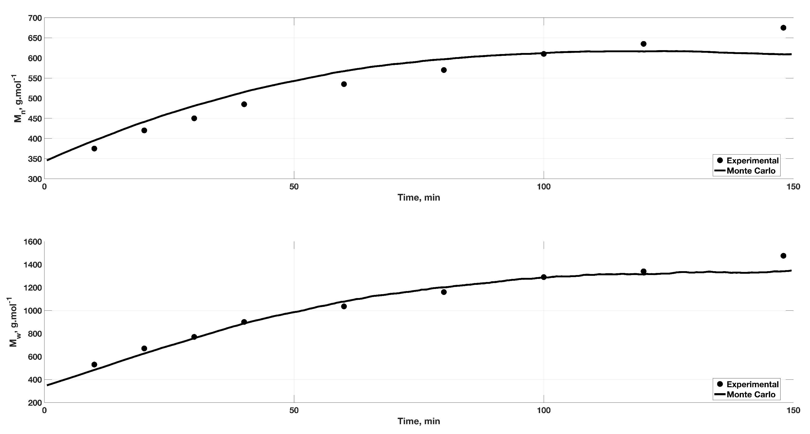
Figure 1 shows the comparison of the predictions of the model on the temporal evolution of the number- and weight-average molecular weights of the produced sugars with the respective experimental data, for the reactions carried out at 160 °C. The kinetic MC algorithm is capable of simulating the overall behavior of the mixture with very good accuracy, except the final experimental measurements that are slightly under-predicted. Note, that a single reduced set of values for the kinetic rate constants was used during the simulation of the system under the different reaction conditions (cf. Section 3.4).
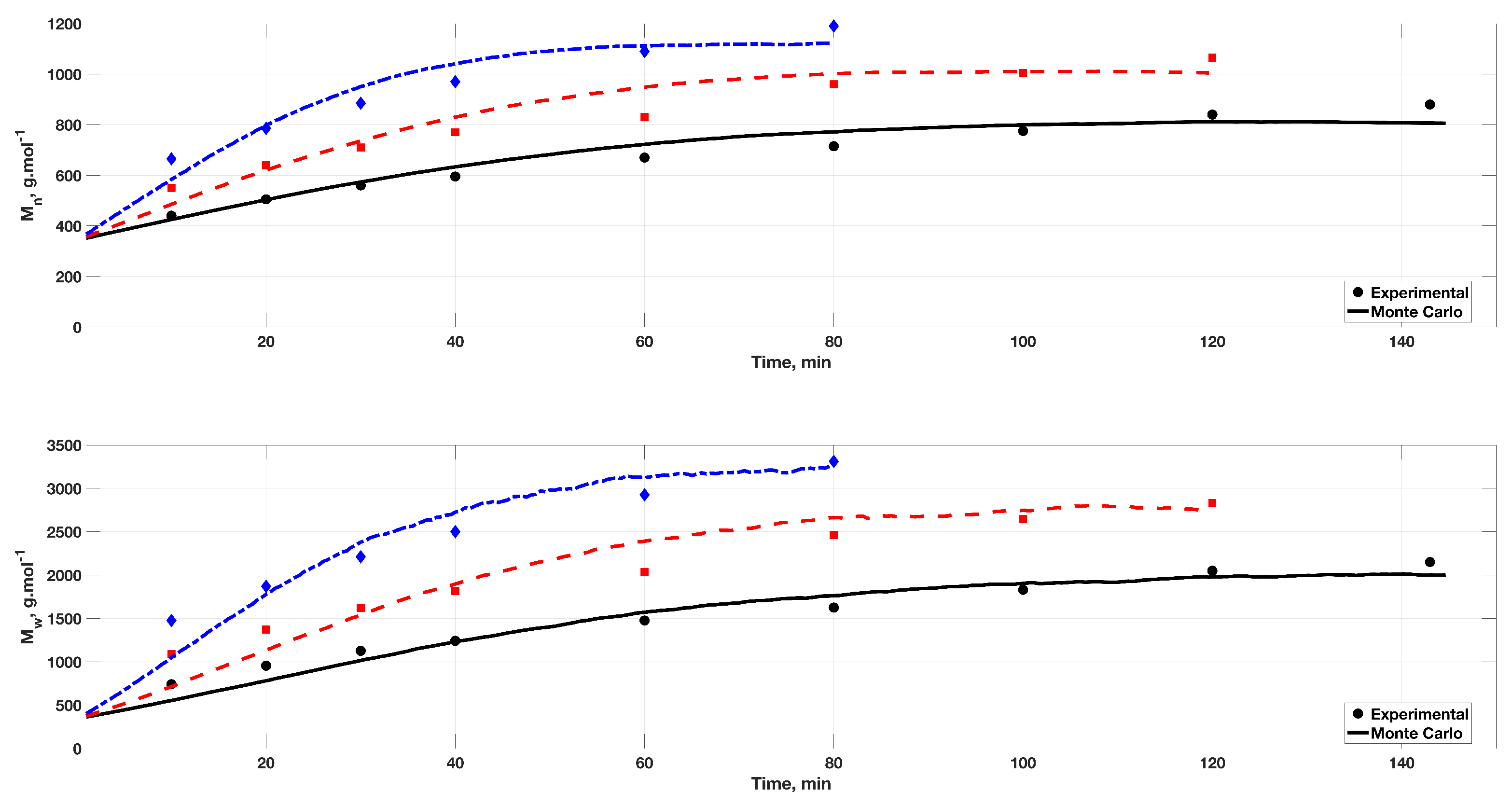
The same comparison for the rest of the tested reaction temperatures, namely for the experiments run at 170 °C, 180 °C and 190 °C, is shown in Figure 2. The observed increase of both average molecular weight indexes, with increasing temperature, was mainly due to the decrease of the rates of hydrolysis induced by the decreased humidity of the reacting mixture. The MC algorithm displays again a very good capacity in simulating the evolution of the system under different temperatures but presents the same under-prediction, with respect to the final experimental measurements. However, the fact that the duration of the polymerization reactions varied with the reaction temperature, reduces the probability of this fact being an indication of a subsequent increase of the experimental molecular weights that was not captured by the model predictions and strengthens the possibility that this deviation is simply part of the typically expected error between experimental data and modeling predictions (i.e., including experimental error and model uncertainties). Note that, the curves corresponding to the predictions of the model are not entirely smooth, which is characteristic of the results of the stochastic nature of the MC algorithm [39]. Note also that the number-average molecular weight of the produced polysaccharides, after 80 min of reaction at 190 °C, reached a value close to 1200 g mol 1 , which corresponds to an average DP of more than seven glucose units.
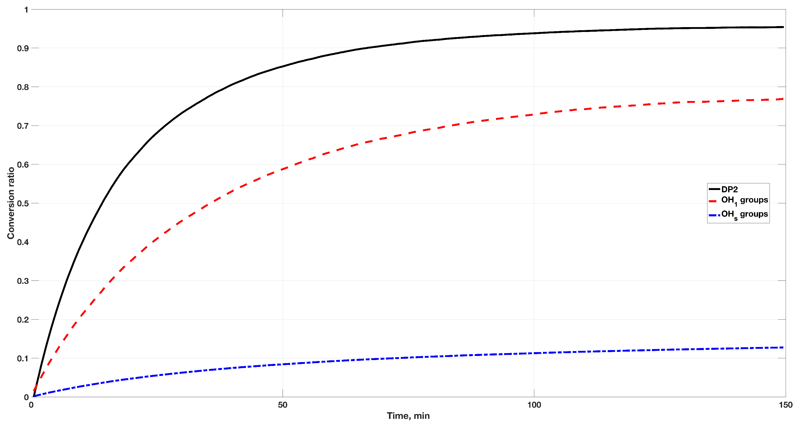
As discussed in Section 3.2, the proposed kinetic MC modeling framework allows for the monitoring of individual indexes and characteristics of interest of the sugars participating in the reaction. For example, Figure 3 shows the temporal evolution of the conversion of the disaccharide molecules, as well as that of the hydroxyl groups of all saccharides. More specifically, the conversion of the anomeric and susceptible hydroxyl groups are depicted separately in red and blue curves, respectively. This figure shows that the anomeric hydroxyl groups were consumed more rapidly than the susceptible ones, which can be explained by the fact that the vast majority of chemical reactions of the postulated kinetic scheme describes the consumption of equal amounts of susceptible and anomeric hydroxyl groups for the formation of a glycosidic intermolecular or intramolecular bond. Since the initial amount of susceptible hydroxyl groups was roughly four times higher than that of anomeric ones, it is normal that, in relative terms (i.e., in terms of a conversion ratio), the anomeric hydroxyl groups were consumed more rapidly along the polycondensation reactions. The only exceptions to the above rule are the reaction of creation of 1-1 glycosidic bonds (reaction (2)), which results to the consumption of two anomeric hydroxyl groups, and the reaction of spontaneous HMF creation (reaction (9)), which consumes three susceptible hydroxyl groups and only one anomeric group. However, their relevant extent was not significant enough to change the overall trend, observed in Figure 3. The same figure also shows that the disaccharides, which represented 90.1 wt% of the initial mixture, were rapidly consumed until an equilibrium was reached at around 95% of their conversion. Their consumption may lead to the formation of either monosaccharides or polysaccharides, via hydrolysis or polycondensation reactions, respectively.
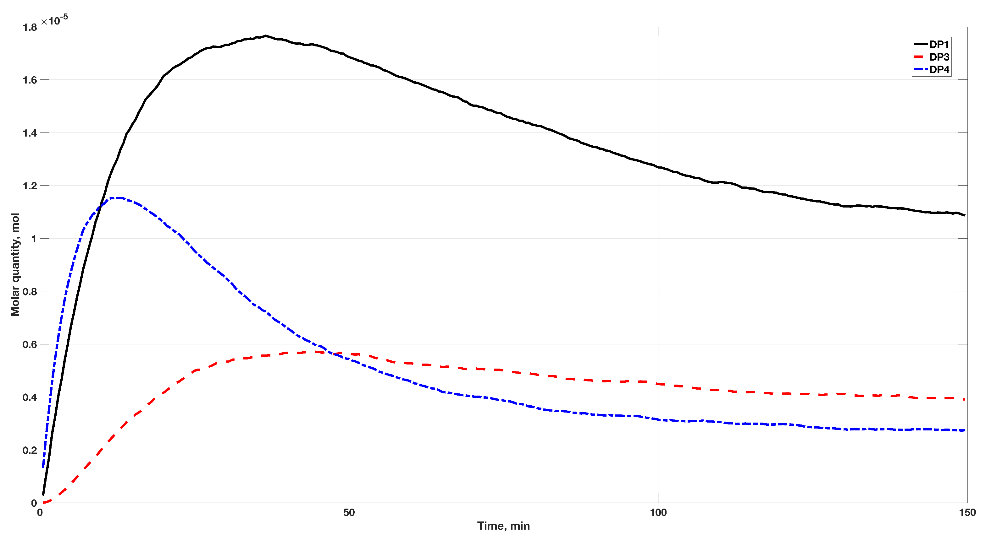
To further investigate these two potential routes, the evolution of the quantities of DP1, DP3 and DP4 sugars is depicted in Figure 4. From these curves, it becomes evident that, during the initial stages of the reaction, both the hydrolysis and the polycondensation of maltose proceeded in parallel. However, their respective rates were different. In fact, the formation of glucose, during these initial stages of the reaction at 160 °C, by the hydrolysis of maltose, prevailed that of the polycondensation of maltose to DP3 and DP4 sugars, which is also consistent with the rate constant values given in Table 4. However, as the quantity of formed glucose increased, so did their respective rate of polymerization, thus leading to a peak of the DP1 quantity curve, after approximately 45 min of reaction, and to a subsequent decrease during the rest of the polymerization. It is also seen that the quantity of formed sugars of DP4 increased with a higher rate than that of DP3 saccharides, probably due to the fact that, notably during the initial stages of the reaction, the molecules of maltose formed glycosidic bonds primarily among them (i.e., given their vast majority in the mixture), thus leading to the direct formation of DP4 sugars without forming the intermediate DP3 molecules. At the same time, the quantity of saccharides of DP3 displayed a delayed increase, with respect to that of the DP4 sugars, as the formation of a minimum quantity of glucose is a prerequisite for their synthesis via the reaction between DP1 and DP2 sugars.
After the initial peak and the subsequent stage of quantity decrease, the slopes of all curves reveal that the system gradually reached equilibrium at different rates and after a varying reaction duration for the different types of sugar molecules. The overall evolution of the curves is consistent with the respective evolution of the DP2 and O H 1 curves, presented in Figure 3. Accordingly, the fact that the rate of conversion of the anomeric hydroxyl groups was slower than that of the disaccharides, right from the start of the reaction, is probably due to the fact that, in parallel to their consumption, there was a significant rate of formation of O H 1 , via the hydrolysis of maltose.
The implementation of the MC method, in contrast to the method of moments, provides the additional advantage of tracking the analytical chain-length and structural characteristics of the sugar molecules participating in the reacting mixture. In this respect, it is possible to infer directly the MWD of the complete population of saccharides, at any given moment of the reaction. As example, Figure 5 depicts the MWD of the saccharides, at two different instances of the reaction at 160 °C, namely at the very beginning (i.e., after 10 min) and close to the end (i.e., after 1 h) of the reaction, for which experimental data were available. Both curves show clearly that the model possesses the capacity to follow the overall evolution of the MWD, mainly in terms of the relevant position of the different peaks. However, some peaks of the experimental spectra are over-predicted, especially at the very early stages of the reaction. This disagreement is more pronounced on the second peak of the spectrum, corresponding to the saccharides of DP2. At the same time, it is important to note that the MC method reconstructed the MWD on the basis of the molar mass of the different sugar molecules, which are, by the nature of the system, distinct discrete values. This is clearly visible in the form the MWD of the MC method that displays individual peaks, especially in the low-DP region of the figures where the discretization bins were narrow enough to contain individual saccharides (see Section 3.2). The peak values, calculated by the MC method, are marked by the filled blue circles on the graphs, while the connecting dashed-line curves correspond to a shape-preserving piecewise cubic interpolation between consecutive peaks. On the other hand, the experimental GPC curves display the typical continuous form that may also be subject to the commonly encountered resolution artifacts [43,44]. In any case, the overall areas covered by both experimental and MC spectra were consistent with each other.
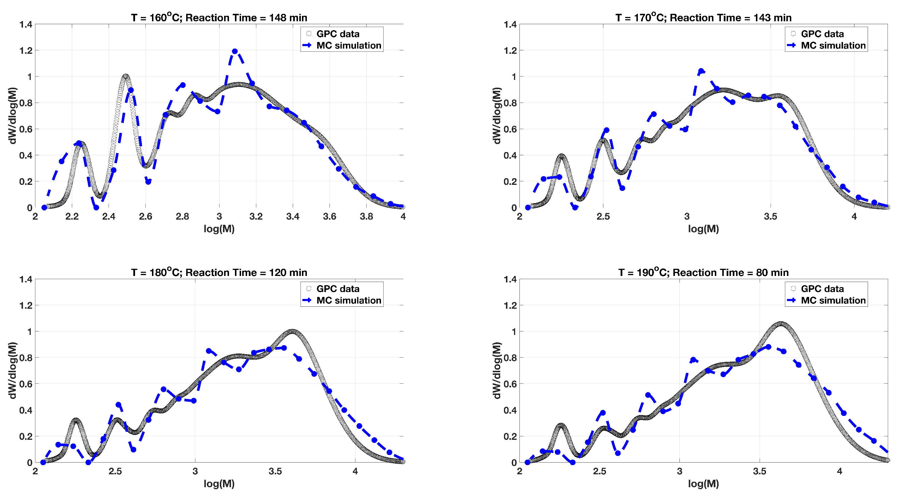
Finally, Figure 6 shows the comparison between the model predictions and the GPC experimental data of the MWD of the sugars obtained at the end of the reaction, at all four reaction temperatures. It is seen that, in all four cases, the peaks of the distributions corresponding to the low-DP sugars are significantly decreased, with respect to the beginning of the reaction, in parallel to the respective increase of the peaks at the higher-DP region. At the same time, these peaks are less distinct from one another and present a rather continuous multimodal character. This is mainly attributed to the fact that, as the value of the molar mass increases, the relative distance between the adjacent peaks of individual polysaccharides decreases, an effect that is more pronounced by the logarithmic scale of the horizontal axis. In terms of the MC predicted spectra, this effect is also reflected in the discretization rule of the molar mass domain (see Section 3.2). At the same time, the observed increase in the surface occupied by the higher-DP saccharides, with the reaction temperature, is also consistent with the effect observed in Figure 2.
Note that, the peaks observed mainly at temperatures above 170 °C, which are positioned at a value of l o g ( M ) around 3.6–3.8, correspond to polysaccharides of a DP in the range of 30–40 glucose units. In fact, at this temperature, although the vast majority of the polysaccharides (i.e., around 87% according to the MC model) displayed a DP < 10 glucose units, which is consistent with the evolution of the average molecular weights shown in Figure 2, there existed also a significant amount of polysaccharides with much higher DP, reaching at values even above 40 glucose units. These polysaccharides would be impossible to simulate via a modeling approach similar to those presented in the introduction of this work, which further supports and demonstrates the interest and the predictive capacity of the proposed modeling framework.

6. Conclusions

In the present work, a novel kinetic modeling framework was proposed for the system of polycondensation of sugars, in the presence of polyols and under strict control of the humidity of the mixture, in order to limit the hydrolysis reactions. The developed model was based on an extended and generalized kinetic scheme, which was established following a classical polymerization paradigm in order to allow for the consideration of the synthesis of polysaccharides of high degrees of polymerization. Accordingly, the different species were identified in terms of the number of their constituting glucose units, as well as in terms of other structural characteristics, such as their number of hydroxyl groups, either in anomeric position or any other position, and the existence of intramolecular bonds. For the formulation of the mathematical model equations, two different approaches were implemented, namely a deterministic one in terms of the method of moments and a stochastic kinetic Monte Carlo approach.
Through the derivation of the equations of the method of moments, it became evident that it does not consist of a viable modeling approach for this system, mainly due to its limitation with respect to the well-known moment closure problem, that appears in several terms, as well as due to its incapacity to predict the complete molecular weight distribution developments. However, in a more general consideration, the benefits of the method in terms of the direct relation of several properties and indexes of interest of the system with different moments were clearly presented. Via the present work, the implementation of this technique to several terms appearing in the rate functions of the polysaccharides, that are not commonly encountered in classical radical polymerization systems, was also demonstrated.
The predictions of the kinetic MC algorithm were compared against a series of experimental data, generated at four different reaction temperatures in the range of 160 °C to 190 °C. These comparisons demonstrated the capacity of the proposed model to predict, with very good accuracy, the evolution of the average molecular weights and the complete molecular weight distributions of the produced saccharides, even though a reduced set of only five kinetic rate constants was adopted. In addition to the comparisons with the experimental data, the model was employed to generate the evolution of several indexes of the polymerization, in an attempt to better illustrate the course of the reactions and the dominant reaction routes along the duration of the experiments.

Author Contributions

Conceptualization, all; methodology and model developments, D.M.; experimental analyses and data acquisition, B.B.; writing—original draft preparation, D.M.; writing—review and editing, all; funding acquisition, B.B. All authors have read and agreed to the published version of the manuscript.

Funding

This research was funded by ROQUETTE.

Institutional Review Board Statement

Not applicable.

Informed Consent Statement

Not applicable.

Data Availability Statement

Restrictions apply to the availability of these data. Data was obtained from ROQUETTE and are available from the authors with the permission of ROQUETTE.

Conflicts of Interest

The authors declare no conflict of interest.

Abbreviations

The following abbreviations are used in this manuscript:
DPDegree of Polymerization
GPCGel-Permeation Chromatography
MCMonte Carlo
MWDMolecular Weight Distribution

Appendix A. Model Equations

Appendix A.1. Rate functions of the Macromolecular Species

The net formation rates of all the macromolecular species that participate in the different chemical reactions can be established, on the basis of the postulated general kinetic scheme (Equations (1)–(11)), as follows:
  • Non-Reducing sugar molecules of size n, D n
    r D n = + k A 2 m = 1 n 1 [ P m ] · [ P n m ] k A 2 r · [ H 2 O ] · [ D n ] k A 3 · [ O H s D n ] · m = 1 [ P m ] + k A 3 m = 1 n 1 [ O H s D m ] · [ P n m ] k A 3 r · [ B D n ] m = n + 1 [ D m ] · [ H 2 O ]
  • Non-Reducing sugar molecules of size n, containing a polyol unit, D n P O
    r D n P O = + k A 4 · [ O H s P O ] · [ P n ] k A 4 r · [ H 2 O ] · [ D n P O ] + k A 3 · m = 1 n 1 [ O H s D m P O ] · [ P n m ] [ O H s D n P O ] · m = 1 [ P m ] + k A 3 r · [ H 2 O ] · m = n + 1 [ D m P O ] [ B D n P O ]
  • Non-Reducing sugar molecules of size n, containing a 1-6-anhydrosugar D n A G
    r D n A G = + k A 5 · [ O H s A G ] · [ P n ] k A 5 r · [ H 2 O ] · [ D n A G ] + k D 1 · [ P n + 1 ] k D 1 r · [ H 2 O ] · [ D n A G ] + k A 3 · m = 1 n 1 [ O H s D m A G ] · [ P n m ] [ O H s D n A G ] · m = 1 [ P m ] + k A 3 r · [ H 2 O ] · m = n + 1 [ D m A G ] [ B D n A G ]
  • Non-Reducing sugar molecules of size n, containing an HMF molecule D n H M F
    r D n H M F = + k A 6 · [ O H s H M F ] · [ P n ] k A 6 r · [ H 2 O ] · [ D n H M F ] + k A 3 · m = 1 n 1 [ O H s D m H M F ] · [ P n m ] [ O H s D n H M F ] · m = 1 [ P m ] + k A 3 r · [ H 2 O ] · m = n + 1 [ D m H M F ] [ B D n H M F ]
Finally, the rate function corresponding to the glucose molecules, P 1 , that appear in some of the above expressions, can be directly obtained by the respective rate function of the reducing sugar molecules (Equation (12)):
r P 1 = r P n · δ ( n 1 )

Appendix A.2. Rate Functions of the Non-Macromolecular Species

The net formation rates of the non-macromolecular species are established similarly, on the basis of the postulated kinetic scheme (Equations (1)–(11)):
1-6-anhydrosugar molecules, A G
r A G = ( 3 · k A 5 · n = 1 P n + k D 1 r · [ H 2 O ] ) · [ A G ] + k D 1 · [ P 1 ] + k A 5 r · [ H 2 O ] · n = 1 D n A G
HMF molecules, H M F
r H M F = ( k A 6 · n = 1 P n + k D 4 ) · [ H M F ] + k D 2 · [ P 1 ] + k A 6 r · [ H 2 O ] · n = 1 D n H M F
Humins, H
r H = k D 3 · n = 1 P n + k D 4 · [ H M F ]
Water molecules, H 2 O
r H 2 O = k A 1 · n = 1 P n · m = 1 [ O H s P m ] k A 1 r · [ H 2 O ] · n = 1 [ B P n ] + k A 2 · [ O H 1 P ] 2 + k A 3 · n = 1 P n · m = 1 [ O H s D m ] + [ O H s D m X ] k A 2 r · [ H 2 O ] · n = 1 [ D n ] k A 3 r · [ H 2 O ] · n = 1 [ B D n ] + [ B D n X ] + ( k A 4 · [ O H s P O ] + k A 5 · [ O H s A G ] + k A 6 · [ O H s H M F ] ) · n = 1 P n ( k A 4 r · n = 1 [ D n P O ] + k A 5 r · n = 1 [ D n A G ] + k A 6 r · n = 1 [ D n H M F ] ) · [ H 2 O ] + 3 · ( k D 2 + k D 3 ) · [ P 1 ] + k D 1 · n = 1 [ P n ] k D 1 r · [ H 2 O ] · n = 1 [ D n A G ] + [ A G ]

Appendix A.3. Moment Rate Functions

In accordance to the definition given in Equation (18), the moments λ k , ψ k , ξ k , ϕ k and ω k have been defined for the macromolecular species P n , D n P O , D n , D n A G and D n H M F , respectively. Next, on the basis of the previously defined rate functions (Equations (A1)–(A4)), the following rate functions can be established for the leading moments of the number-chain-length distributions of the above macromolecular species:
r λ k = k A 1 λ k · ( a P · λ 1 + b P · λ 0 ) + λ 0 · ( a P · λ k + 1 + b P · λ k ) + k A 1 r · [ H 2 O ] ( λ k + 1 λ k ) + 2 · m = 0 k k m B m k m + 1 · ( λ k m + 1 λ 0 ) + k A 1 · a P · m = 0 k k m λ m + 1 · λ k m + b P · m = 0 k · k m λ m · λ k m k A 3 · λ k · ( a D · ξ 1 + a D A G · ϕ 1 + a D P O · ψ 1 + a D H M F · ω 1 + b D · ξ 0 + b D A G · ϕ 0 + b D P O · ψ 0 + b D H M F · ω 0 ) 2 · k A 2 · λ k · λ 0 + k A 3 r · [ H 2 O ] · m = 0 k k m B m k m + 1 · ( μ k m + 1 μ 0 ) + k A 2 r · [ H 2 O ] · m = 0 k k m B m k m + 1 · ξ k m ( k A 4 · p · [ P O ] + k A 5 · 3 · [ A G ] + k A 6 · [ H M F ] ) · λ k + ( k A 4 r · ψ k + k A 5 r · ϕ k + k A 6 r · ω k ) · [ H 2 O ] ( k D 2 + k D 3 ) · [ P 1 ] k D 1 · λ k + k D 1 r · [ H 2 O ] · i = 0 k k i ϕ i + k D 1 r · [ H 2 O ] · [ D A G ]
  • Moments of the non-reducing sugar molecules of size n, ξ k
    r ξ k = + k A 2 m = 0 k k m λ k m · λ m k A 2 r · [ H 2 O ] · ξ k + k A 3 a D · m = 0 k k m ξ m + 1 · λ k m + b D · k m ξ m · λ k m k A 3 · λ 0 · ( a D · ξ k + 1 + b D · ξ k ) k A 3 r · [ H 2 O ] · ( ξ k + 1 ξ k ) + k A 3 r · [ H 2 O ] · m = 0 k k m B m k m + 1 · ( ξ k m + 1 ξ 0 )
  • Moments of the non-reducing sugar molecules of size n, containing a polyol unit, ψ k
    r ψ k = + k A 4 · p · [ P O ] · λ k k A 4 r · [ H 2 O ] · ψ k + k A 3 · a D P O · m = 0 k k m ψ m + 1 · λ k m + b D P O · k m ψ m · λ k m k A 3 · λ 0 · ( a D P O · ψ k + 1 + b D P O · ψ k ) + k A 3 r · [ H 2 O ] · m = 0 k k m B m k m + 1 · ( ψ k m + 1 ψ 0 ) ( ψ k + 1 ψ k )
  • Moments of the non-reducing sugar molecules of size n, containing a 1-6-anhydrosugar, ϕ k
    r ϕ k = + k A 5 · 3 · [ A G ] · λ k k A 5 r · [ H 2 O ] · ϕ k + k D 1 · i = 0 k k i · ( 1 ) k i · ( λ i [ P 1 ] ) k D 1 r · [ H 2 O ] · ϕ k + k A 3 · a D A G · m = 0 k k m ϕ m + 1 · λ k m + b D A G · m = 0 k k m ϕ m · λ k m k A 3 · λ 0 · ( a D A G · ϕ k + 1 + b D A G · ϕ k ) + k A 3 r · [ H 2 O ] · m = 0 k k m B m k m + 1 · ( ϕ k m + 1 ϕ 0 ) ( ϕ k + 1 ϕ k )
  • Moments of the non-reducing sugar molecules of size n, containing an HMF molecule, ω k
    r ω k = + k A 6 · [ H M F ] · λ k k A 6 r · [ H 2 O ] · ω k + k A 3 · a D H M F · m = 0 k k m ω m + 1 · λ k m + b D H M F · m = 0 k k m ω m · λ k m k A 3 · λ 0 · ( a D H M F · ω k + 1 + b D H M F · ω k ) + k A 3 r · [ H 2 O ] · m = 0 k k m B m k m + 1 · ( ω k m + 1 ω 0 ) ( ω k + 1 ω k )
In the above expressions, the Bernoulli numbers are defined as:
B j = 1 , 1 2 , 1 6 , 0 , . . . ; j = 0 , 1 , 2 , 3 . . .
According to the definition of the moments of the different species, the rate functions of the non-macromolecular species (Equations (A6)–(A9)) can be readily transformed, to eliminate the infinite summation terms.
Polyol molecules, P O
r P O = k A 4 · p · [ P O ] · λ 0 + k A 4 r · [ H 2 O ] · ψ 0
1-6-anhydrosugar molecules, A G
r A G = ( 3 · k A 5 · λ 0 + k D 1 r · [ H 2 O ] ) · [ A G ] + k D 1 · [ P 1 ] + k A 5 r · [ H 2 O ] · ϕ 0
HMF molecules, H M F
r H M F = ( k A 6 · λ 0 + k D 4 ) · [ H M F ] + k D 2 · [ P 1 ] + k A 6 r · [ H 2 O ] · ω 0
Humins, H
r H = k D 3 · λ 0 + k D 4 · [ H M F ]
Water molecules, H 2 O
r H 2 O = k A 1 · λ 0 · 3 · λ 1 + λ 0 ) k A 1 r · [ H 2 O ] λ 1 λ 0 ) + k A 3 · λ 0 · ( a D · ξ 1 + a D A G · ϕ 1 + a D P O · ψ 1 + a D H M F · ω 1 + b D · ξ 0 + b D A G · ϕ 0 + b D P O · ψ 0 + b D H M F · ω 0 ) + k A 2 · λ 0 2 k A 2 r · [ H 2 O ] · ξ 0 k A 3 r · [ H 2 O ] · ( μ 1 μ 0 ) + ( k A 4 · p · [ P O ] + k A 5 · 3 · [ A G ] + k A 6 · [ H M F ] ) · λ 0 ( k A 4 r · ψ 0 + k A 5 r · ϕ 0 + k A 6 r · ω 0 ) · [ H 2 O ] + 3 · ( k D 2 + k D 3 ) · [ P 1 ] + k D 1 · λ 0 k D 1 r · [ H 2 O ] · ϕ 0 + [ A G ] )

References

  1. Qian, X. Mechanisms and energetics for acid catalyzed β-d-glucose conversion to 5-hydroxymethylfurfurl. J. Phys. Chem. A 2011, 115, 11740–11748. [Google Scholar] [CrossRef] [PubMed]
  2. Hu, X.; Lievens, C.; Li, C.Z. Acid-catalyzed conversion of xylose in methanol-rich medium as part of biorefinery. ChemSusChem 2012, 5, 1427–1434. [Google Scholar] [CrossRef] [PubMed]
  3. Alonso, D.M.; Wettstein, S.G.; Dumesic, J.A. Bimetallic catalysts for upgrading of biomass to fuels and chemicals. Chem. Soc. Rev. 2012, 41, 8075–8098. [Google Scholar] [CrossRef] [PubMed]
  4. Yang, G.; Pidko, E.A.; Hensen, E.J. Mechanism of Bronsted acid-catalyzed conversion of carbohydrates. J. Catal. 2012, 295, 122–132. [Google Scholar] [CrossRef]
  5. Caes, B.R.; Teixeira, R.E.; Knapp, K.G.; Raines, R.T. Biomass to Furanics: Renewable Routes to Chemicals and Fuels. ACS Sustain. Chem. Eng. 2015, 3, 2591–2605. [Google Scholar] [CrossRef]
  6. Liu, L.; Li, Z.; Hou, W.; Shen, H. Direct conversion of lignocellulose to levulinic acid catalyzed by ionic liquid. Carbohydr. Polym. 2018, 181, 778–784. [Google Scholar] [CrossRef] [PubMed]
  7. Caratzoulas, S.; Davis, M.E.; Gorte, R.J.; Gounder, R.; Lobo, R.F.; Nikolakis, V.; Sandler, S.I.; Snyder, M.A.; Tsapatsis, M.; Vlachos, D.G. Challenges of and Insights into Acid-Catalyzed Transformations of Sugars. J. Phys. Chem. C 2014, 118, 22815–22833. [Google Scholar] [CrossRef] [Green Version]
  8. SriBala, G.; Vinu, R. Unified kinetic model for cellulose deconstruction via acid hydrolysis. Ind. Eng. Chem. Res. 2014, 53, 8714–8725. [Google Scholar] [CrossRef]
  9. Pascu, E.; Mora, P.T. Polycindensation of D-Glucose and other simple sugars in presence of acids. J. Am. Chem. Soc. 1950, 72, 1045. [Google Scholar] [CrossRef]
  10. Mora, P.T.; Wood, J.W. Synthetic Polysaccharides. I. Polycondensation of Glucose. J. Polym. Sci. 1958, 80, 685–692. [Google Scholar]
  11. Durand, H.W.; Dull, M.F.; Tipson, R.S. Polymerization of α-d-Glucose in the Solid State, in the Presence of Metaboric Acid. J. Am. Chem. Soc. 1958, 80, 3691–3697. [Google Scholar] [CrossRef]
  12. Rennhard, H. Polysaccharides and Their Preparation. U.S. Patent No.3.766.165, 25 May 1972. [Google Scholar]
  13. Pfizer Inc. Saccharide Polycondensation. GB Patent GB1422294A, 5 April 1974. [Google Scholar]
  14. Hu, X.; Kadarwati, S.; Wang, S.; Song, Y.; Hasan, M.D.; Li, C.Z. Biomass-derived sugars and furans: Which polymerize more during their hydrolysis? Fuel Process. Technol. 2015, 137, 212–219. [Google Scholar] [CrossRef]
  15. Long, Y.; Yu, Y.; Song, B.; Wu, H. Polymerization of glucose during acid-catalyzed pyrolysis at low temperatures. Fuel 2018, 230, 83–88. [Google Scholar] [CrossRef]
  16. Xu, Q.; Hu, X.; Shao, Y.; Sun, K.; Jia, P.; Zhang, L.; Liu, Q.; Wang, Y.; Hu, S.; Xiang, J. Structural differences of the soluble oligomers and insoluble polymers from acid-catalyzed conversion of sugars with varied structures. Carbohydr. Polym. 2019, 216, 167–179. [Google Scholar] [CrossRef]
  17. Long, Y.; Yu, Y.; Wu, H. Mechanistic insights into the primary reactions during acid-catalysed pyrolysis of levoglucosan at 80–140 °C. Fuel 2020, 268. [Google Scholar] [CrossRef]
  18. Saeman, J.F. Kinetics of Wood Saccharification-Hydrolysis of Cellulose and Decomposition of Sugars in Dilute Acid at High Temperature. Ind. Eng. Chem. 1945, 37, 43–52. [Google Scholar] [CrossRef]
  19. XIang, Q.; Kim, J.S.; Lee, Y.Y. A comprehensive Kinetic Model for Dilute-Acid Hydrolysis of Cellulose. Appl. Biochem. Biotechnol. 2003, 105–108, 337–352. [Google Scholar] [CrossRef]
  20. Girisuta, B.; Janssen, L.P.; Heeres, H.J. Green chemicals: A kinetic study on the conversion of glucose to levulinic acid. Chem. Eng. Res. Des. 2006, 84, 339–349. [Google Scholar] [CrossRef]
  21. Jing, Q.; Lü, X. Kinetics of Non-catalyzed Decomposition of Glucose in High-temperature Liquid Water. Chin. J. Chem. Eng. 2008, 16, 890–894. [Google Scholar] [CrossRef]
  22. Pilath, H.M.; Nimlos, M.R.; Mittal, A.; Himmel, M.E.; Johnson, D.K. Glucose reversion reaction kinetics. J. Agric. Food Chem. 2010, 58, 6131–6140. [Google Scholar] [CrossRef]
  23. Kupiainen, L.; Ahola, J.; Tanskanen, J. Kinetics of glucose decomposition in formic acid. Chem. Eng. Res. Des. 2011, 89, 2706–2713. [Google Scholar] [CrossRef]
  24. Tan-Soetedjo, J.N.; Van De Bovenkamp, H.H.; Abdilla, R.M.; Rasrendra, C.B.; Van Ginkel, J.; Heeres, H.J. Experimental and Kinetic Modeling Studies on the Conversion of Sucrose to Levulinic Acid and 5-Hydroxymethylfurfural Using Sulfuric Acid in Water. Ind. Eng. Chem. Res. 2017, 56, 13228–13239. [Google Scholar] [CrossRef]
  25. Sumerskii, I.V.; Krutov, S.M.; Zarubin, M.Y. Humin-Like substances formed under the conditions of industrial hydrolysis of wood. Rus. J. Appl. Chem. 2010, 83, 320–327. [Google Scholar] [CrossRef]
  26. Verros, G.D. Calculation of molecular weight distribution in non-linear free radical copolymerization. Polymer 2003, 44, 7021–7032. [Google Scholar] [CrossRef]
  27. Kiparissides, C. Challenges in particulate polymerization reactor modeling and optimization: A population balance perspective. J. Process Control 2006, 16. [Google Scholar] [CrossRef]
  28. Konstadinidis, K.; Achilias, D.S.; Kiparissides, C. Development of a unified mathematical framework for modelling molecular and structural changes in free-radical homopolymerization reactions. Polymer 1992, 33, 5019–5031. [Google Scholar] [CrossRef]
  29. Hulburt, H.; Katz, S. Some problems in particle technology. Chem. Eng. Sci. 1964, 19, 555–574. [Google Scholar] [CrossRef]
  30. Zabisky, R.C.; Chan, W.M.; Gloor, P.E.; Hamielec, A.E. A kinetic model for olefin polymerization in high-pressure tubular reactors: A review and update. Polymer 1992, 33, 2243–2262. [Google Scholar] [CrossRef]
  31. Lee, K.H.; Marano, J.P. Free-Radical Polymerization: Sensitivity of Conversion and Molecular Weights to Reactor Conditions. ACS Symp. Ser. Polym. React Process. 1979, 221–251. [Google Scholar] [CrossRef]
  32. Lim, C.; Nebus, J. Vorticity, Statistical Mechanics, and Monte Carlo Simulation; Springer Science & Business Media: New York, NY, USA, 2007. [Google Scholar]
  33. Dagpunar, J.S. Simulation and Monte Carlo: With Applications in Finance and MCMC; John Wiley & Sons: Hoboken, NJ, USA, 2007. [Google Scholar]
  34. Liu, J.S. Monte Carlo Strategies in Scientific Computing; Springer Science & Business Media: New York, NY, USA, 2008. [Google Scholar]
  35. Rubinstein, R.Y.; Kroese, D.P. Simulation and the Monte Carlo Method; John Wiley & Sons: Hoboken, NJ, USA, 2016; Volume 10. [Google Scholar]
  36. Gillespie, D.T. A general method for numerically simulating the stochastic time evolution of coupled chemical reactions. J. Comput. Phys. 1976, 22, 403–434. [Google Scholar] [CrossRef]
  37. Tobita, H. Molecular weight distribution in free radical polymerization with long-chain branching. J. Polym. Sci. Part B Polym. Phys. 1993, 31, 1363–1371. [Google Scholar] [CrossRef]
  38. Meimaroglou, D.; Krallis, A.; Saliakas, V.; Kiparissides, C. Prediction of the bivariate molecular weight-Long chain branching distribution in highly branched polymerization systems using Monte Carlo and sectional grid methods. Macromolecules 2007, 40, 2224–2234. [Google Scholar] [CrossRef]
  39. Meimaroglou, D.; Kiparissides, C. Review of Monte Carlo Methods for the Prediction of Distributed Molecular and Morphological Polymer Properties. Ind. Eng. Chem. Res. 2014, 53, 8963–8979. [Google Scholar] [CrossRef]
  40. Meimaroglou, D.; Kiparissides, C. A novel stochastic approach for the prediction of the exact topological characteristics and rheological properties of highly-branched polymer chains. Macromolecules 2010, 43, 5820–5832. [Google Scholar] [CrossRef]
  41. Keramopoulos, A.; Kiparissides, C. Development of a comprehensive model for diffusion-controlled free-radical copolymerization reactions. Macromolecules 2002, 35. [Google Scholar] [CrossRef]
  42. Achilias, D.S. A review of modeling of diffusion controlled polymerization reactions. Macromol. Theory Simul. 2007, 16. [Google Scholar] [CrossRef]
  43. Duerksen, J.H.; Hamielec, A.E. Molecular Weight Distribution. Part III. Gel Permeation Chromatography, Methods of Correcting for Imperfect Resolution. J. Polym. Sci. Part C Polym. Symp. 1968, 21, 83–103. [Google Scholar] [CrossRef]
  44. Duerksen, J.H.; Hamielec, A.E. Polymer reactors and molecular weight distribution. Part VII. Further development of gel permeation chromatography. J. Polym. Sci. Part C Polym. Symp. 1968, 12, 2225–2255. [Google Scholar] [CrossRef]
Scheme 1. Schematic representation of Reaction (1). The anomeric hydroxyl groups are marked in red and the formed linkages in blue.
Processes 09 00745 sch001
Scheme 2. Schematic representation of Reaction (2). The anomeric hydroxyl groups are marked in red and the formed linkages in blue.
Processes 09 00745 sch002
Scheme 3. Schematic representation of Reactions (3) and (4). The anomeric hydroxyl groups are marked in red and the formed linkages in blue.
Processes 09 00745 sch003
Scheme 4. Schematic representation of Reaction (8). The anomeric hydroxyl groups are marked in red and the formed linkages in blue.
Processes 09 00745 sch004
Figure 1. Comparison between model predictions (solid curves) and experimental data (filled dots) on the temporal evolution of the (top) number-average molecular weight, and (bottom) weight-average molecular weight of the produced polysaccharides, for the polymerization carried out at 160 °C.
Processes 09 00745 g001
Figure 2. Comparisonbetween model predictions (curves) and experimental data (points) on the temporal evolution of the (top) number-average molecular weight, and (bottom) weight-average molecular weight of the produced polysaccharides (170 °C: black solid curves and filled dots, 180 °C: red dashed curves and filled squares, 190 °C: blue dash-dot curves and filled diamonds).
Processes 09 00745 g002
Figure 3. Temporal evolution of the conversion of the disaccharides (black solid curve), anomeric hydroxyl groups (red dashed curve) and hydroxyl groups susceptible to create a bond with the C1 carbocation (blue dash-dot curve), during the reaction carried out at 160 °C.
Processes 09 00745 g003
Figure 4. Temporal evolution of the quantities of the monosaccharides (black solid curve), saccharides of DP3 (red dashed curve) and saccharides of DP4 (blue dash-dot curve), during the reaction carried out at 160 °C.
Processes 09 00745 g004
Figure 5. Comparison between the experimental GPC curves and the respective model predictions of the MWD of the sugars that are present in the reacting mixture at 160 °C, after (left): 10 min and (right) 1 h of reaction.
Processes 09 00745 g005
Figure 6. Comparison between the experimental GPC curves (black open circles) and the respective MC model predictions (blue dashed curves) of the MWD of the sugars, at the end of the reaction, at (top left): 160 °C, (top right) 170 °C, (bottom left): 180 °C and (bottom right) 190 °C.
Processes 09 00745 g006
Table 1. Structural characteristics of the different species.
Type of Sugar Molecule OH 1 OH s Bonds between Glucose Units (Equations (1)–(4))Bonds between Glucose Units and X (Equations (5)–(7))Internal Ring Closure Bonds (Equations (8) and (9))
P n 1 3 + 1 n 1 00
D n 0 3 + 2 n 1 00
D n P O 0 3 + p n 1 10
P n A G 0 3 + 3 n 1 11
P n H M F 0 3 + 1 n 1 13
Table 2. Reaction rates for the kinetic MC algorithm.
Reaction TypeRate of Bond FormationHydrolysis Rate
min 1 min 1
P n + P m k A 1 r k A 1 P n + m + H 2 O k A 1 · O H 1 · O H s P · f k A 1 r · W · B P · f
P n + P m k A 2 r k A 2 D n + m + H 2 O k A 2 · O H 1 · ( O H 1 1 ) · f k A 2 r · W · D · f
P n + D m k A 3 r k A 3 D n + m + H 2 O k A 3 · O H 1 · O H s D · f k A 3 r · W · B D · f
P n + D m X k A 3 r k A 3 D n + m X + H 2 O k A 3 · O H 1 · O H s D X · f k A 3 r · W · B D X · f
P n + P O k A 4 r k A 4 D n P O + H 2 O k A 4 · O H 1 · O H s P O · f k A 4 r · W · D P O · f
P n + A G k A 5 r k A 5 D n A G + H 2 O k A 5 · O H 1 · O H s A G · f k A 5 r · W · D A G · f
P n + H M F k A 6 r k A 6 D n H M F + H 2 O k A 6 · O H 1 · O H s H M F · f k A 6 r · W · D H M F · f
P n ( / P 1 ) k D 1 r k D 1 D n 1 A G ( / A G ) + H 2 O k D 1 · O H 1 k D 1 r · W · D A G · f
P 1 k D 2 H M F + 3 H 2 O k D 2 · P 1 -
P 1 k D 3 H + 3 H 2 O k D 3 · P 1 -
H M F k D 4 H k D 4 · H M F -
f = 1 / ( V · N A ) [38].
Table 3. Values of the coefficients a and b, used for the calculation of the susceptible hydroxyl groups of each type of sugar molecule.
Type of Sugar Moleculeab
P n 31
D n 32
D n P O 3p
P n A G 33
P n H M F 31
Table 4. Model parameters.
ParameterValueUnits
k A 2.77 · 10 6 · e x p ( 79 , 800 / R / T ) L mol 1 min 1
k D 1 1.17 · 10 4 · e x p ( 63 , 900 / R / T ) min 1
k D 2 0.423 · e x p ( 17 , 900 / R / T ) min 1
k A r 5.79 · 10 8 · e x p ( 83 , 100 / R / T ) L mol 1 min 1
k D 1 r 0.514 · e x p ( 43 , 400 / R / T ) L mol 1 min 1
k W · A 0.435 · e x p ( 15 , 300 / R / T ) mol min 1
R = 8.3141 J mol−1 K−1.
Publisher’s Note: MDPI stays neutral with regard to jurisdictional claims in published maps and institutional affiliations.