Abstract
This paper presents two novel automated optimization approaches. The first one proposes a framework to optimize wind turbine blades by integrating multidisciplinary 3D parametric modeling, a physics-based optimization scheme, the Inverse Blade Element Momentum (IBEM) method, and 3D Reynolds-averaged Navier–Stokes (RANS) simulation; the second method introduces a framework combining 3D parametric modeling and an integrated goal-driven optimization together with a 4D Unsteady Reynolds-averaged Navier–Stokes (URANS) solver. In the first approach, the optimization toolbox operates concurrently with the other software packages through scripts. The automated optimization process modifies the parametric model of the blade by decreasing the twist angle and increasing the local angle of attack (AoA) across the blade at locations with lower than maximum 3D lift/drag ratio until a maximum mean lift/drag ratio for the whole blade is found. This process exploits the 3D stall delay, which is often ignored in the regular 2D BEM approach. The second approach focuses on the shape optimization of individual cross-sections where the shape near the trailing edge is adjusted to achieve high power output, using a goal-driven optimization toolbox verified by 4D URANS Computational Fluid Dynamics (CFD) simulation for the whole rotor. The results obtained from the case study indicate that (1) the 4D URANS whole rotor simulation in the second approach generates more accurate results than the 3D RANS single blade simulation with periodic boundary conditions; (2) the second approach of the framework can automatically produce the blade geometry that satisfies the optimization objective, while the first approach is less desirable as the 3D stall delay is not prominent enough to be fruitfully exploited for this particular case study.
Keywords:
design optimization; toolbox; parametric modeling; wind turbine blade; 3D RANS solver; BEM; IBEM; NREL 1. Introduction
Wind is one of the main renewable energy sources with growing demands. The global total cumulative installed capacity for wind energy increased from 2001 to 2016 by 22 times and reached almost 500,000 MW [1]. This increasing global demand for wind energy has led to a renewed interest in the development of more efficient and powerful wind turbines. Most researchers have focused on the design and optimization of the turbine blades.
1.1. BEM Method
One of the most commonly used methods in many blade design software packages, such as QBlade, WT_perf, etc. [2], is based on the Blade Element Momentum (BEM) method. This method offers a fast and simple way to design a blade based on a simplified aerodynamic model by assuming 2D inviscid flow using 2D airfoil data [3]. Figure 1 shows the relations between velocities around the blade cross section at a certain span location [4], where a and a’ are the axial and angular induction factors, respectively, α is the angle of attack, Vo is the ambient wind velocity, θ is the local twist angle, and Vrel is the relative wind velocity.
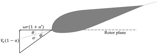
Figure 1.
Direction of velocities at an annular element. Reproduced with permission from [R I Syifa], [2nd international Tropical Renewable Energy Conference (i-TREC) 2017]; published by [IOP Conf. Series: Earth and Environmental Science 105 (2018) 012102], [2018], [5].
The angle between relative velocity and plane of rotation can be determined as [4]:
The angular and axial induction factors can be expressed in terms of lift and drag coefficients [4]:
where —2D lift coefficient; —2D drag coefficient; —combined tip and hub loss correction factor; —radial position of the cross section; —chord length; —number of blades; ω—angular velocity of the wind turbine rotor.
Lift and drag coefficients in Equations (2) and (3) are taken from the 2D airfoil experimental or Computational Fluid Dynamics (CFD) data based on the angle of attack [3].
In the BEM scheme, the blade is first divided into many sections across the span. At each section, Equations (1)–(3) are used in an iterative scheme to calculate the local force (represented by coefficient THRUST) and the local torque (represented by coefficient TORQUE) acting on the annular element.
The BEM method is an iterative technique that helps users to determine a general shape of the blade, i.e., cross-section profile, number of blades, chord distribution and twist distribution, based on some predefined parameters such as maximum power output, rotational speed, wind speed, and rotor radius. After the iteration procedure is completed, the end result can be used to create the 3D geometry of the blade that satisfies the design criteria. This method assumes 2D inviscid flow around the blade elements located along the blade. In real life, wind turbines operate under 3D turbulent aerodynamic conditions which can make the design created by BEM unrealistic or inefficient [6,7,8]. Another drawback of the BEM method is caused by the limited availability of the lift and drag coefficients for various angles of attack and Reynolds numbers. This constrains the number of possible configurations that an engineer can work with. To overcome this limitation, researchers have introduced extrapolation techniques to calculate coefficients for a wider range of angle of attack values using experimental lift and drag coefficients measured at some specific angles of attack [9,10,11].
The design methods described above are normally used for creating wind turbine blades from the ground up. If there is an existing design, a better option is to optimize the design to save time and effort. However, this option may not be readily available. There are a wide variety of optimization studies performed on wind turbine blades using different optimization methods and pursuing different optimization goals. One study used Artificial Neural Network to optimize the National Renewable Energy Laboratory (NREL) Phase VI wind turbine blade to produce a higher power output. The optimized blade showed a 9% increase in power output [12]. A multidisciplinary aero-elastic optimization of the wind turbine used a special optimization toolbox integrating a BEM-based code to minimize mass and improve the structural properties of the blade [13]. Another study optimized a blade under fluid-structure interaction conditions [14]. These researchers used a combination of software packages to perform structural and aerodynamics analysis to optimize blade geometries with sequential two-point diagonal quadratic approximate optimization. A study demonstrated the optimization of a blade using twist angle, chord length, and airfoil shape as variables [15]. They also used a BEM-based code together with an Ant Colony algorithm to search for the optimal shape. Another use of this nature-based optimization algorithm was presented in S. Jelena’s study, which coupled this algorithm with the BEM method to evaluate the aerodynamic performances of a blade, and the Finite Element Method (FEM) was used to calculate its structural properties [16]. The goal of optimization was to minimize tip deflection and mass of the blade. A MATLAB and ANSYS combination to solve the blade optimization problem was utilized in J. Zhu’s study [17]. As in S. Jelena’s study [16], the researchers used BEM and FEM to estimate the aerodynamic and structural performances of a blade. They used a genetic algorithm for the optimization of the blade design with the criteria of maximum energy production and minimum mass. It can be noted that all these studies incorporate the BEM method as a tool for the evaluation of the aerodynamic performance. As it was mentioned in the previous section, the BEM cannot fully account for fully 3D turbulent aerodynamic effects. In addition, pure stochastic approaches can lead to unnecessary waste of computing resources and slow the optimization process, especially without guidance from the flow physics and special rules.
1.2. Stall Delay
One of the effects related to flows in the span-wise direction caused by the rotation of the wind turbine blade is 3D stall delay. This 3D rotating flow around wind turbine blades tends to delay the onset of flow separation [2], thus leading to potential high lift improvement because the local angle of attack can be increased to values greater than the corresponding 2D ones. Therefore, the consideration of the stall delay could improve blade designs. For example, many researchers considered the stall delay effect on the blade surface and derived corrections to convert the 2D lift and drag coefficients into their corresponding 3D-equivalent values to help improve the blade designs using BEM [18,19,20,21,22].
Alternatively, to utilize the stall delay is to incorporate CFD into the design process to directly analyze the complex 3D flow around the blade geometry and the interacting influence on the turbine performance. The findings can then be utilized to optimize the blade geometry by changing the angle of attack and other parameters. The main drawback of this approach is that the calculation of the wind turbine performance using CFD is a highly computing-time-consuming and labor-intensive process. In addition, multiple software packages for solid modeling, mesh regeneration, CFD analysis, data processing/transfer and optimization may need to be utilized. The iterative design optimization process needs to consider the changing blade geometry and computational mesh in the CFD model in each iteration. Repetitive operations of the above optimization process can be an issue for many designers. This approach is not only inefficient but has also limited control over the 3D shape optimization. Commercial CAD packages such as SolidWorks are more suited to 3D design modifications. The bridging of the gap between a sophisticated CAD package and a complex CFD solver is a subject of great interest. To make matter worse, the blade geometry and the CFD analysis results will have to be transferred to an optimization package after each design optimization iteration to determine the new blade geometry.
This work presents two approaches adopted for the optimization study. The first approach proposes a framework that combines the capabilities of the different CAD, CFD, and optimization packages and methods to automate the design optimization process. The proposed framework integrates multidisciplinary 3D parametric modeling, the Inverse Blade Element Momentum (IBEM) method [4], a physics-based optimization scheme and 3D Reynolds-averaged Navier–Stokes (RANS) simulation with a complex turbulent model to iteratively guide the optimization of the blade in order to exploit the 3D stall delay. In the second approach, an integrated goal driven optimization toolbox is adopted, combining CAD and CFD to perform parametric optimization where the individual foil shape is optimized by searching for the optimal trailing-edge angles across the blade to achieve a high-power output.
2. Materials and Methods
2.1. First Approach
Figure 2 shows the proposed automation framework in the first approach, in which there are three major components. The first part is the CAD software. SolidWorks is one of the commonly used CAD packages for blade designs. After the design has been finalized, SolidWorks can output the 3D blade model to the mesh solver for grid generation and regeneration during the optimization of the blade geometry. The second component is the CFD package, which is the ANSYS Fluent software with modules for pre-processing including grid generation, numerical simulation, and post-processing, mainly for verifying the new design in the optimization loop. The third component is the optimization environment where MATLAB was incorporated. It was also chosen as a core component for the automating framework as it can perform data interpretation and optimization using separate scripts as well as communicating between different applications and control the sequence of operations.
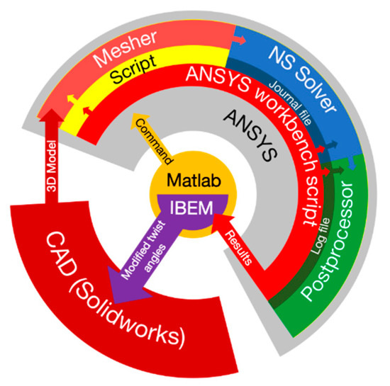
Figure 2.
Schematic representation of the automation framework.
The governing equations for the CFD simulation utilize 3D Reynolds-Averaged Navier-Stokes (RANS) equations in the rotating frame of reference. This set of equations does not include an energy equation as it is assumed that there is no heat transfer, and the flow is considered to be incompressible and steady in the rotating frame. The solver settings can be selected together with the solution schemes in the CFD solver. Similarly, the accuracy for spatial discretization of different parameters can be adjusted. In the first approach, a 3D RANS solver was employed to calculate statistically steady-state 3D turbulent flow over a single blade within a 180° segment with periodic boundary conditions.
Airflow over a rapidly rotating blade is normally 3D and turbulent, therefore, a suitable turbulence model should be selected to model the Reynolds-averaged flow field, which is a simplified and commonly used approach for the analysis of complex 3D turbulent flows in engineering applications. Here the k-ε model with Menter–Lechner near-wall treatment is selected as it is found to be more suitable for flows that involve rotation. Equations (4)–(6) represent this model [23].
where —turbulence kinetic energy due to the mean velocity gradients; —turbulent kinetic energy; —turbulent dissipation; —air viscosity; —air density; —eddy viscosity; —velocity component; —active only at low Reynolds number values; —constants
In the proposed framework, the initial blade design is first generated using SolidWorks. The 3D solid model data are then transferred from SolidWorks into the ANSYS environment using JavaScript add-in through Python script files. Then ANSYS built-in journaling and scripting capabilities are used for processes automation. After the blade import, the meshing process is initiated. The mesh parameters are predetermined prior to initiation from the mesh convergence study. These parameters include mesh inflation layer specifications for the blade wall boundary layers and control parameters for mesh element sizes. Next, the simulation settings, such as boundary conditions and governing equations, are set up via predetermined scripts. The scripts also save the results after simulation is finished. The results come out as pressure distribution data which are exported as CSV files and are used by MATLAB.
2.2. Inverse Blade Element Momentum Method
The outputs from the CFD simulation are used for the optimization of the blades. Numerous optimization schemes for turbine blades have been reported [17,18,19,20,21,22]. These optimization schemes could be progressively implemented individually into the proposed system. This section describes one of the implemented schemes that is very similar to the standard BEM method, which is the Inverse Blade Element Momentum (IBEM) method. It uses force data obtained directly from experiment or simulation to evaluate the lift, drag coefficients, as well as the angle of attack. This helps to include realistic 3D flow effects, such as stall delay, into the blade design improvement and optimization processes.
In the IBEM scheme, the blade is also divided into sections. At each section, the iterative scheme depicted in Figure 3 is used to calculate THRUST and TORQUE can be obtained from either simulation or experiment and are then used to compute , which is a correction factor that includes the hub and tip losses [24,25,26,27,28,29]. The new axial and angular induction factors are then derived and used to check for convergence. Upon convergence, the local 3D lift and drag coefficients (i.e., L,3D and D,3D, respectively) along with the angle of attack are determined for each annular element.
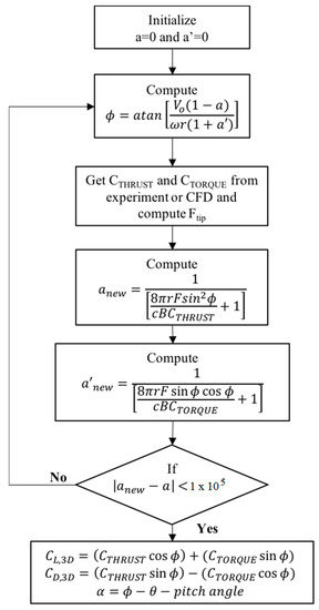
Figure 3.
Inverse Blade Element Momentum (IBEM) method.
The pressure readings from CFD simulation are used to determine THRUST and TORQUE. The IBEM scheme implemented in the proposed system then uses these values to estimate the angle of attack, 3D lift, and drag coefficients at each section. These estimations are then used to find the average lift-to-drag ratio across the blade. The criterion is to maximize the average lift-to-drag ratio for the whole blade. The first step is to search for the location where the maximum lift-to-drag ratio occurs. The angle of attack at this location is used as the reference for the adjustment of the twist angles at all other sections. The magnitude of adjustment for the twist angle at every section is determined by the difference between the local and the reference angles of attack. The twist angles newly determined are then saved and transferred to the 3D parametric modeler to generate a new blade 3D model. The flow of this process is depicted in Figure 4.
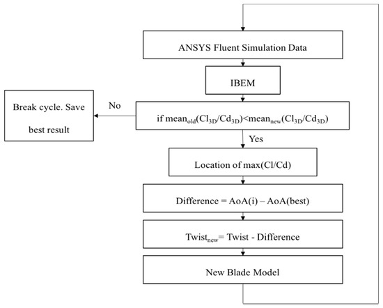
Figure 4.
Optimization scheme using IBEM method.
The 3D model of the turbine blade is generated automatically in SolidWorks using airfoil profiles (S809) at various span-wise locations, which contain the local twist angles and chord lengths, containing global parameters of the model. Their actual values are inferred from the linked external file. By varying the values of the parameters in the linked file, the 3D geometry of the turbine blade can be altered. In the proposed system using the IBEM scheme, the magnitudes of local twist angles are the variables of interest. They are obtained from the IBEM-based optimization scheme together with the chord lengths at different sections and transferred into SolidWorks to generate the new blade geometry. A spline function is then applied to generate a smooth blade model across all the sections.
After SolidWorks generates the new blade 3D model, it is transferred to the CFD package for further aerodynamic evaluation. The process is repeated until an optimal design is obtained. When the process stops, the optimal blade design can be obtained.
2.3. Second Approach
In the second approach, unsteady 3D turbulent flow over the whole rotating rotor was calculated using a 4D Unsteady Reynolds-averaged Navier–Stokes (URANS) solver. The blade is divided into twenty sections (see Figure 5), which is the same as in the first one. The trailing edge in each section is remodeled and its angle is set as an independent design parameter by changing the position of the trailing edge. The distance from the new trailing edge to its original position perpendicular to original chord line is the design parameter as shown in Figure 6.
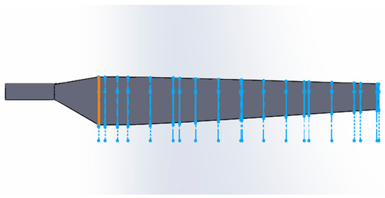
Figure 5.
Blade geometry and location of 20 sections.
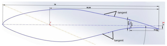
Figure 6.
Cross section geometry.
The embedded optimization tool Design Explorer is adopted in the optimization process, where MISQP (Mixed-Integer Sequential Quadratic Programming) Method is employed. MISQP is a method that solves single objective optimization problems by a modified sequential quadratic programming method and is available for both discrete and continuous input parameters. The design parameter in each section is assigned a specific number from a given parameter set, as shown in Table 1. The second optimization framework and its procedures are graphically illustrated in Figure 7.

Table 1.
Discrete input parameters in parameter set.
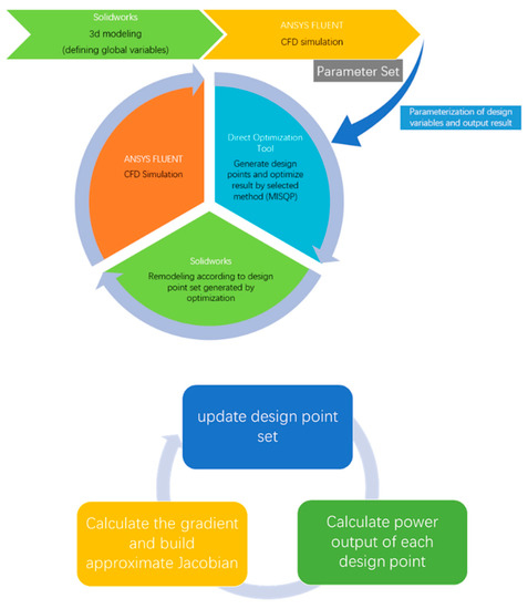
Figure 7.
The second optimization framework.
3. Results
3.1. NREL Phase VI Experiment
The NREL Phase VI rotor blade and its associated experimental data [12] are employed to first validate the implemented CFD codes and numerical models for the prediction of complex 3D turbulent aerodynamics over the blade and the rotor. This blade and the rotor had been wind tunnel tested under various turbine configurations and flow conditions and the experimental data are readily available for this purpose.
The NREL Phase VI wind turbine blade and rotor were modeled in SolidWorks using information provided in the NREL Report [8], from which the Sequence “S” of the blade study series is used. It is characterized by zero yaw angle, no tittering, and the absence of the five-hole probes, to exclude their influence on the fluid flow. The main region of the blade starts at 1.257 m from the hub and ends at 5.029 m. It has a variable twist angle in the span-wise direction based on the NREL s809 airfoil profile. Its chord length decreases toward the end of the blade and the local twist angle changes in the clockwise direction from its root to the tip. The developed 3D models can then be imported into ANSYS.
3.2. 3D RANS
For computational efficiency, the symmetrical and rotational nature of the wind turbine operation is exploited. The ANSYS Fluent MRF functionality and periodic boundary conditions help to simulate the interaction between the rotating blade and incoming air flow efficiently because they allow the use of only one blade for the analysis.
The computational domain is defined by its boundaries, within which the blade is located and would interact with the fluid. The domain developed based on a single blade is shown in Figure 5, which is in the form of a half-cylinder with a radius of 30 m and a total length of 70 m. A small cylindrical cut-off with a radius of 0.51 m is used to replace the presence of the hub. The blade is located 20 m from the inlet and 50 m before the outlet. The origin of the global coordinate system is located at the hub of the wind turbine. Since the simulation is simplified by the use of the half-cylinder domain with imposed rotation around the Z-axis, the two periodic interfaces shown in Figure 5 are used. Previous fluid dynamic studies of the NREL Phase VI wind turbine used different meshing methods and software packages. Nevertheless, it is generally accepted that structured mesh is more economical as it reduces the total number of elements compared to an unstructured one. However, the major drawback of structured meshes is that it requires a great effort to construct. For that reason, an unstructured mesh is used in this work, but the near-wall mesh is structured to improve its resolution of the turbulent boundary layers. Unstructured mesh also requires mesh refinement in the zones where complex fluid flow occurs. This includes blade surface and, to a certain extent, regions surrounding it. The ANSYS Fluent built-in meshing tool can insert face sizing and inflation layers on top of the blade surfaces. In addition, periodic boundary conditions require mesh matching in the regions where rotation will occur. This includes the two bottom faces of the fluid domain shown in Figure 8. The resulting hybrid unstructured/structured mesh is shown in Figure 9. When applying inflation layers, it is important to have a sufficiently small first-layer thickness in order to resolve the laminar sublayers under the generally turbulent boundary layers along the blade surfaces. A thickness of 0.00001 m is used to maintain the Y+ value below 1. This will help to capture any turbulent boundary layer and its separation from the wall accurately.
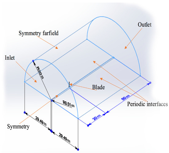
Figure 8.
National Renewable Energy Laboratory (NREL) Phase VI wind turbine and fluid domain and boundary conditions (all dimensions in meters).
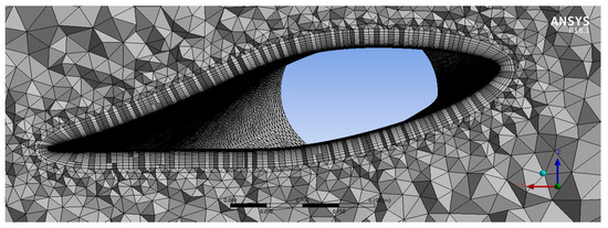
Figure 9.
A sample mesh over the wind turbine blade.
The scheme for spatial discretization of pressure, momentum, and turbulent kinetic energy is second-order accurate with a second-order upwind scheme chosen. A pseudo-transient option with high-order-term relaxation is applied to reduce computational time [23]. The numerical solution method for the incompressible and steady flow is based on a pressure correction scheme. The discretized algebraic equations are solved by an iterative method until a certain level of convergence is reached. As stated above, the k-ε model with Menter–Lechner near-wall treatment turbulence model is used. This turbulence model is best suited for flows with rotation present and previously reported results with the model have shown good agreement with the NREL test data [23].
The boundary conditions and fluid properties are presented in Table 2. The offset of the blades is set at 180° as the wind turbine has only two blades. The rotational speed is 72 RPM. The incoming wind speed ranges between 5 and 25 m/s in the direction perpendicular to the rotating plan, i.e., along the negative Z direction. The inlet boundary condition is set to velocity inlet. The turbulence intensity of the flow is specified as 5%. The outlet pressure has a default gauge pressure of zero Pa. The top surface of the domain or the far field is treated as a symmetry boundary condition. The small cylindrical cutout, which represents the hub of the wind turbine, is also treated as a symmetry boundary condition [24]. The blade surface is defined as a wall with a non-slip condition. The interior of the domain is filled with air, whose physical properties are listed in Table 2.
Table 2.
Boundary conditions and fluid properties.
3.3. 4D URANS
In the second approach, a sliding mesh method is adopted, where the CFD model consists of two bodies, the outer flow domain and a rotating inner body in which the rotor is subtracted. Considering the incompressible nature of the flow, a pressure-based transient solver was adopted, using the finite-volume method for space discretization and semi-implicit time integration of the SIMPLEC solver on 16 CPU cores and the second order upwind scheme was chosen for pressure, momentum, turbulence kinetic energy. The k-ε turbulence model was also used where adaptive wall function was selected. And since the sliding mesh method was adopted in the mesh configurations, a mesh motion with 72 rpm angular velocity was assigned to the rotor domain which is shown in Figure 10 and Figure 11. In boundary conditions, the inlet was chosen as velocity inlet and the wind speed is 10 m/s, normal to the boundary. The cylindrical surface was set as symmetry, which means there is no velocity component that is normal to the cylindrical boundary.
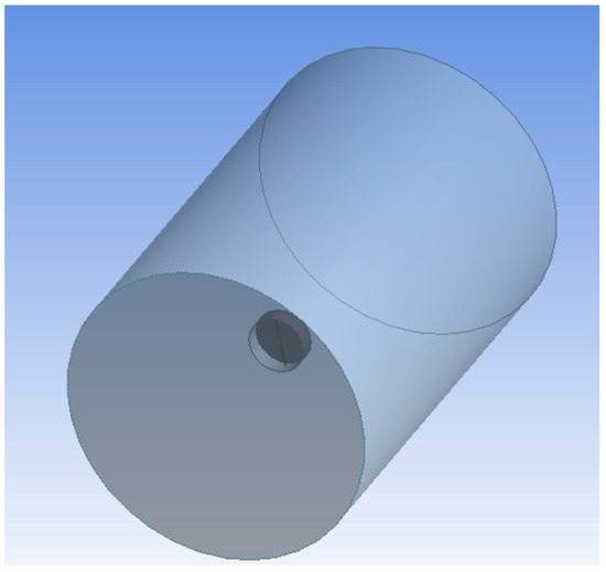
Figure 10.
Multi-blocks for Unsteady Reynolds-averaged Navier–Stokes (URANS) simulation.
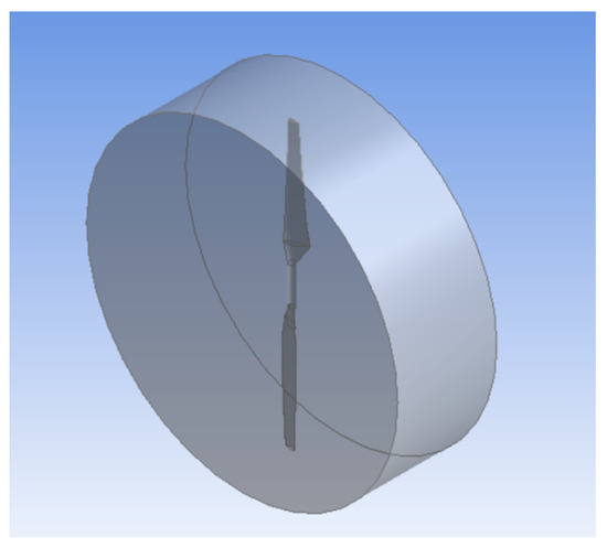
Figure 11.
The rotating block.
3.4. Case Study Results Validation
The mesh convergence study was performed by both approaches. The results of 3D RANS simulation are shown in Figure 12. The mesh refinements have dramatically diminished the change of the power output after 6 million elements were used. Approximately 10 million elements were chosen to be used for this study for extra accuracy of the calculation of the boundary layers and drag force since the drag coefficient was used in the optimization process. One simulation with the given number of elements took approximately 17 h to calculate on the 16-core workstation, with 128 GB of RAM.
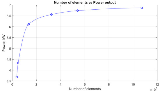
Figure 12.
Mesh convergence analysis.
The numerical analysis was performed on the model at different wind speeds and the pressures obtained were converted to pressure coefficients. The pressure coefficients distributions in different sections are compared with the experimental measurements obtained from the NREL Phase VI experiments. Figure 13 shows the comparison of pressure coefficient distributions at a wind speed of 10 m/s. To account for measurement variations, error bar plots are used. The mean values are highlighted by the “*” sign and variation bars display the upper and lower thresholds values. Red curves represent the results obtained from CFD simulation and the blue stars with bars the actual measurements of NREL tests. Generally, the simulation results are within the range of possible values measured in the experiments. It is noted that discrepancies are especially pronounced close to the leading edge on the suction side of the blade and most notable at the 47 and 63% span stations. Results at other values of wind speed are relatively similar.
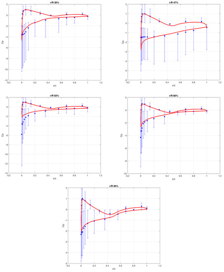
Figure 13.
Pressure coefficient distribution for 10 m/s wind speed: Pressure coefficient at 30% span, Pressure coefficient at 47% span, Pressure coefficient at 63% span, Pressure coefficient at 80% span, Pressure coefficient at 95% span (from left-hand top to right-hand bottom).
In the second approach (4D URANS), the whole rotor model uses 19.8 million elements. Additionally, the 4D URANS simulation took 3.5 h on a 44-core workstation with 516 GB of RAM. The power output of the original design is 8799.24 W which is closer to the experimental data compared to the result of the first approach, as shown in Figure 14.
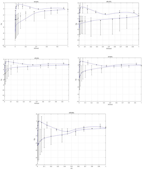
Figure 14.
Pressure coefficients distribution for 10 m/s wind speed.
4. Discussion
In the first approach, the CFD model developed for the NREL Phase VI rotor blade is then employed to validate the proposed optimization framework. The wind speed is set at the designed condition of 10 m/s. Figure 15 shows the distribution of the original blade 3D lift-to-drag coefficient ratio. The highest ratio is located towards the end of the blade, at the last span-wise section. This point is indicated as the highest ratio in Figure 15. This location is the reference point from which the difference between angles of attack will be calculated in the IBEM optimization scheme. The reference point is also shown in Figure 16 for the angle of attack distribution of the original blade. The mean 3D lift-to-drag coefficient ratio across the blade is 8.188.
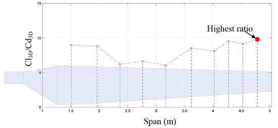
Figure 15.
Cl3D/Cd3D ratio distribution for the original blade at 10 m/s.
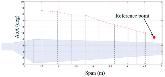
Figure 16.
Angle of attack distribution for the original blade at 10 m/s.
The implemented system is activated with the original blade as the starting point to determine whether the proposed framework with the IBEM-based optimization scheme is able to improve the design. For any design improvement, the optimized design must have an overall mean 3D lift-to-drag coefficient ratio greater than 8.188. The optimized results of the final design obtained are given in Figure 17 and Figure 18.
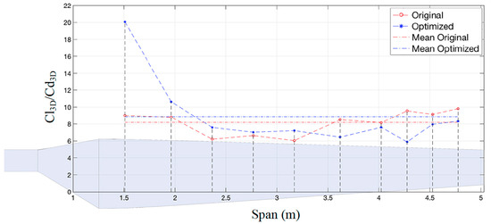
Figure 17.
Cl3D/Cd3D ratio distributions for the original and optimized blades at 10 m/s.
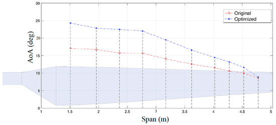
Figure 18.
Angle of attack distribution for the optimized blade at 10 m/s.
The mean 3D lift-to-drag coefficient ratios across the blade for the original and final designs are shown in Figure 17. The IBEM-based optimization raises the mean lift-to-drag ratio across the blade from 8.188 to 8.8734. The comparison between the original and final mean 3D lift-to-drag coefficient ratios in Figure 17 indicates that the ratios of the optimized design remain higher than that for the original blade until around the middle of the blade. After this, the trend is reversed and continues until the tip of the blade.
The angle of attack distributions for the original and final designs are shown in Figure 18. The angle of attack at every span has increased except at the reference point. This is in accordance with the proposed adjustment criteria. The comparison between the original and final angle of attack distributions in Figure 18 indicates that the difference between the angles of attack is more pronounced near the root of the blade. The difference diminishes towards the tip.
Figure 19 shows the comparison of the twist angles between the original and final designs. The final design is more twisted compared with the original one. The optimized blade 3D geometry is automatically constructed within SolidWorks using the twist angles from the optimized design. The contrast between these blade geometries can be observed in Figure 20. The visual difference between them may not be very obvious. The trailing edge is more curved in the middle for the final design. The difference in curvature is clearer in the end view, where the tip of the optimized blade is inclined more towards the first blade section. The findings prove that the optimization process introduced in this work can indeed improve the mean value of the L,3D-to-D,3D ratio across the NREL Phase VI rotor blade.
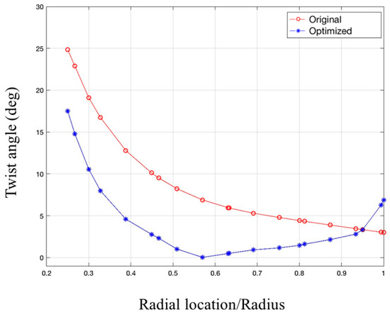
Figure 19.
Comparison of twist angle distributions.
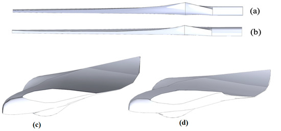
Figure 20.
Side view of the (a) original and (b) optimized blade (top); End view of the (c) original and (d) optimized (bottom).
Although the physics-guided and IBEM-based optimization method is able to optimize the blade efficiently, the overall improvement in the mean value of 3D lift-to-drag ratio is still relatively small. Furthermore, the ratio may drop in some regions. One possible reason for this may be due to how twist angles are adjusted. The modification uses values of fluid flow angle prior to the current iteration stage in the optimization process. It is known that the fluid flow angle is highly dependent on the complex 3D flow characteristics and can be altered by many local factors nonlinearly. Considering the complexity in the determination of the fluid flow angle, it is not straightforward to correctly estimate the magnitude of the next angle of attack at every span section. This leaves room for improvement for the angle adjustment in the implemented scheme. It may be desirable to also consider optimizing the camber simultaneously to further improve the lift-to-drag ratio, which is considered in the second approach.
The results show that the proposed framework as implemented is able to automate the turbine blade design process by integrating CAD, CFD, and optimization packages. The implemented optimization system using the NREL Phase VI rotor blade is able to complete the task after three iterations. This is not surprising as the blade has been reasonably well designed and tested.
Figure 21 shows how the power output of the optimized blade compares to the original one. From these graphs, it is apparent that the original blade is more effective in power generation than the blade with optimized twist angle. It also evident that CFD simulation underpredicts the power output. This means that the maximization of the mean ratio is not enough to increase the overall efficiency of the blade. The reduction of the lift/drag ratio in the second half of the blade suggests that this part has a greater impact on the torque generation. This suggests that it is necessary to use radius-based twist angle correction.
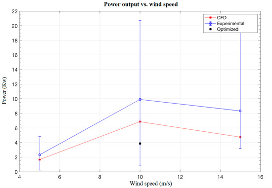
Figure 21.
Power output comparison of the original design (experimental data), CFD simulation, and optimized blade.
Based on the current work, it is envisaged that further improvements and expansions for the toolbox can be planned, such as:
- (1)
- system expansion by implementing more optimization schemes in the form of MATLAB toolboxes;
- (2)
- other CAD, structural dynamics simulation, and CFD packages can be incorporated as well to provide the designer with more choices and capabilities, which can include multiphysics and multivariable optimization;
- (3)
- design can be directly linked to manufacturing by integrating CAD with CAM.
Physics-Based Optimization
Based on the data by MO and Lee (as shown in Figure 22) [28], we can find out what region and what wind speed produce the highest torque. From the root until approximately 60% of the span, the highest torque is produced at 25 m/s; from 60% to 85% of span, the largest torque is generated at 10 m/s and from this point till the tip, the highest torque is produced at 13 m/s. This gives an insight into how to change the twist angle in order to produce a blade that has high torque throughout its span. In order to generate such local twist angles. we need to have the angle of attack data at these speeds. Figure 23 shows the angle of attack (AOA) distributions for multiple values of wind speed. The ones that we are interested in are 25, 10, and 13 m/s. We can deduce the desired twist angles using the formulation presented in Figure 3.
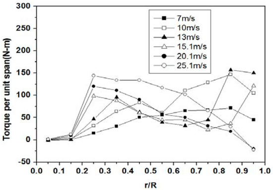
Figure 22.
Torque generated at different radial locations. [Young-Ho LEE], [Journal of Mechanical Science and Technology 26 (1)]; published by [Springer], [2012] [27].
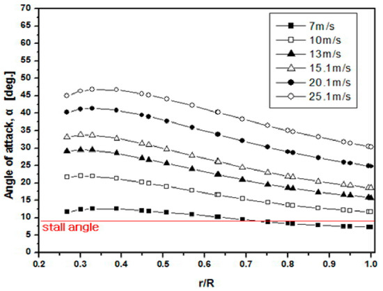
Figure 23.
Angle of attack for different wind speeds. [Young-Ho LEE], [Journal of Mechanical Science and Technology 26 (1)]; published by [Springer], [2012] [27].
There will be three regions of interest along the blade span:
- from 25% until 60%;
- from 60% until 85%;
- from 85% until the tip.
Taking into account the AOA distribution for 10 m/s, we can estimate whether the twist angle should be reduced or increased and by what amount. For the given case and in the first region, the AOA must increase, thus local twist angles must be reduced. The second region must remain the same and for the last region the twist angles must be increased again. The distribution of new twist angle can be changed in three steps. The full step means that angles were changed to desired magnitude, so that they will produce the desired AOA in one iteration. The half-step decreases the twist angle by half the value of the difference and quarterly-step decreases do the same but with a quarter of that value.
The resulting twist angle distributions produced by the aforementioned procedure are presented in Figure 24. It also shows the optimized twist angle distribution based on the original method from Figure 20. The three configurations were simulated using the proposed framework and the calculated AOA are presented in the Figure 25. As can be observed, the AOA follow the prescribed changes. In two regions the AOA becomes higher and in one it remains approximately the same.
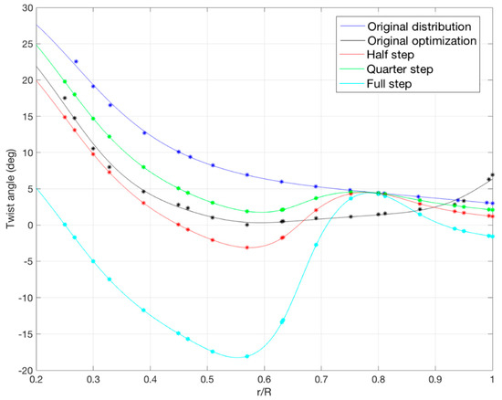
Figure 24.
Twist angle distribution for different blade configurations.
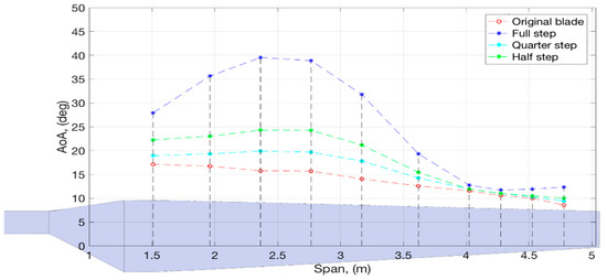
Figure 25.
Angle of attack distribution for different blade configurations.
However, it is shown in Figure 26 that the power output for the adjusted twist angles is lower than the original blade design for almost all cases. Half- and quarter-step changes have shown better performance than the originally optimized blade. The full-step changes even produced a negative torque.
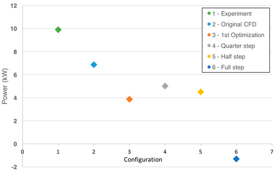
Figure 26.
Power output of the turbine for different twist angle distributions.
It is evident that the proposed radius-based optimization does not produce a more efficient design. Moreover, the power output for this configuration is lower than the original design. This shows that the 3D stall delay is not important for this particular wind turbine blade design.
On the other hand, the results from the second approach in which the trailing-edge design point in 20 sections are changed, as shown in Table 3, show significant improvement in terms of power output. The optimization results are shown in Figure 27. The power output of the optimal design is 9605.65 W, which is 9.6% higher than the original design.
Table 3.
Optimal design points.
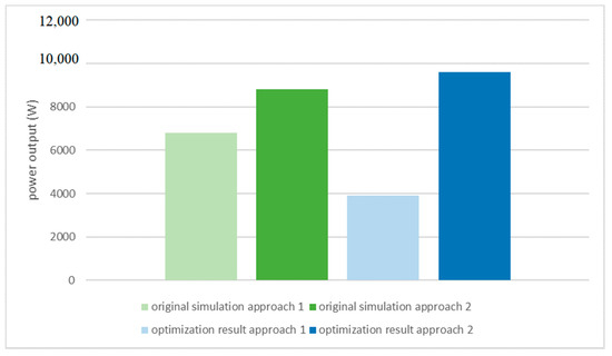
Figure 27.
Comparison of two approaches in terms of power output.
In comparison, the 4D URANS whole rotor simulation is more accurate compared to 3D RANS single blade simulation with periodic boundary conditions, in terms of power output, as shown in Figure 27. Moreover, the results show clearly that changing the twist angle may not deliver better aerodynamic performance if the design does not have prominent enough 3D stall delay. However, the second approach in which the individual trailing edges are modified shows guaranteed significant improvement in power output.
5. Conclusions
The automated design optimization process and the associated toolbox presented in this work show that they can be used to solve complicated blade design optimization problems without human intervention. This is demonstrated by the higher final overall lift-to-drag ratio. The main benefit of using this approach is that it can consider 3D aerodynamic effects such as 3D stall delay, 3D parametric modeling, and physics-based optimization. This opens up many possibilities to improve existing methods and blades by introducing multi-objective and multi-physics optimization methods using different optimization schemes, both deterministic and stochastic. It can also include fluid–structure interaction (FSI) and combined aerodynamic and structural dynamic optimizations.
It was found that the 4D URANS whole rotor simulation in the second approach generates more accurate results than the 3D RANS single blade simulation with periodic boundary conditions in the first one.
By comparing the two approaches, we include that even if the 3D rotational flow plays some kind of role in contributing to the overall aerodynamic performance, modifying the twist angle may not always be sufficient to generate a better outcome since the twist angle or angle of attack of each section has been originally carefully designed for that specific working condition without significant 3D stall delay. On the other hand, the second approach shows greater potential in optimizing the aerodynamic performance with shape modification in the near-trailing-edge region of each blade cross section.
Author Contributions
Conceptualization, Y.Z., S.F., T.S.L.; methodology, S.S., Y.K., Y.Z.; software, S.S., Y.K., Y.Z., S.F., T.S.L.; validation, S.S., Y.K., S.B., Y.Z., S.F., T.S.L.; formal analysis, S.S., Y.K., Y.Z.; investigation, S.S., Y.K., S.B., Y.Z., S.F., T.S.L.; resources, S.S., Y.K., Y.Z.; data curation, S.S., Y.K., S.B., Y.Z., S.F., T.S.L.; writing—original draft preparation, S.S., Y.K.; writing—review and editing, S.S., Y.K., S.B., Y.Z.; visualization, S.S., Y.K.; supervision, Y.Z., S.F., T.S.L.; project administration, Y.Z.; funding acquisition, Y.Z., S.F., T.S.L. All authors have read and agreed to the published version of the manuscript.
Funding
This study is funded by Nazarbayev University through a FDCR grant No. 240919FD3934.
Institutional Review Board Statement
The study was conducted according to the guidelines of the Declaration of Helsinki, and approved by the Institutional Review Board (or Ethics Committee) of Nazarbayev University.
Informed Consent Statement
Not applicable.
Data Availability Statement
Data available in a publicly accessible repository.
Conflicts of Interest
The authors declare no conflict of interest.
List of Abbreviations
| CFD | Computational Fluid Dynamics |
| NS | Navier–Stokes |
| RANS | Reynolds-averaged Navier–Stokes |
| URANS | Unsteady Reynolds-averaged Navier–Stokes |
| IBEM | Inverse Blade Element Momentum |
| AOA | Angle of Attack |
| BEM | Blade Element Momentum |
| CAD | Computer Aided Design |
| NREL | National Renewable Energy Laboratory |
| FEM | Finite Element Method |
| MRF | Moving Reference Frame |
| COM | Component Object Model |
| API | Application Programming Interface |
| CSV | Comma Separated Value |
References
- Global Wind Energy Council. Global Wind Energy Council. Retrieved 23 November 2020. 2020. Available online: https://gwec.net/ (accessed on 23 November 2020).
- Syed Ahmed Kabir, I.; Ng, E. Insight into stall delay and computation of 3D sectional aerofoil characteristics of NREL phase VI wind turbine using inverse BEM and improvement in BEM analysis accounting for stall delay effect. Energy 2017, 120, 518–536. [Google Scholar] [CrossRef]
- Manwell, J.; McGowan, J.; Rogers, A. Wind Energy Explained; John Wiley & Sons: Hoboken, NJ, USA, 2011. [Google Scholar]
- Guntur, S.; Sørensen, N. An evaluation of several methods of determining the local angle of attack on wind turbine blades. J. Phys. Conf. Ser. 2014, 555, 012045. [Google Scholar] [CrossRef]
- Pratilastiarso, J.; Nugroho, S.; Tridianto, E.; Syifa, R.I. Experimental study on horizontal axis wind turbine with splitted winglets. IOP Conf. Ser. Earth Environ. Sci. 2018, 105, 012102. [Google Scholar] [CrossRef]
- Glauert, H. Airplane Propellers. In Aerodynamic Theory; Durand, W.F., Division, L., Eds.; Springer: New York, NY, USA, 1935; Volume IV, pp. 169–360. [Google Scholar]
- Hansen, M. Aerodynamics of Wind Turbines; Routledge: Abingdon, UK, 2015. [Google Scholar]
- Hand, M.; Simms, D.; Fingersh, L.; Jager, D.; Cotrell, J.; Schreck, S.; Larwood, S. Unsteady Aerodynamics Experiment Phase VI: Wind Tunnel Test Configurations and Available Data Campaigns; National Renewable Energy Lab.: Golden, CO, USA, 2001. [Google Scholar] [CrossRef]
- Viterna, L.; Corrigan, R. Fixed Pitch Rotor Performance of Large Horizontal Axis Wind Turbines; Scientific & technical information; NASA: Washington, DC, USA, 1982. [Google Scholar]
- Lanzafame, R.; Messina, M. Fluid dynamics wind turbine design: Critical analysis, optimization and application of BEM theory. Renew. Energy 2007, 32, 2291–2305. [Google Scholar] [CrossRef]
- Tangler, J.; Kocurek, D. Wind Turbine Post-Stall Airfoil Performance Characteristics Guidelines for Blade-Element Momentum Methods. In Proceedings of the 43Rd AIAA Aerospace Sciences Meeting and Exhibit, Reno, NV, USA,, 10–13 January 2005. [Google Scholar] [CrossRef]
- Elfarra, M.; Sezer-Uzol, N.; Akmandor, I. NREL VI rotor blade: Numerical investigation and winglet design and optimization using CFD. Wind Energy 2013, 17, 605–626. [Google Scholar] [CrossRef]
- Pavese, C.; Tibaldi, C.; Zahle, F.; Kim, T. Aeroelastic multidisciplinary design optimization of a swept wind turbine blade. Wind Energy 2017, 20, 1941–1953. [Google Scholar] [CrossRef]
- Kim, D.; Lim, O.; Choi, E.; Noh, Y. Optimization of 5-MW wind turbine blade using fluid structure interaction analysis. J. Mech. Sci. Technol. 2017, 31, 725–732. [Google Scholar] [CrossRef]
- Tahani, M.; Maeda, T.; Babayan, N.; Mehrnia, S.; Shadmehri, M.; Li, Q.; Fahimi, R.; Masdari, M. Investigating the effect of geometrical parameters of an optimized wind turbine blade in turbulent flow. Energy Convers. Manag. 2017, 153, 71–82. [Google Scholar] [CrossRef]
- Jelena, S.; Zorana, T.; Marija, B.; Ognjen, P. Rapid multidisciplinary, multi-objective optimization of composite horizontal-axis wind turbine blade. In Proceedings of the 2016 International Conference Multidisciplinary Engineering Design Optimization (MEDO), Belgrade, Serbia, 14–16 September 2016. [Google Scholar] [CrossRef]
- Zhu, J.; Cai, X.; Gu, R. Multi-Objective Aerodynamic and Structural Optimization of Horizontal-Axis Wind Turbine Blades. Energies 2017, 10, 101. [Google Scholar] [CrossRef]
- Snel, H.; Houwink, R.; Bosschers, J. Sectional Prediction of Lift Coefficients on Rotating Wind Turbine Blades in Stall; ECN-C–93-052; ECN: Petten, The Netherlands, 1994; pp. 5–17. [Google Scholar]
- Wang, Q.; Xu, Y.; Song, J.; Li, C.; Ren, P.; Xu, J. 3D stall delay effect modeling and aerodynamic analysis of swept-blade wind turbine. J. Renew. Sustain. Energy 2013, 5, 063106. [Google Scholar] [CrossRef]
- Chaviaropoulos, P.; Hansen, M. Investigating Three-Dimensional and Rotational Effects on Wind Turbine Blades by Means of a Quasi-3D Navier-Stokes Solver. J. Fluids Eng. 2000, 122, 330–336. [Google Scholar] [CrossRef]
- Lindenburg, C. Investigation into Rotor Blade Aerodynamics; Paper ECN-C-03-025; ECN: Petten, The Netherlans, 2003; pp. 53–58. [Google Scholar]
- Sørensen, J. The Tip Correction. In Research Topics in Wind Energy; Springer International Publishing: Cham, Switzerland, 2015; pp. 123–150. [Google Scholar] [CrossRef]
- ANSYS FLUENT 18.1 Documentation. Available online: https://www.ansys.com/products/fluids/ansys-fluent (accessed on 23 November 2020).
- Song, Y.; Perot, J. CFD Simulation of the NREL Phase VI Rotor. Wind Eng. 2015, 39, 299–309. [Google Scholar] [CrossRef]
- Mahu, R.; Popescu, F. Nrel Phase Vi Rotor Modeling and Simulation Using Ansys Fluent 12.1. Math. Model. Civ. Eng. 2011, 7, 185–194. [Google Scholar]
- 2016 SOLIDWORKS API Help-Welcome. Help.solidworks.com. Retrieved 23 November 2020. 2020. Available online: http://help.solidworks.com/2016/English/api/sldworksapiprogguide/Welcome.htm (accessed on 23 November 2020).
- Ansys Workbench Mechanical User Guide. Portal-02.theconversionpros.com. Retrieved 23 November 2020. 2020. Available online: http://portal02.theconversionpros.com/ansys_workbench_mechanical_user_guide.pdf (accessed on 23 November 2020).
- Mo, J.; Lee, Y. CFD Investigation on the Aerodynamic Characteristics of a Small-Sized Wind Turbine of NREL PHASE VI Operating with a Stall-Regulated Method. J. Mech. Sci. Technol. 2012, 26, 81–92. [Google Scholar] [CrossRef]
- Moriarty, P.; Hansen, A. AeroDyn Theory Manual; Technical report NREL/TP-500-36881; National Renewable Energy Lab.: Golden, CO, USA, 2005; pp. 9–10. [Google Scholar]


Publisher’s Note: MDPI stays neutral with regard to jurisdictional claims in published maps and institutional affiliations. |
© 2021 by the authors. Licensee MDPI, Basel, Switzerland. This article is an open access article distributed under the terms and conditions of the Creative Commons Attribution (CC BY) license (https://creativecommons.org/licenses/by/4.0/).