1. Introduction
In many industrial applications, such as oil recovery [
1], food processing, coating, and the transfer of crude oil in pipe-like paths [
2], a fluid is injected to displace another fluid in the desired direction. For example, injecting a hydrocarbon solvent or carbon dioxide to displace crude oil in a reservoir can significantly enhance oil recovery. Similarly, displacing water-based polymer muds, nail polish, silicone oil, ketchup, whipped cream, and corn-starch water solution, which are power-law non-Newtonian fluids, is of paramount interest. Using a Newtonian fluid such as water to displace these non-Newtonian fluids may produce an immiscible mixture with a complex interface between the fluids, which is rarely addressed in the literature.
Injection of a fluid with a low viscosity into a highly viscous fluid can create a two-layer/two-core annular flow in the pipe. Depending on the miscibility [
3,
4,
5] or immiscibility [
6,
7,
8] of the displacement, the occurrence of interfacial instabilities (such as the Kelvin–Helmholtz instability) is inevitable. Goyal and Meiburg [
9] investigated miscible displacements of highly viscous fluids by other fluids. They observed that increasing flow rate could turn two-dimensional instabilities (caused by the shear stress between the two fluids) into three-dimensional instabilities. This result is in good agreement with laboratory [
10] and theoretical [
11] investigations. Taghavi et al. [
12,
13] numerically and experimentally investigated miscible displacement flows in low flow rates to analyze the interfacial instabilities triggered in exchange flows. Sahu et al. [
14] analyzed the impacts of inclination angle and dimensionless numbers on the miscible displacement of a fluid by another lighter and less viscous fluid. The observation of tiny instabilities in such flows was in good agreement with their previous studies analyzing the linear stability of fingering structures [
15]. Yang and Yortsos [
16] studied miscible Stokes flows between parallel plates and showed that increasing the viscosity ratio intensifies fingering instabilities and reduces displacement efficiency. In conclusion, the findings indicate that a higher viscosity of the injected fluid can stabilize the fingering structure. However, by lowering the viscosity of the invading fluid, the flow becomes unstable. As a result, roll-up structures are observed in miscible displacements [
17,
18], while sawtooth structures occur in immiscible displacements [
19].
On the other hand, Dimakopoulos and Tsamopoulos [
20] studied the displacement of viscoplastic fluids by air and evaluated the residual wall layer left unyielded at the corners of convergent channels. Papaioannou et al. [
21] analyzed air-displaced viscoplastic fluids and described the conditions required to separate the injected fluid from channel walls. Ebrahimi et al. [
22] and Wielage and Frigaard [
23] studied the displacement of Bingham fluids by other fluids possessing the same densities and investigated the thickness of the static wall layers for different Bingham numbers. Frigaard and Nouar [
24] studied the effects of viscosity models [
25,
26,
27] on the flow dynamics, and they showed the advantages of using the Papanastasiou model over other models to accurately simulate the problem.
In recent years, multiple studies have been conducted to simulate immiscible flows using a multi-component model of the lattice Boltzmann method (LBM) called Shan–Chen [
28,
29]. Auto-separation of phases, less computational cost, more effortless coding, and local calculation of shear rates are the advantages of utilizing the lattice Boltzmann method over other numerical approaches such as smoothed particle hydrodynamics [
30,
31,
32] and finite element [
33]. However, the Shan–Chen model is not capable of simulating fluids with different densities in displacement flows. Moreover, when very low Reynolds numbers are imposed, interfacial instability cannot be observed. Redapangu et al. [
19] used the model offered by He et al. [
34] to improve the accuracy of other studies and investigate displacement flow for two immiscible Newtonian fluids at medium Reynolds numbers. Finally, they succeeded in observing sawtooth-structure instabilities at the interface of the two fluids. It is worth noting that despite the promising advantages of this numerical method over other numerical approaches, it is not capable of modeling displacement flows with high density ratios and its stability at high Mach numbers is a controversial issue.
Although the dynamics of generated finger-like structures have been simulated in both miscible and immiscible states, the displacement of non-Newtonian fluids by other fluids has rarely been investigated. Due to the widespread industrial application of non-Newtonian displacement flows and considerable difficulties in the mathematical description of the fluid–fluid interface, numerical simulation of these problems requires special attention. This study’s primary purpose is to analyze the complicated displacements of water-based polymer muds, which are better described by the power-law equation than any other two-parameter model describing their viscosity. Therefore, the investigation of power-law fluids displacement caused by the injection of Newtonian fluids is the key focus.
The importance of this research is related to the widespread application of pseudoplastic and dilatant fluids displacement by Newtonian fluids (e.g., water) in industrial processes. The compatibility factor and power-law index in the viscosity determination function of these fluids play a crucial role in regulating the resisting forces against the invading fluid movement. Hence, we used the He–Chen–Zhang model, which enabled us to perform the simulation for a wide range of viscosity ratios and evaluate the impact of these factors on the flow behavior without any simplification. Moreover, two groups of figures are presented to exhibit the displacement efficiency and the apparent flow shape. These figures show the displacement efficiency in each longitudinal and cross-sectional area of the channel, the development of interfacial instabilities, and the amount of displaced fluid over time. Then, the injected fluid’s tendency to move toward particular parts of the channel was analyzed. Assessment of this tendency is helpful to provide guideline for reducing the thickness of the static residual layer left on the channel walls.
2. Methodology
A 2D channel was initially filled with a stagnant incompressible Newtonian fluid, Fluid 2, with a viscosity of
and density of
. Fluid 2 was immiscibly displaced by Fluid 1, which possesses a viscosity of
and density of
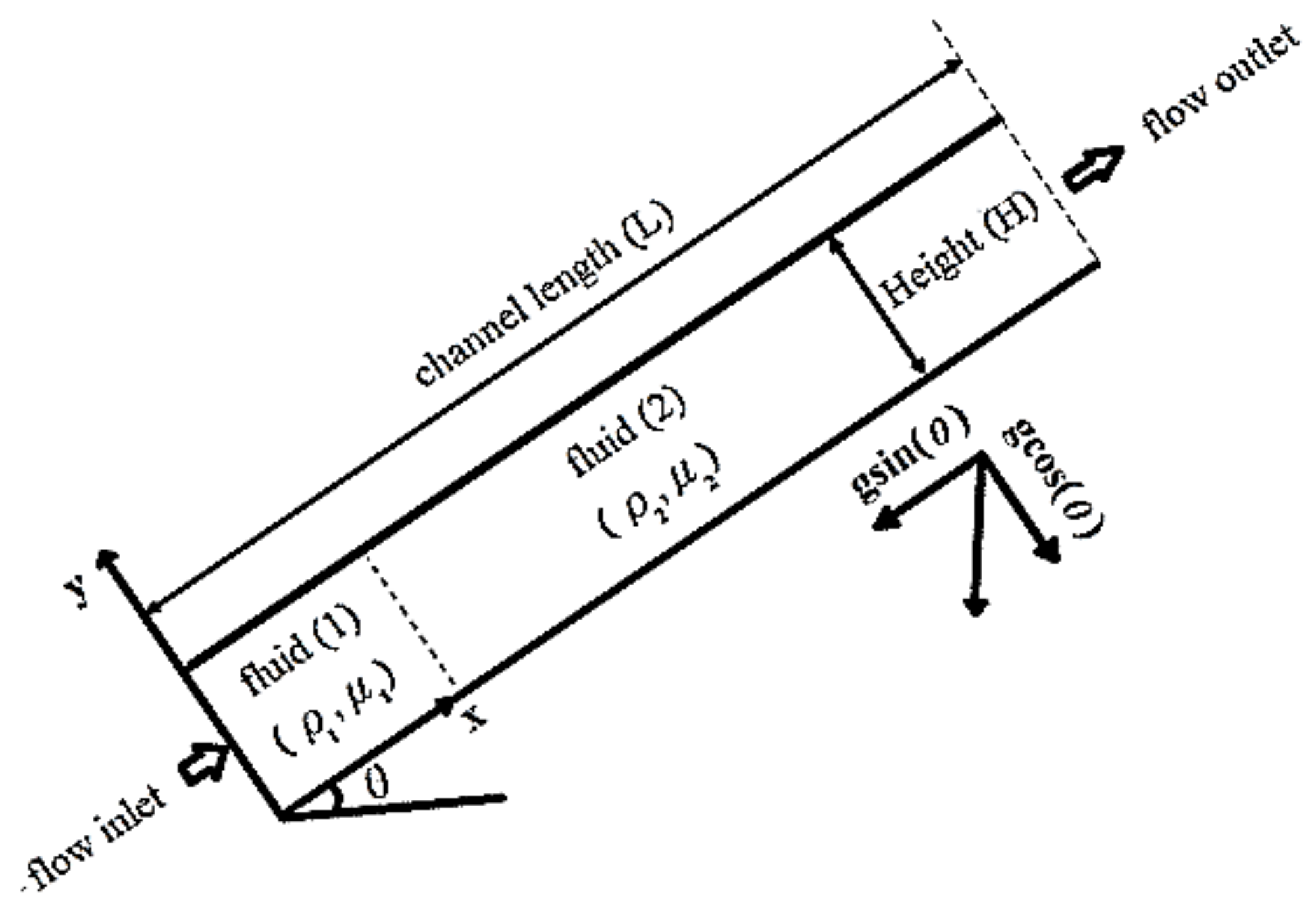
. As shown in
Figure 1, the inlet, outlet, upper wall, and lower wall of the channel are located at
x = 0,
x =
L,
y = 0, and
y =
H, and the channel’s height-to-length ratio is considered to be 1/30. A hydrodynamic boundary condition was used at the upper and lower walls of the channel. Additionally, a developed velocity profile and a Neumann boundary condition for the pressure (by extrapolating) were applied at the inlet and outlet.
2.1. Numerical Approach
A particular version of the He–Chen–Zhang method [
35,
36], developed by Sahu and Vanka [
37] for fluids with unequal viscosities, was employed in this study, and it is described briefly in this section. The two distribution functions (
f and
g) are defined in the collision step as:
where
u and
represent the velocity vector and relaxation time, respectively. The relaxation time is calculated by
as a function of kinematic viscosity.
is the lattice speed of sound in which
is the lattice speed, and
and
are the grid spacing and time step, respectively. The value of
is 1/3. The mesoscopic velocity at the lattice scale is calculated by:
The values of weight functions are listed below:
The equilibrium values of the distribution functions are obtained as follows:
The index function,
, pressure,
P, and velocity,
u, are calculated using:
To calculate the density,
, and kinematic viscosity,
, the following relationships are utilized:
where the subscripts of 1 and 2 represent the properties of Fluid 1 and 2. The values of the index functions for the heavy and light fluids are 0.2508 and 0.02381, respectively.
in Equation (1) plays a crucial role in phase separation and the determination of intramolecular interactions between non-ideal fluids. This function can be calculated using the Carnahan–Starling equation [
38,
39,
40,
41].
where
a determines the magnitude of intermolecular interactions, and its critical value is 3.53357. It means that if
a is greater than this value, the generated flow remains immiscible. It is worth noting that choosing larger values of
a can violate solution convergence. In this study,
a is set to 4, and the fourth-order compact scheme is utilized to discretize
while the second-order discretization is used to calculate
.
Surface tension and gravitational forces are computed using:
where
is defined by
, and
k determines surface tension intensity, which is obtained by:
where
is the direction perpendicular to the contact surface.
2.2. Enforcing Boundary Conditions
The Zou–He boundary condition [
42] used to calculate unknown distribution functions at boundaries is not consistent with the approach of the He–Chen–Zhang method to obtain the macroscopic characteristics of a fluid. Noble et al. [
43] proposed hydrodynamic boundary conditions as a different kind of bounce-back boundary conditions. Based on this approach, a no-slip boundary condition was used to find unknown distribution functions in this paper. The most straightforward way of applying hydrodynamic boundary conditions is to assume equilibrium conditions at the walls, and then the streaming process should take place. Therefore, the streaming distribution functions should not be replaced by the distribution functions at the walls, and all the distribution functions should be set to their equilibrium values. Known values for the density and velocity can possibly be used to compute equilibrium distribution functions at the walls. Guo et al. [
44] developed the boundary condition presented by Chen et al. [
45] to introduce a special kind of boundary condition in which the non-equilibrium part of distribution functions in internal points is extrapolated and added to its equilibrium value at boundaries to obtain values of distribution functions. This method is of second-order accuracy. Finally, in the present study, we used a particular kind of hydrodynamic boundary condition based on the ghost fluid approach and extrapolation of the non-equilibrium values of distribution functions. This approach is also of second-order accuracy and is explained below. By placing walls between lattice points and applying zero gradients to the index functions,
, the index function is obtained as:
where
Nx + 1 and
Ny + 1 are the number of points in the lattice in the directions of x and y. Velocities are reflected in mirror forms to impose non-slip and non-penetration conditions as:
where
and
are the tangential and vertical velocities of the wall, which are assumed to be zero. Distribution function,
f, and pressure are given by:
This pressure is used to compute the equilibrium value of the distribution function, g. Additionally, the substituted velocity in this function must be zero, which leads to its ghost value being ignored. By adding non-equilibrium values to the equilibrium values, it is feasible to calculate g like f in Equation (24).
On the other hand, in hydrodynamic problems, boundary conditions are usually given for macroscopic properties (e.g., velocity and pressure) while values of distribution functions are required at boundaries in the lattice Boltzmann method. A comprehensive strategy is required to compute distribution functions as a function of macroscopic values. Therefore, to obtain unknown distribution functions at boundaries with known velocities or pressures, the extrapolation method can be used. This approach is similar to hydrodynamic boundary conditions except, in the streaming step, distribution functions in internal points should be moved toward walls and replaced [
46].
2.3. Modeling of Non-Newtonian Fluids
Time-independent non-Newtonian fluids have no memory of their motion, and their uniform shear behavior can be expressed as:
where
, and
represent shear stress and shear rate, respectively. The subscript
yx underlines the direction of the stress in the fluid. For these fluids, either the curve of shear stress vs. shear rate (
) does not pass through the coordinate system’s origin, or shear stress may be a nonlinear function of shear rate [
47,
48,
49]. Accordingly, the apparent viscosity (
) is not constant. The behavior of time-independent non-Newtonian fluids can be categorized into three types:
The apparent viscosity of power-law materials, as a general non-Newtonian fluid, is obtained by [
50,
51,
52]:
where
n and
are the power-law index and compatibility coefficient, respectively.
is the magnitude of the shear rate tensor, calculated by:
For
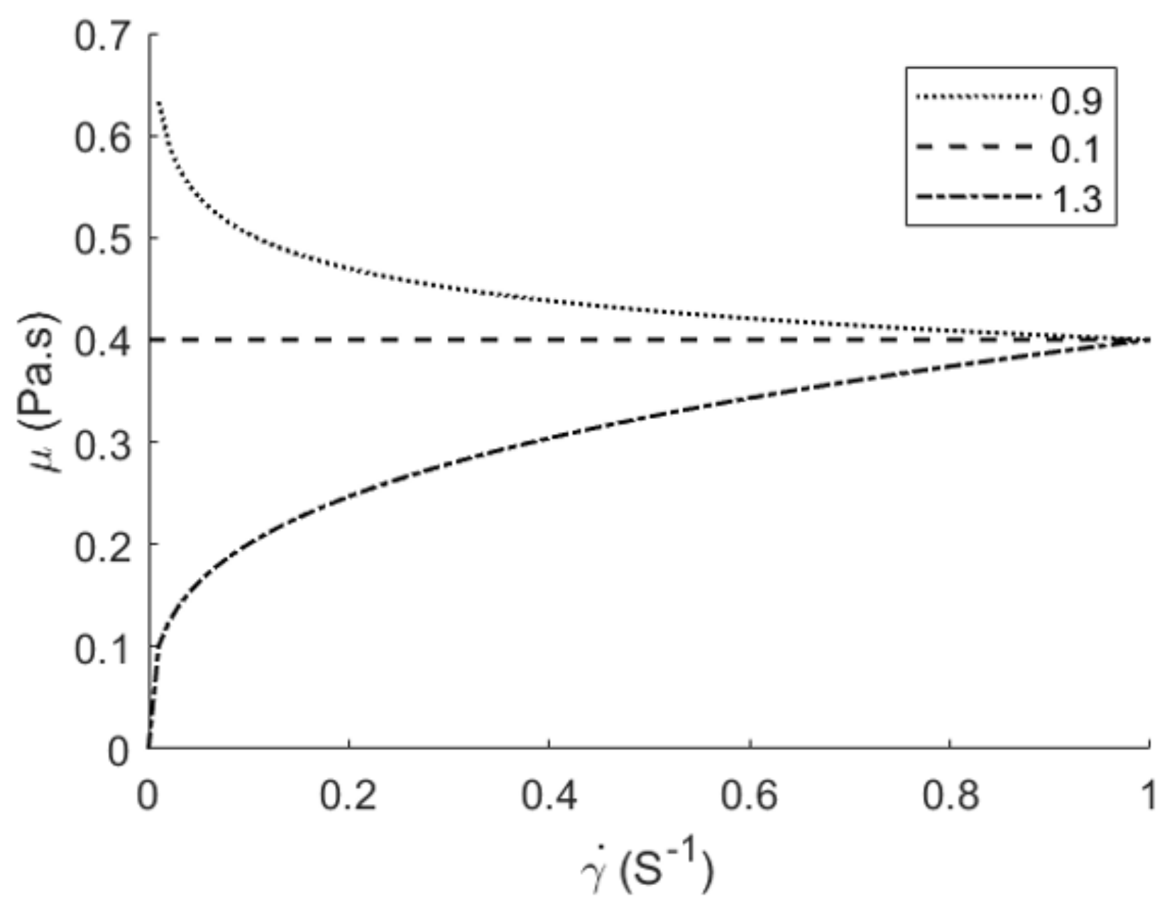
n = 1, the compatibility coefficient is equivalent to the fluid viscosity, and the fluid behaves as a Newtonian fluid. If
, by increasing the shear rate, the apparent viscosity decreases, and the fluid will have thinning behavior. Finally, if
, by increasing the shear rate, the apparent viscosity increases, and the fluid exhibits dilatant behavior. For high shear rates, the apparent viscosity is equal to the constant value of
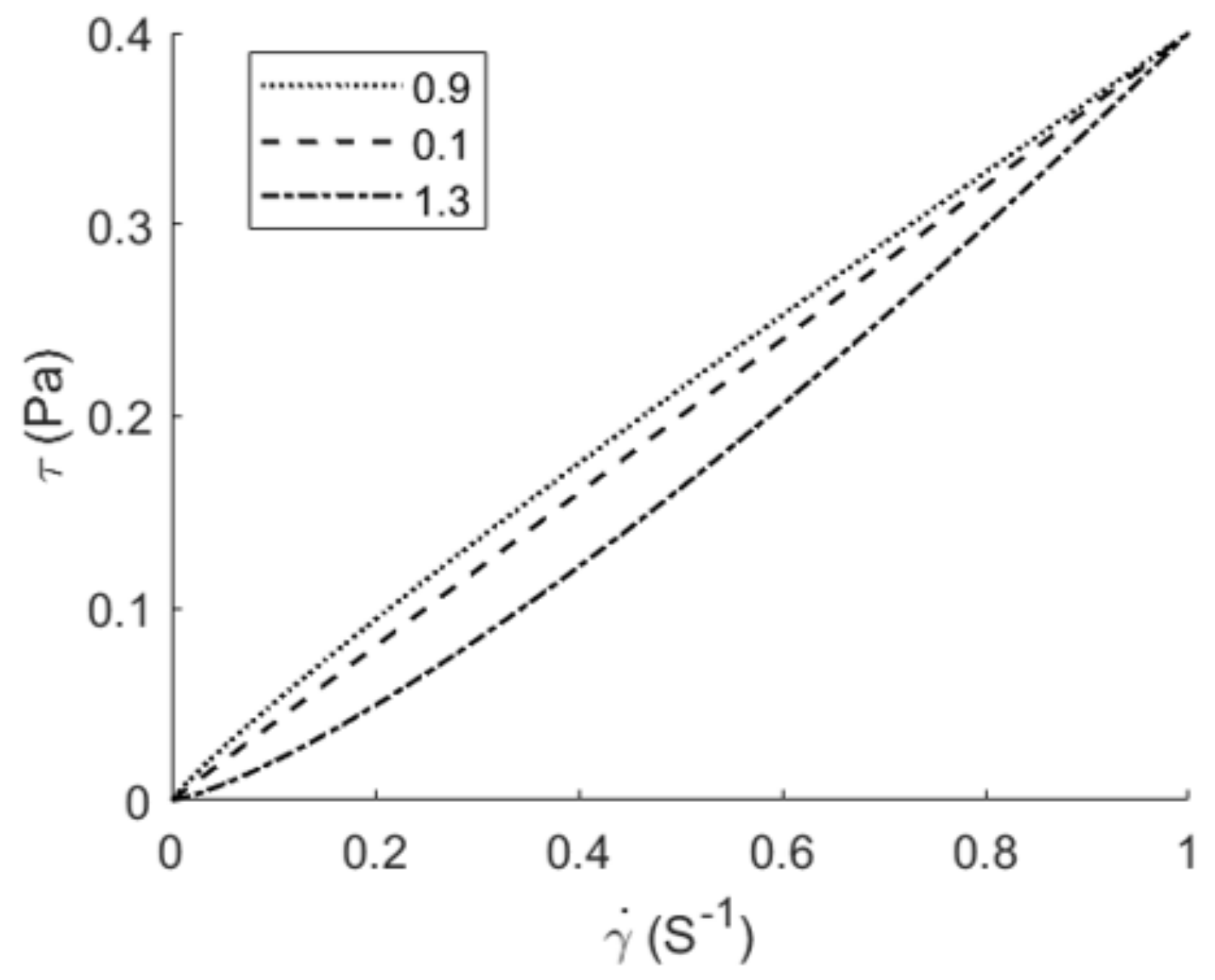
, and the relationship between the shear rate and shear stress becomes linear. Regardless of the power-law index, shear rate growth causes an upward trend in fluid stress as shown in
Figure 2. These trends have different behaviors in terms of concavity, which is the main reason for variations in the viscosity of non-Newtonian fluids as a function of shear rate (
Figure 3).
In LBM, for Newtonian fluids, the relaxation time, which is a function of viscosity, possesses a constant value at any point of the lattice. However, the relaxation time of non-Newtonian fluids at each lattice point is different due to variable viscosity.
3. Numerical Modeling
3.1. Code Validation
Based on the He–Chen–Zhang method and 9-speed square lattices, a multi-purpose code was developed in FORTRAN 95 to simulate immiscible multiphase flows in 2D. The possibility of imposing hydrodynamic, bounce back, slip, no-slip, fully developed, and open boundary conditions enabled us to implement the code for modeling a large variety of multiphase flows. Using this numerical tool and the He–Chen–Zhang method to simulate the problem of this study reduced the simulation time to less than 7 h, whereas it might take a few days if other computational fluid dynamics methods were used.
In this study, the following non-dimensional numbers are used to explain flow behaviors: Reynolds (
), Atwood (
)), viscosity ratio (
), Richardson (
) and capillary (
), where
Q is the volumetric flow rate per unit length,
H the channel width,
g the gravity acceleration, and
is the surface tension in the lattice. Dimensionless time is also defined as
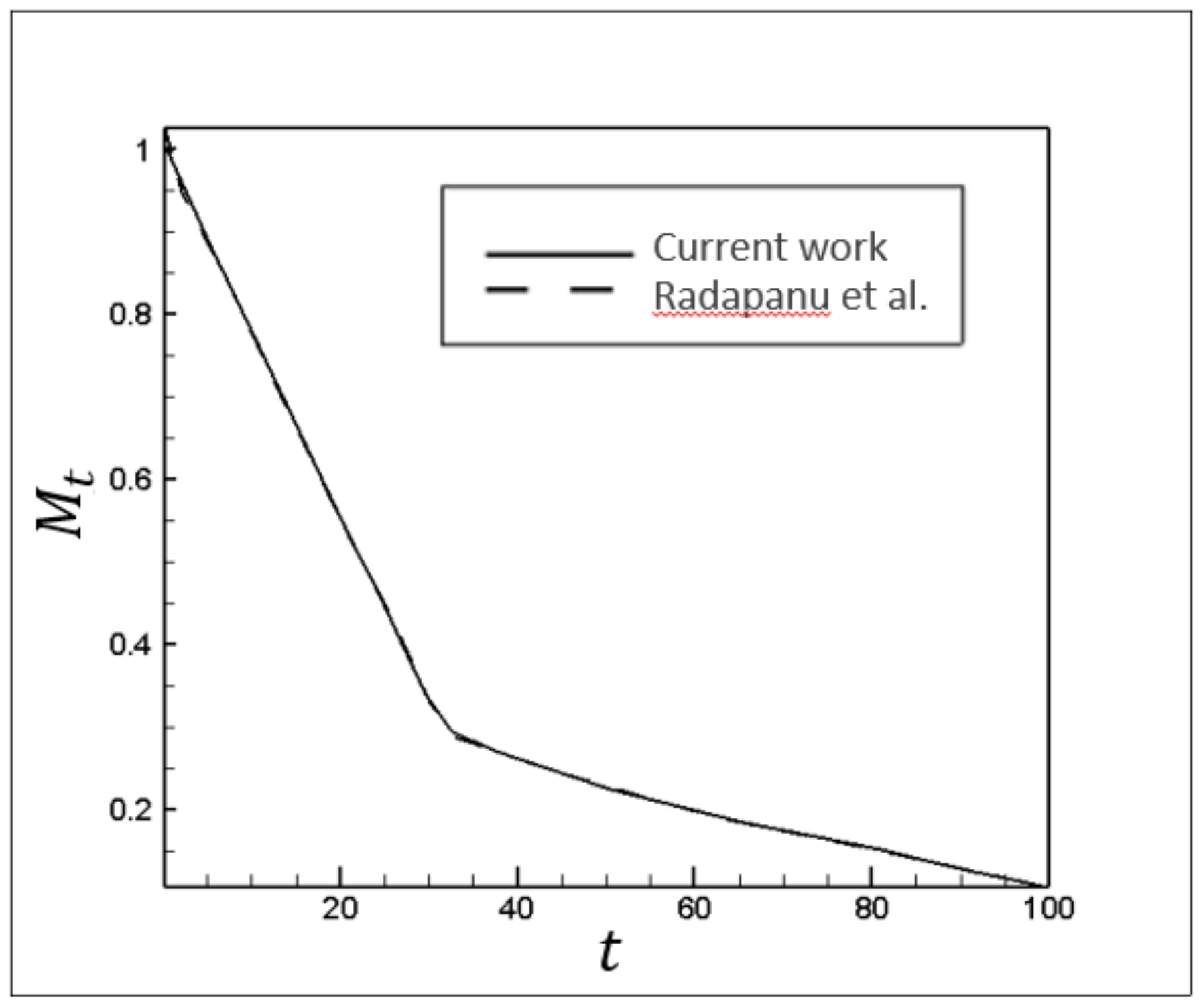
. The developed code was validated against the results of a study by Redapangu et al. [
19] for a simple Newtonian displacement in a horizontal channel with
At = 0,
m = 2,
Ri = 0,
Ca = 0.263, and
Re = 100, as shown in
Figure 4.
3.2. Lattice Layout Study
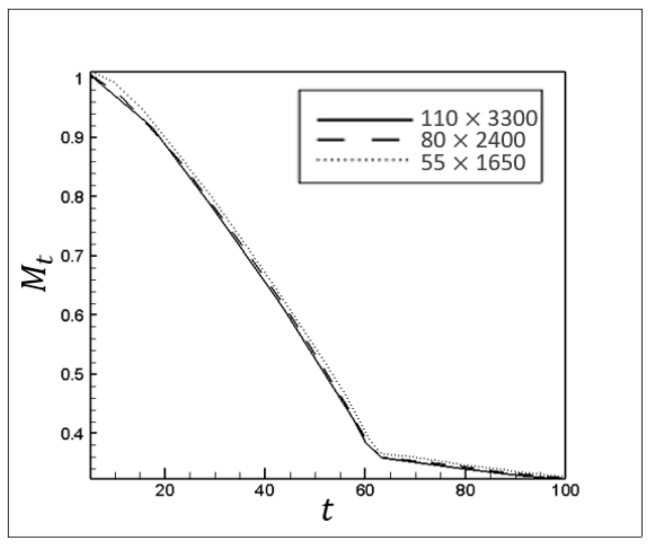
The independence of the results from lattice size was studied for the geometry and configuration shown in
Figure 1.
Figure 5 shows the dimensionless volume of Fluid 2 (
) for
At = 0.2,
m = 2,
Ri = 0.1,
Ca =
,
Re = 100, and
= 45 in the three lattice layouts; 55 × 1650, 80 × 2400, and 110 × 3300.
S is the dimensionless time, and
and
are criteria for the initial and time-varying volumes of Fluid 2, respectively, which are calculated by:
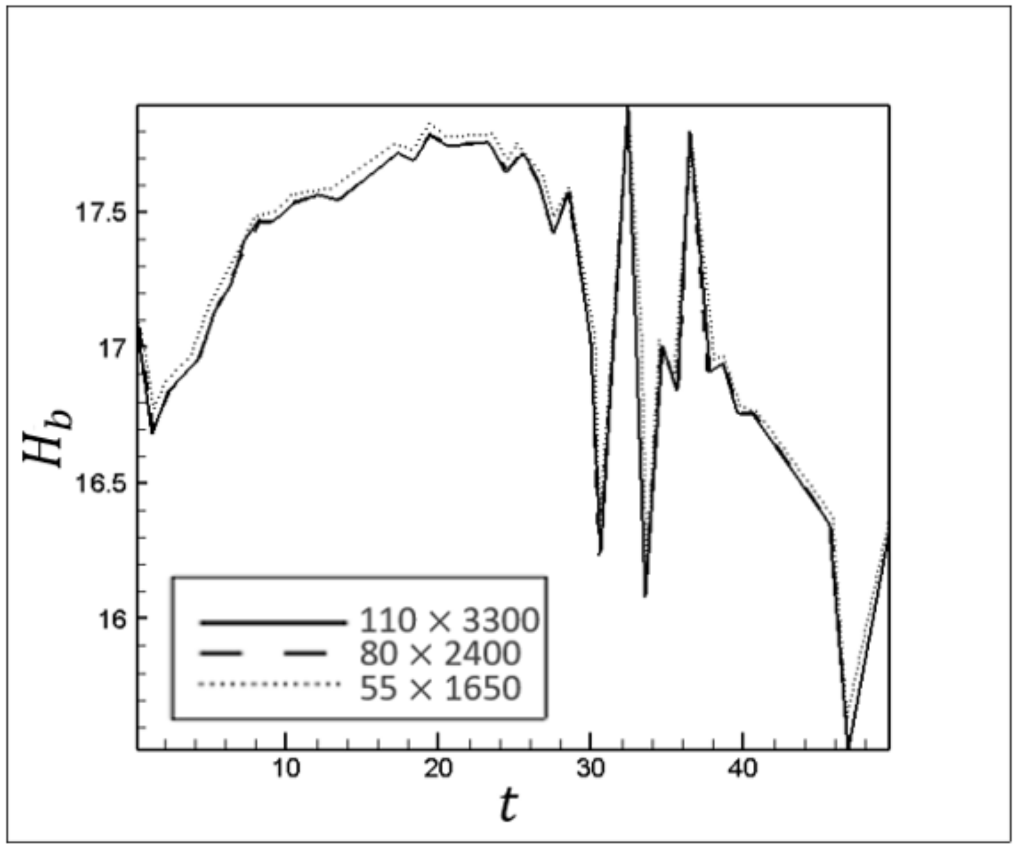
Figure 6 shows the alteration in the mean thickness of the static layer left on the lower wall of the channel for
At = 0.2,
m = 20,
Ri = 1,
Ca =
,
Re = 100, and
= 45. The following equations were used to evaluate these thicknesses at the lower and upper walls, respectively. Eventually, due to the negligible difference between the results of the two denser layouts (110 × 3300) was selected for this study.
3.3. Numerical Procedure
After the initialization of distribution functions, it is necessary to calculate the new relaxation time for the next time step in each iteration by calculating the velocity gradient. In the initial time steps, it is probable that there will be a zero velocity gradient at some points. Furthermore, the velocity gradient at the center of the channel may approach zero in the non-Newtonian fluid. Accordingly, a small value, , is added to the velocity gradient to avoid singularity in Equation (27). In general, the required steps for progressing a time step are as follows:
- (1)
Initialization of distribution functions and relaxation time;
- (2)
Calculation of the macroscopic velocity and density;
- (3)
Calculation of equilibrium distribution functions;
- (4)
Calculation of the velocity gradient;
- (5)
Calculation of viscosity using the structural equation of non-Newtonian fluids;
- (6)
Calculation of the new relaxation time for non-Newtonian fluids;
- (7)
Calculation of new distribution functions in the collision step;
- (8)
Streaming distribution functions toward their adjacent points (propagation step);
- (9)
Calculation of a new relaxation time, velocity field, and distribution functions for the next time step;
- (10)
Repeating this process from step 2 to 9 for the next time step.
4. Results
The viscosity changes for different velocity gradients, as explained in
Section 2.3, play a crucial role in interpreting the dynamics of non-Newtonian fluids displaced by Newtonian fluids. In general, three main points should be taken into account:
The location of max and min shear rates;
The location of max viscosity;
Max and min viscosity ratio at different cross-sectional areas.
4.1. Impacts of Power-Law Index
Initially, the impacts of the power-law index were investigated to analyze pressure-driven displacement flow in a channel. Three power-law indices of 0.9, 1, and 1.3 were studied, while the rest parameters are provided in
Table 1.
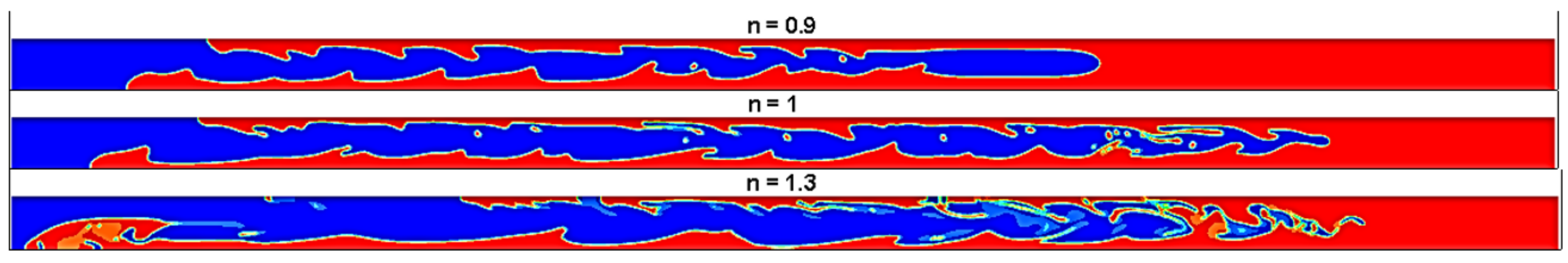
Figure 7,
Figure 8,
Figure 9 and
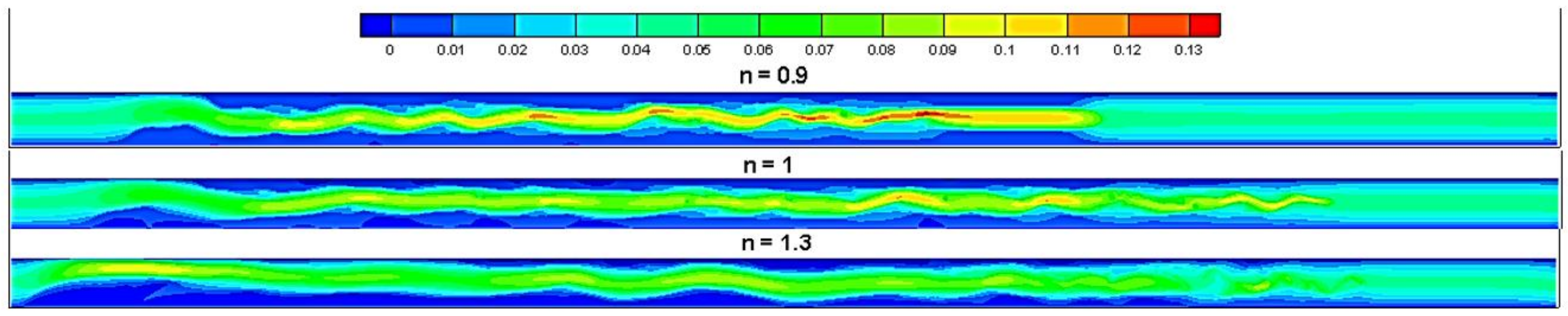
Figure 10 qualitatively show the impacts of the different power-law indices on the flow dynamics, including the density, longitudinal velocity, transverse velocity, and viscosity profile, at
t = 1000
δt.According to the observations shown in
Figure 10, for
, the displaced fluid viscosity has much larger values than those of other displaced materials (i.e., Newtonian and dilatant fluids). This increment in viscous resistive force against injected fluid movement significantly mitigates the total displacement efficiency (
Figure 11). Removing the layers near the channel walls is particularly essential since they are under the severe influence of shear stress.
4.1.1. Displacement Shape Analyses
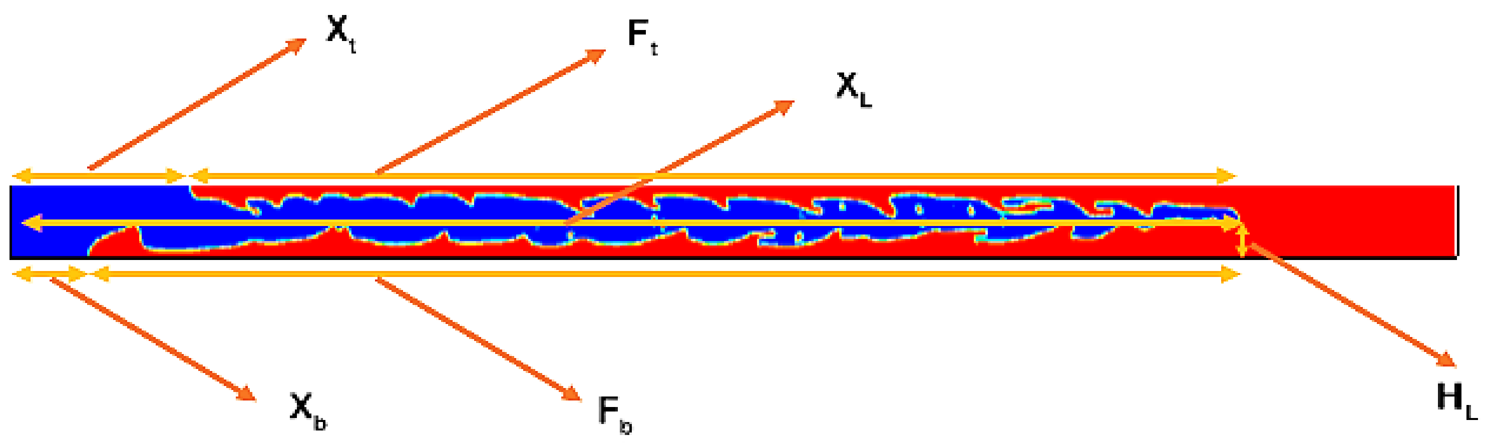
To evaluate the displacement shape in a channel, several measures were defined as shown in
Figure 12; these measures are concisely described in the caption.
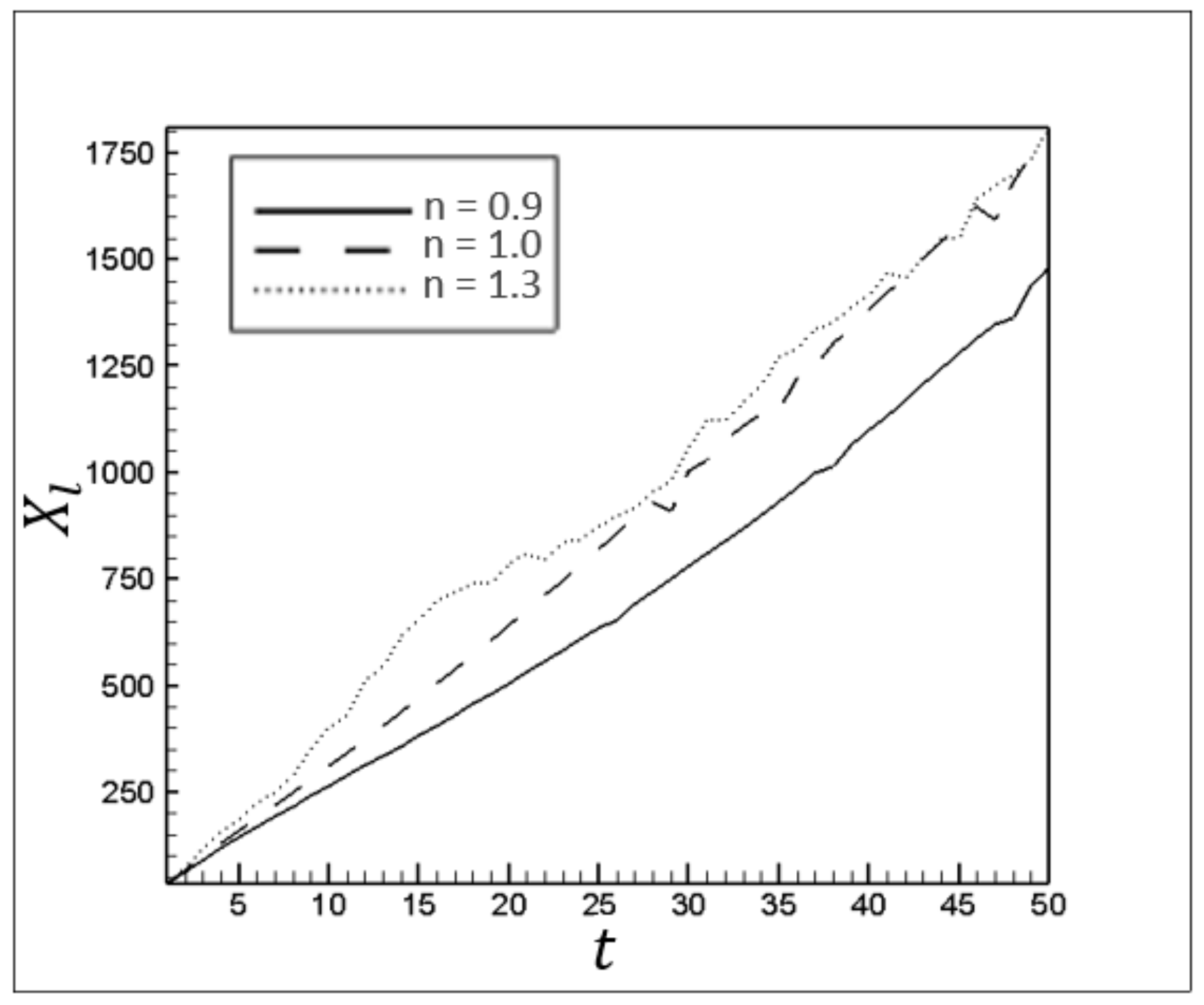
In the case of displacing pseudoplastic materials (
), the maximum value of viscosity, as a function of velocity gradient, occurs near the channel’s central axis. On the contrary, for dilatant fluids (
), the displaced fluid possesses smaller viscosities, and their minimum value occurs near the channel’s central axis. Therefore, the attacking front,
, in the flow with
possesses larger values over time (
Figure 13). This behavior is also repeated for
while
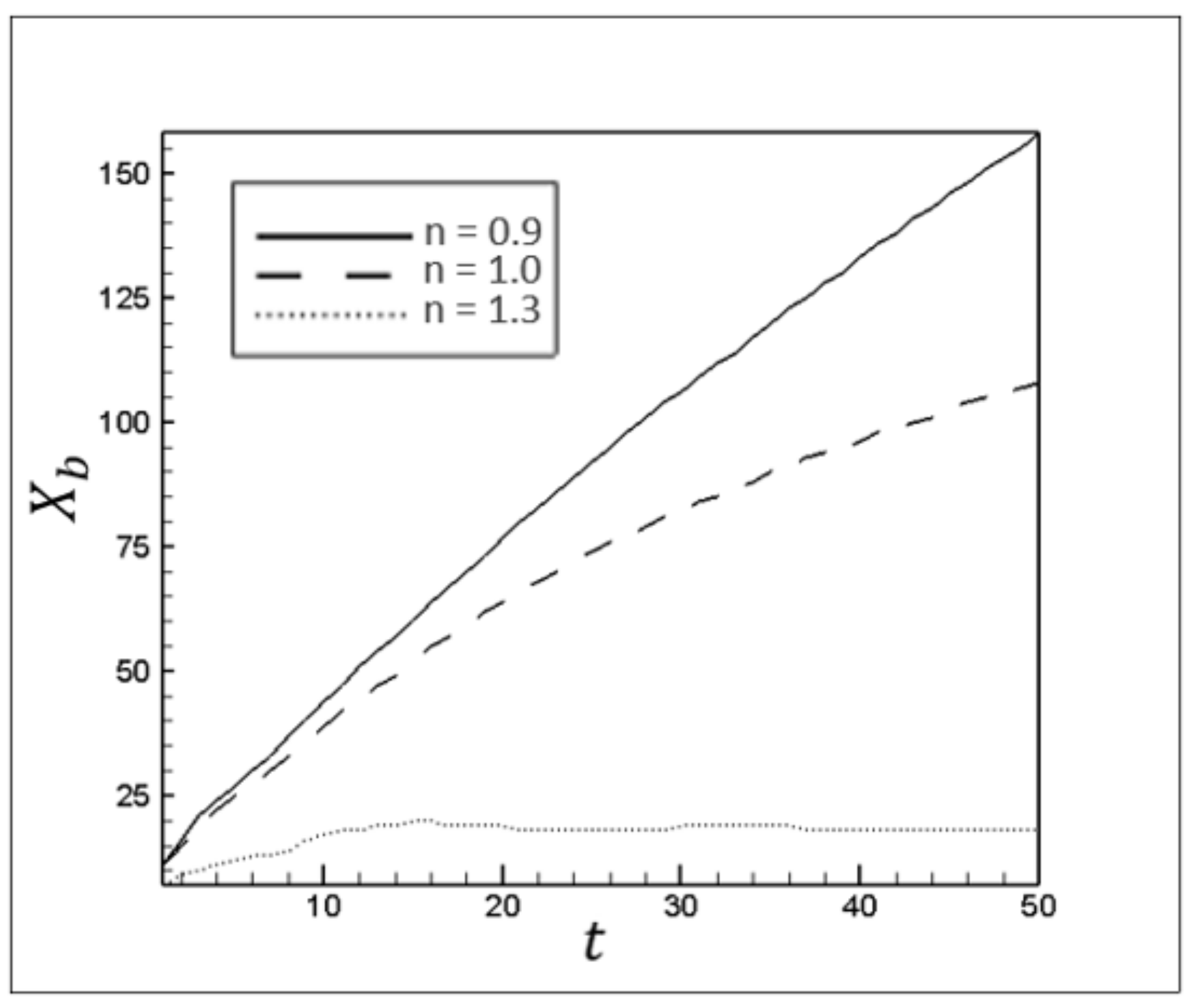
is significantly smaller in value compared to the other displacement flows shown in
Figure 14 and
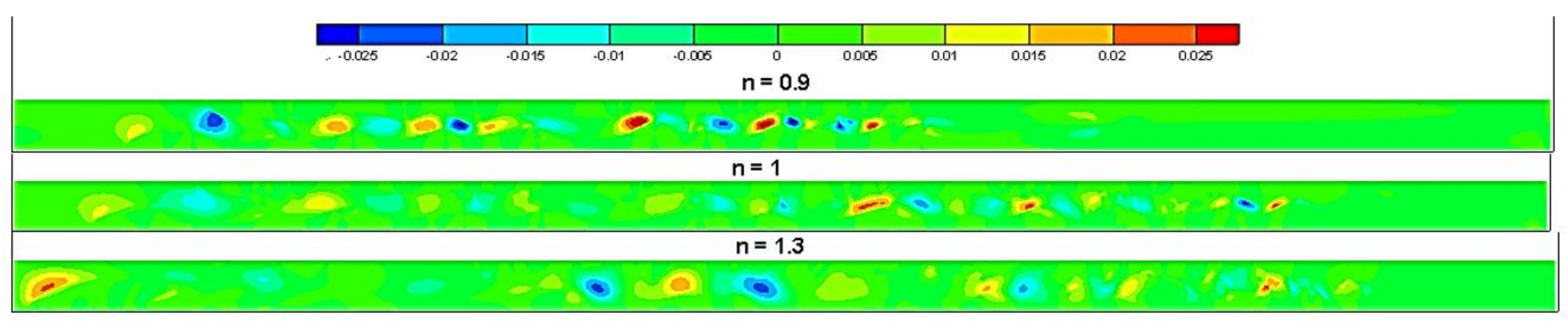
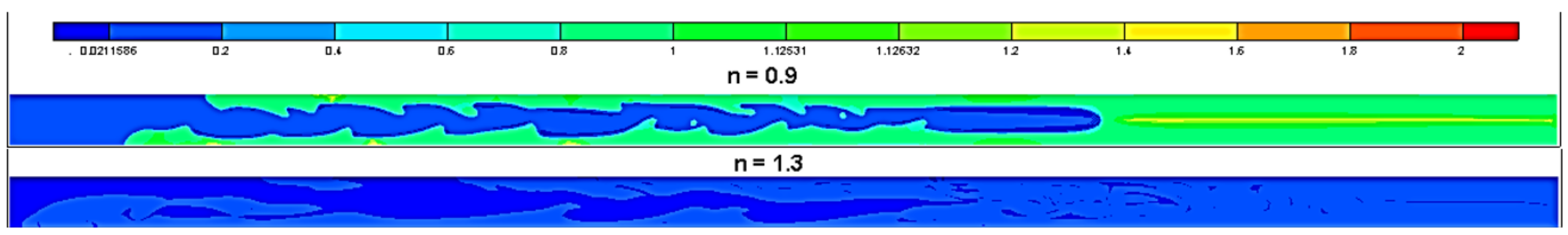
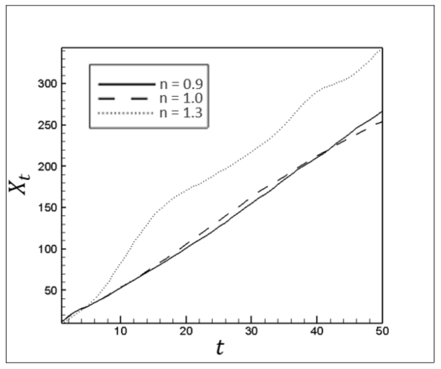
Figure 15. The lower density of the invading fluid due to buoyancy effects and the lower viscosity of the displaced fluid are the main reasons for such behavior. Consequently, the finger structure’s tail tends towards the top of the channel. The development of interfacial instabilities is another contributory factor manipulating injected fluid movement in the channel. In the case of
, the higher viscosity ratio between the fluids considerably mitigated the magnitude of interfacial instabilities (
Figure 7). The stable behavior of the finger structure penetrating in the pseudoplastic fluid (
) counterbalances the impacts of viscous forces on the location of
. Consequently,
shows the same behavior over time in displacing both pseudoplastic and Newtonian fluids.
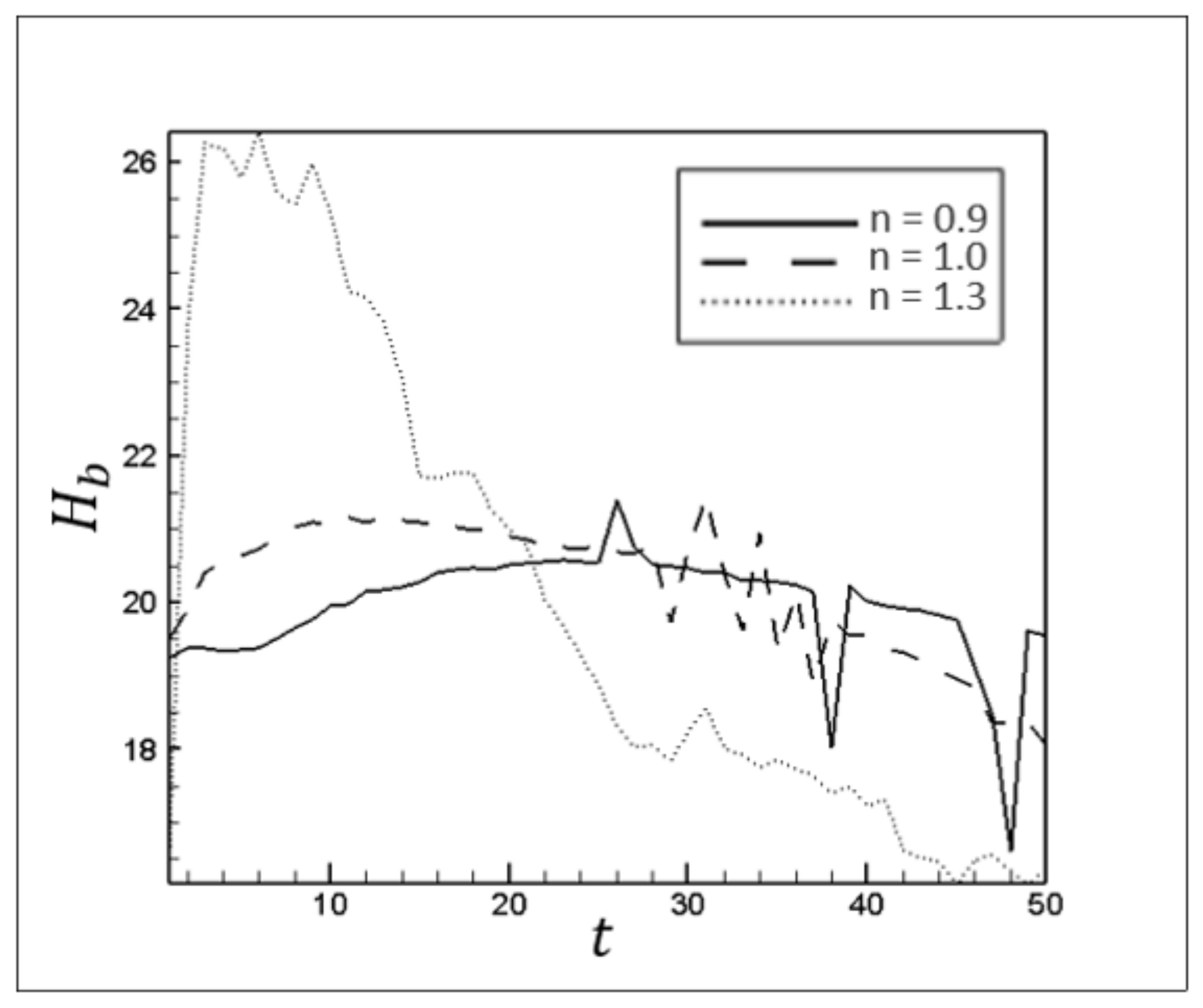
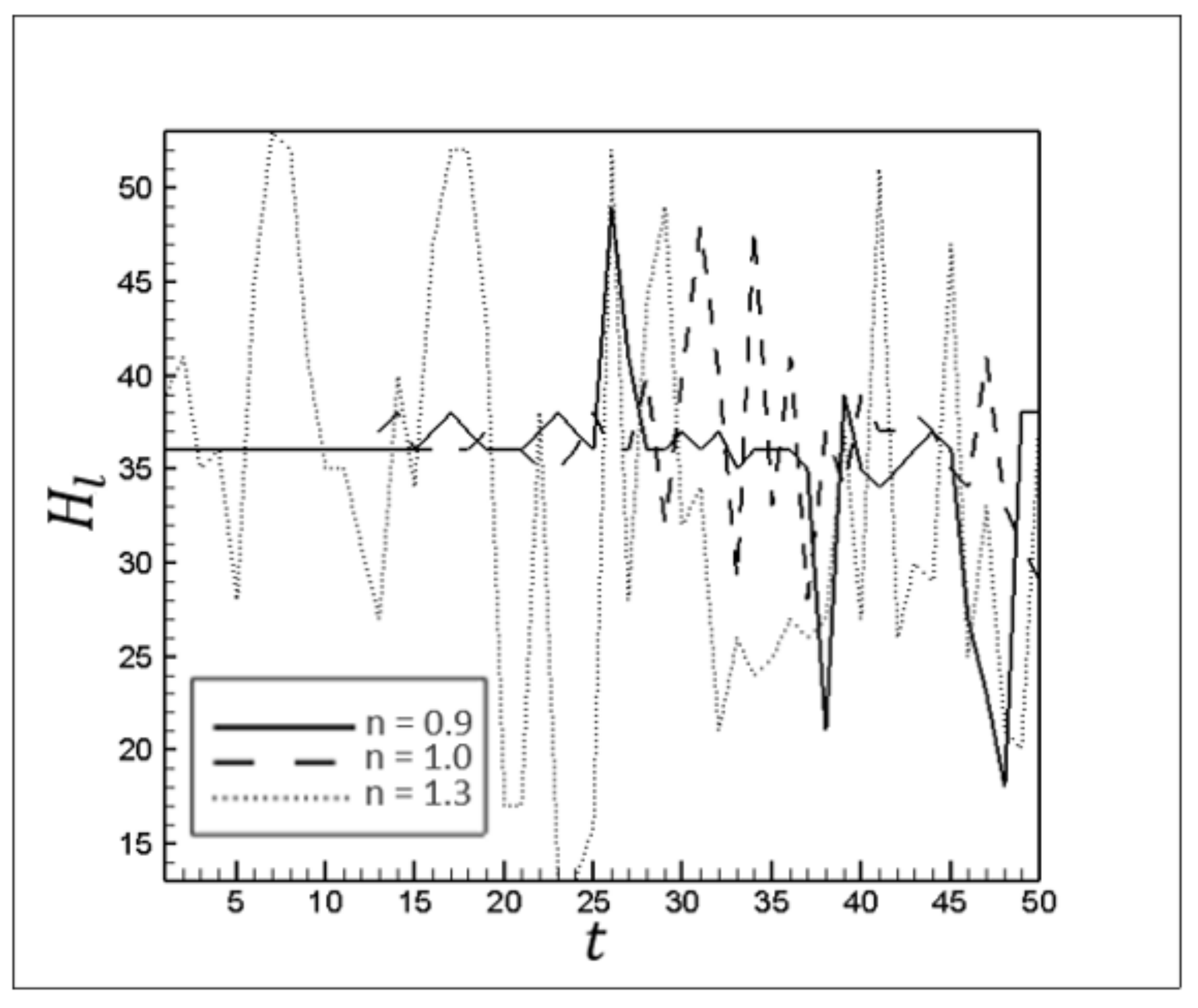
Figure 16 and
Figure 17 show the thickness of the static layers at the top and bottom of the channel,
and
respectively. Since the buoyancy force is a function of the Atwood number, the injected fluid initially experiences the same driving force toward the top wall of the channel for all the cases. Nevertheless, due to the lower viscosity of the displaced fluid with
n = 1.3, a smaller viscous force restricts the upward movement of the injected fluid. In this case, the higher tendency of the injected fluid to move upward is represented by a greater difference between thicknesses of static wall layers adjacent to the channel walls. The viscosity ratio between two fluids at different cross-sections significantly impacts their transverse mixture and penetration. This penetration, along with the transverse velocities (as shown in
Figure 9) and vortices, causes interfacial instabilities and alters the displacement structure. It similarly affects the thickness of the static layer adjacent to the walls. Therefore, in the case of displacing the dilatant fluid (
), enormous fluctuations of the static wall layers attest to the magnification of interfacial instabilities due to the viscosity ratio decrement.
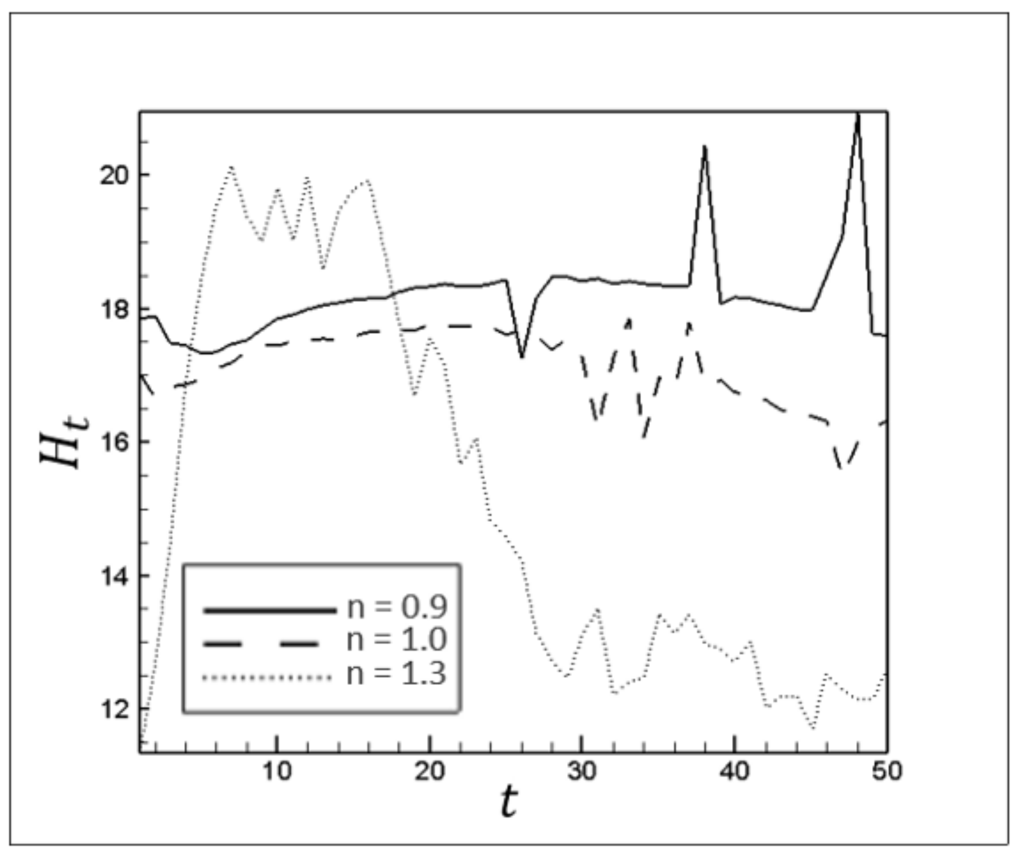
Figure 18 shows the effect of the power-law index on the development of instabilities in terms of transverse fluctuations in the attacking front height,
.
Viscosity ratio and extension of interaction surface between fluids are the two main factors in regulating interfacial instabilities. Increasing the power-law index causes the viscosity of the displaced fluid to approach the viscosity of the invading fluid, which intensifies interfacial instabilities in the finger structure, leading to intense fluctuations in the attacking front height for dilatant fluids.
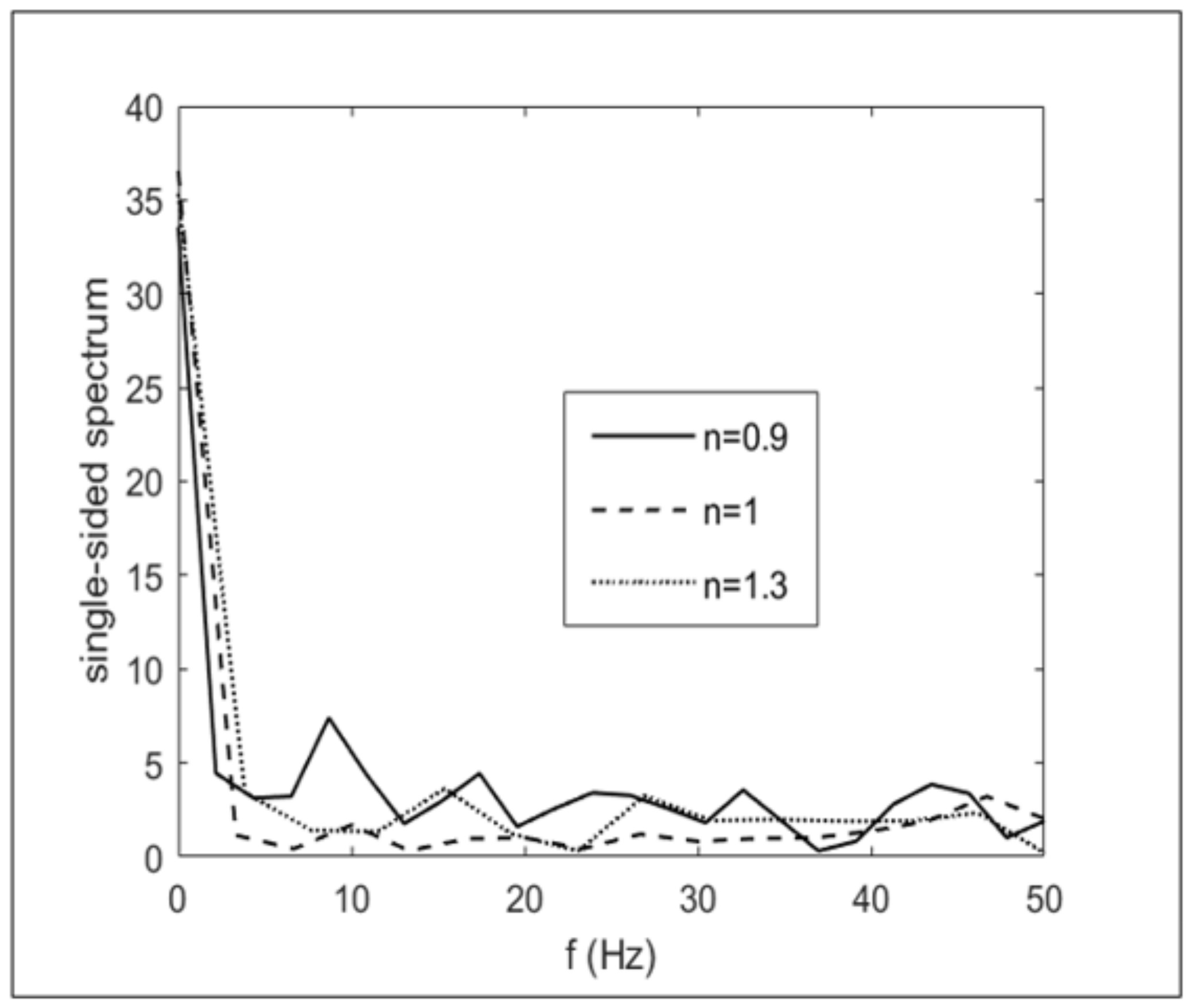
Figure 19 shows the frequency domain analysis of fingertip transverse fluctuations. For this plot, 101 points with a sampling period of 0.5 (dimensionless time) were taken from each line of
Figure 18 to compute the Fourier transform of fluctuations. Subsequently, single-sided spectrums were plotted for each power-law index. Comparing
Figure 18 and
Figure 19 reveals that despite the noisy fluctuations in the fingertip for
n = 0.9, these fluctuations are bigger and more regular when
n = 1.3. Therefore, diminishing the viscous forces promotes the injected fluid’s tendency to move upward and downward regularly.
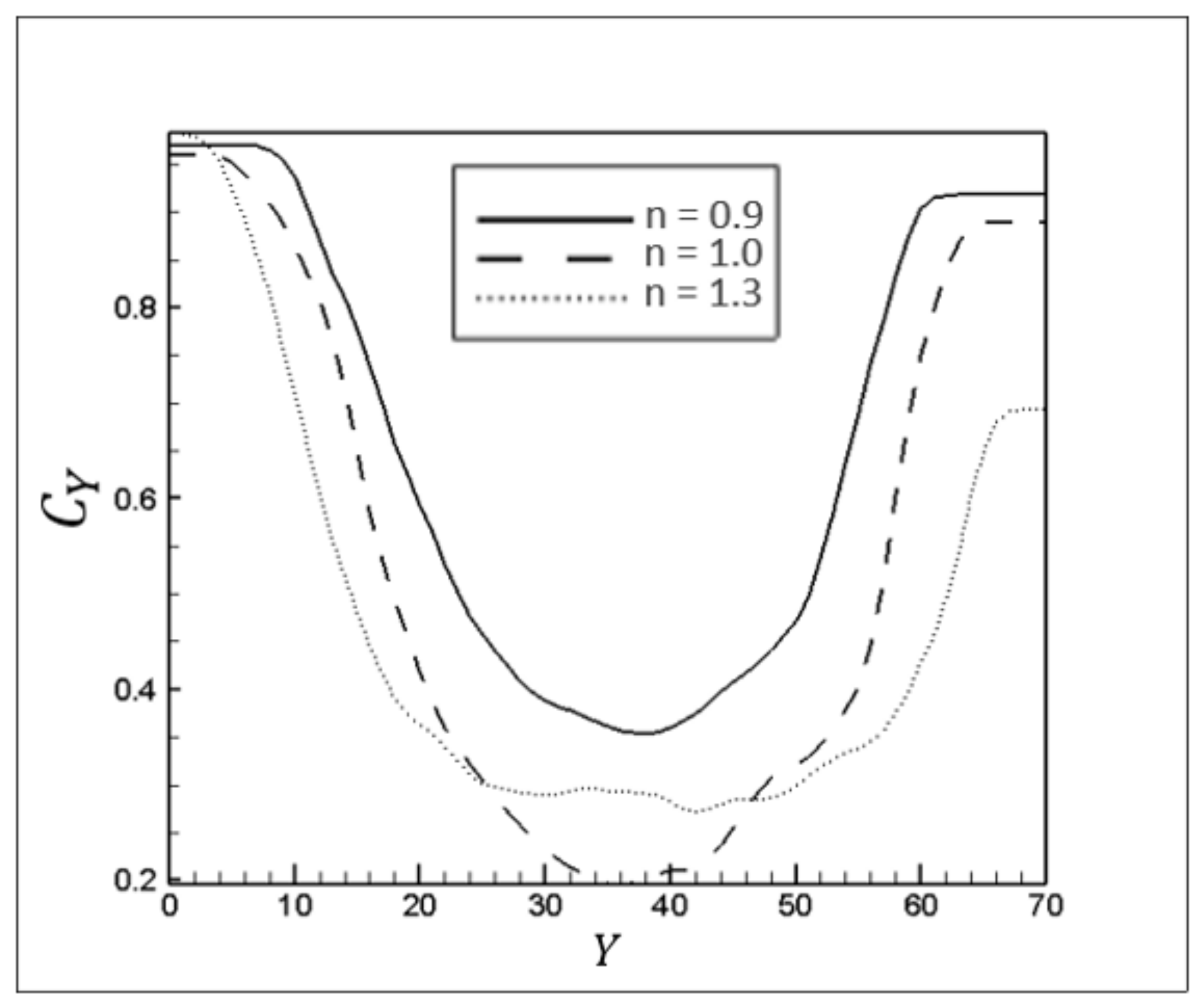
4.1.2. Evaluation of Displacement Efficiency
The advance rate of the injected fluid, the magnitude of interfacial instabilities, and the attacking front fluctuations are evaluated by:
The
and
indices (concentration of displaced fluid) are 1 when the corresponding sections are completely filled by the displaced fluid, and they become 0 when the injected fluid fully displaces the other fluid.
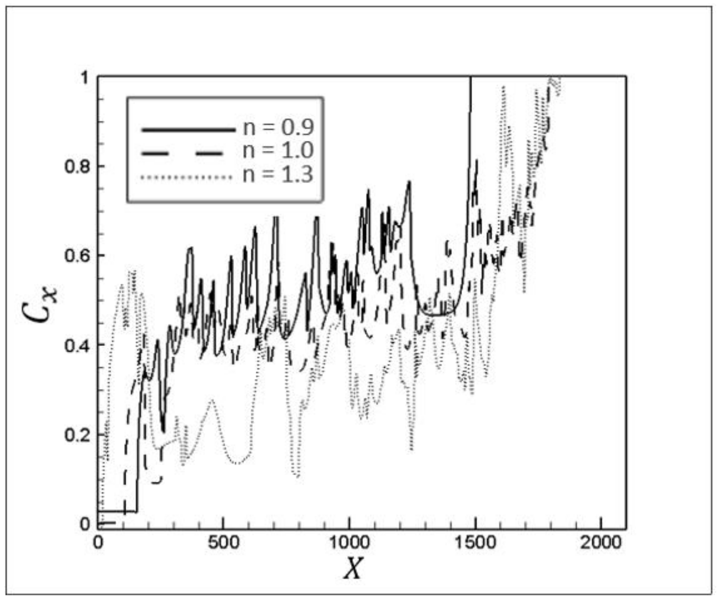
Figure 20 and
Figure 21 present the displacement efficiencies in the longitudinal and transverse axes of the channel. As mentioned before, with the increase of the power-law index, the advance rate of the injected fluid and the displacement efficiency are enhanced in most cross-sections (
Figure 20). Also, severe fluctuations in
show the growth of instabilities with the power-law index enhancement. This trend is repeated for
with the exception that for
, the velocity perturbations in longitudinal sections close to the channel axis are severe enough to considerably influence the displacement efficiency and turn the fingering shape of this curve into a line parallel to the
y-axis.
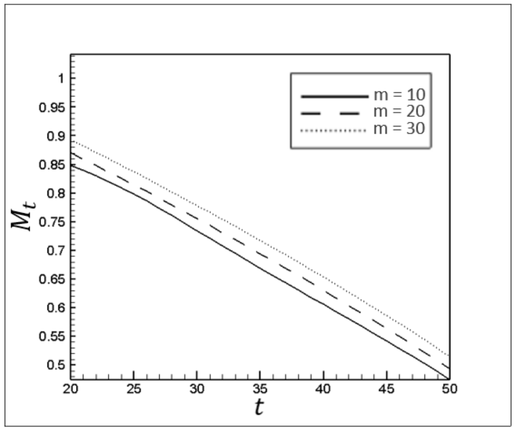
4.2. Impacts of Compatibility Factor
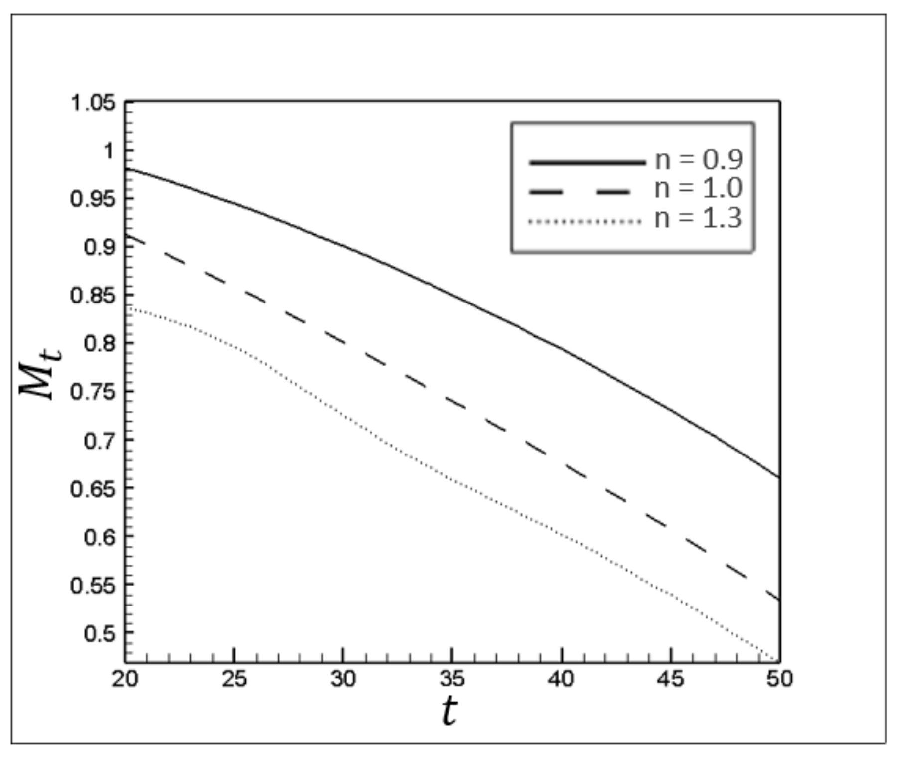
All the simulations in this section were conducted for the power-law index of 1.3. Increasing the displaced fluid’s viscosity through enhancing the compatibility factor reduces the displacement efficiency, as shown in
Figure 22.
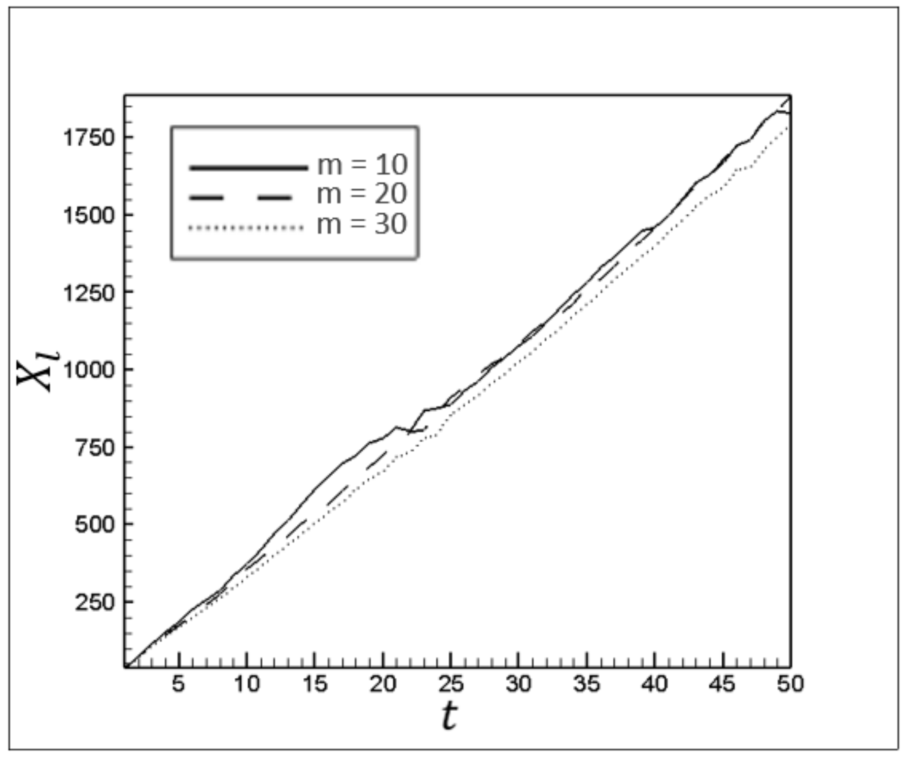
4.2.1. Displacement Shape Analyses
Figure 23,
Figure 24 and
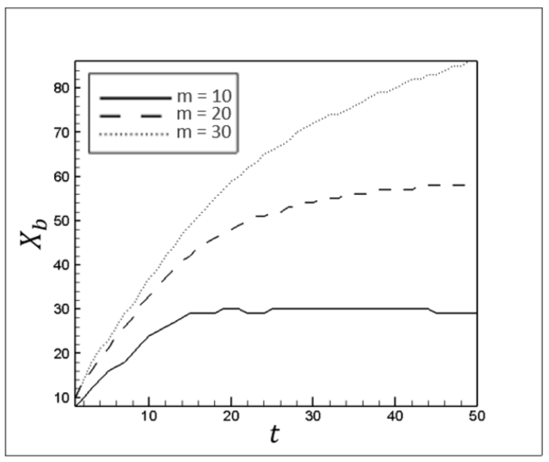
Figure 25 show the effects of the compatibility factor on the velocity of the advancing fronts at the upper part, lower part, and the area between these two sections in the channel. By increasing the viscosity through the compatibility factor growth, the momentum transfer between the fluid’s layers is more severe. This means that displacing static wall layers, which are under the influence of wall shear stress, is more difficult. Therefore, increasing the compatibility factor can magnify the distance between the attacking front and finger structure tails. Nevertheless, given that the injected fluid path is closer to the channel’s upper wall (due to gravitational effects), the attacking front momentum transfers to the tails more severely at the top of the pipe. As a result, by enhancing the viscosity ratio, the distance between the attacking front and lower tail of the finger structure increases, while it has a negligible impact on the upper tail. Moreover, by increasing the viscosity ratio, a more stable flow occurs in which fewer vortices are observed. This provides strong evidence that for lower viscosity ratios, the invading fluid collides with the channel walls.
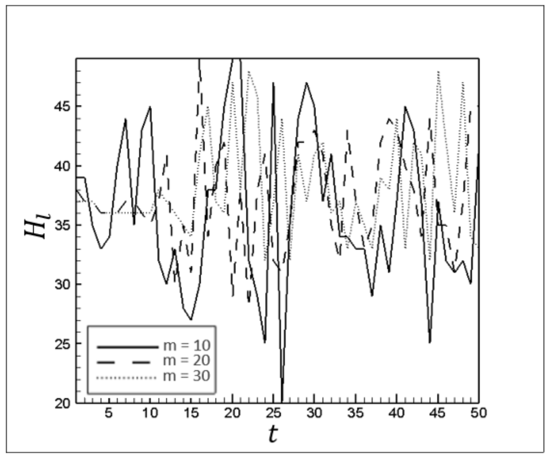
Figure 26 shows the influence of the compatibility factor on the height of the attacking front, which is affected by three primary forces: inertial, viscous, and buoyancy. Because there is little alteration in the buoyancy and inertial forces,
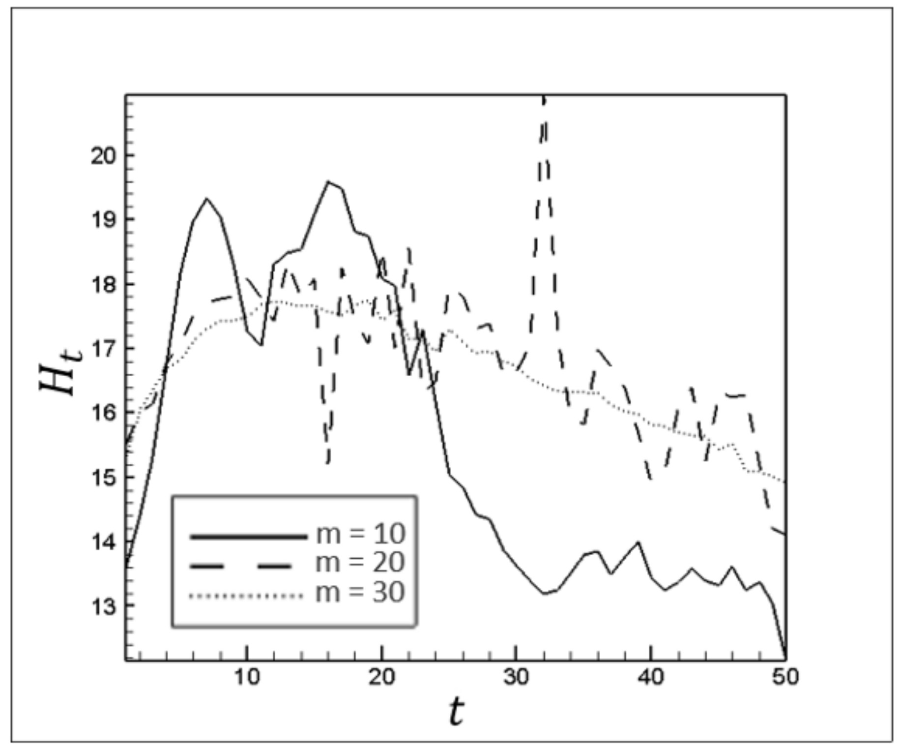
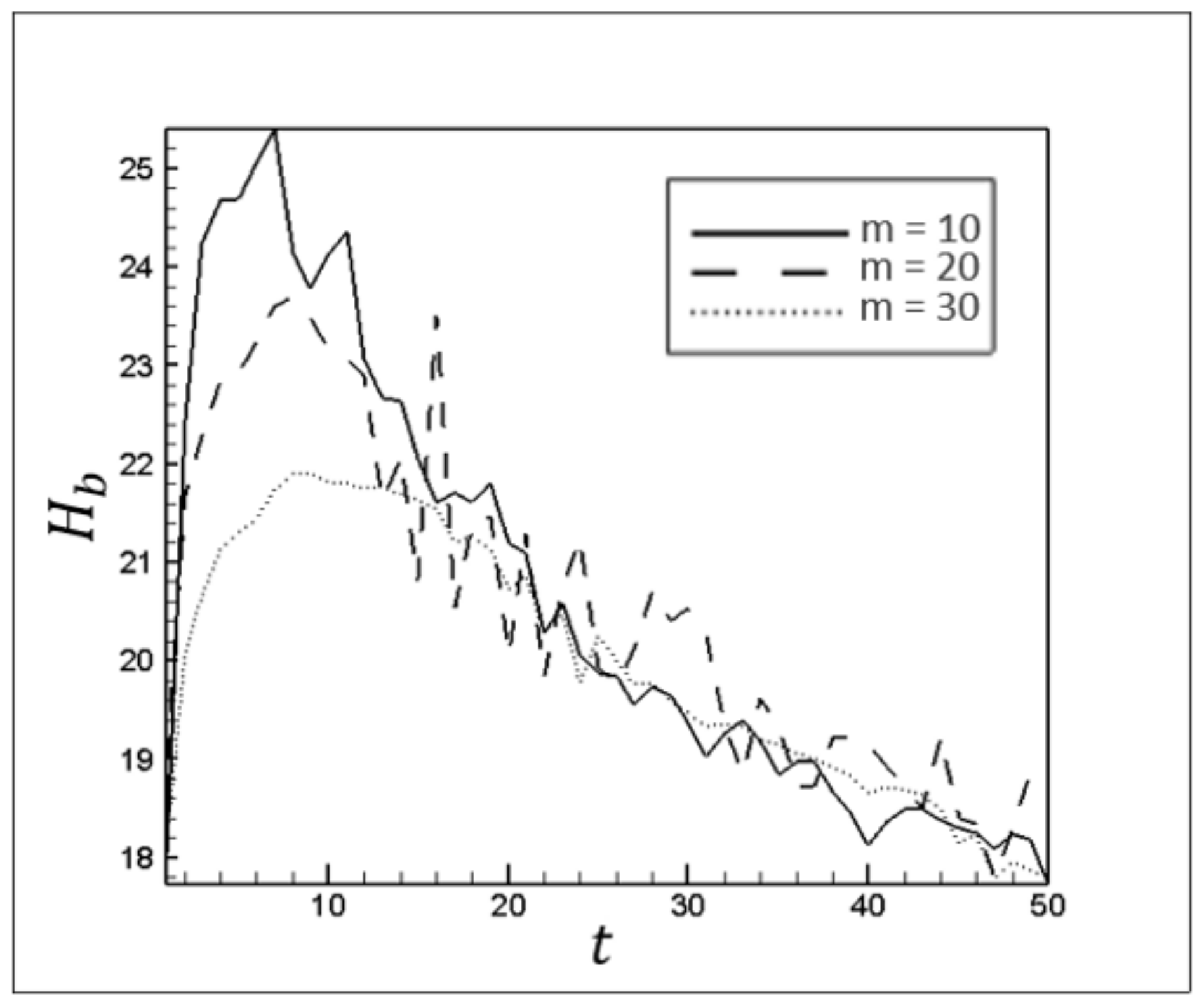
Figure 26 focuses on the effect of viscous force alteration on the attacking front’s perturbation. The impacts of the compatibility factor on the mean thickness of the static layers are illustrated in
Figure 27 and
Figure 28. The changes in the mean thickness of the static layer can be attributed to the generated vortices (as a function of viscosity ratio) and alteration in the injected fluid’s power to transfer the momentum to layers near the channel walls.
4.2.2. Evaluation of Displacement Efficiency
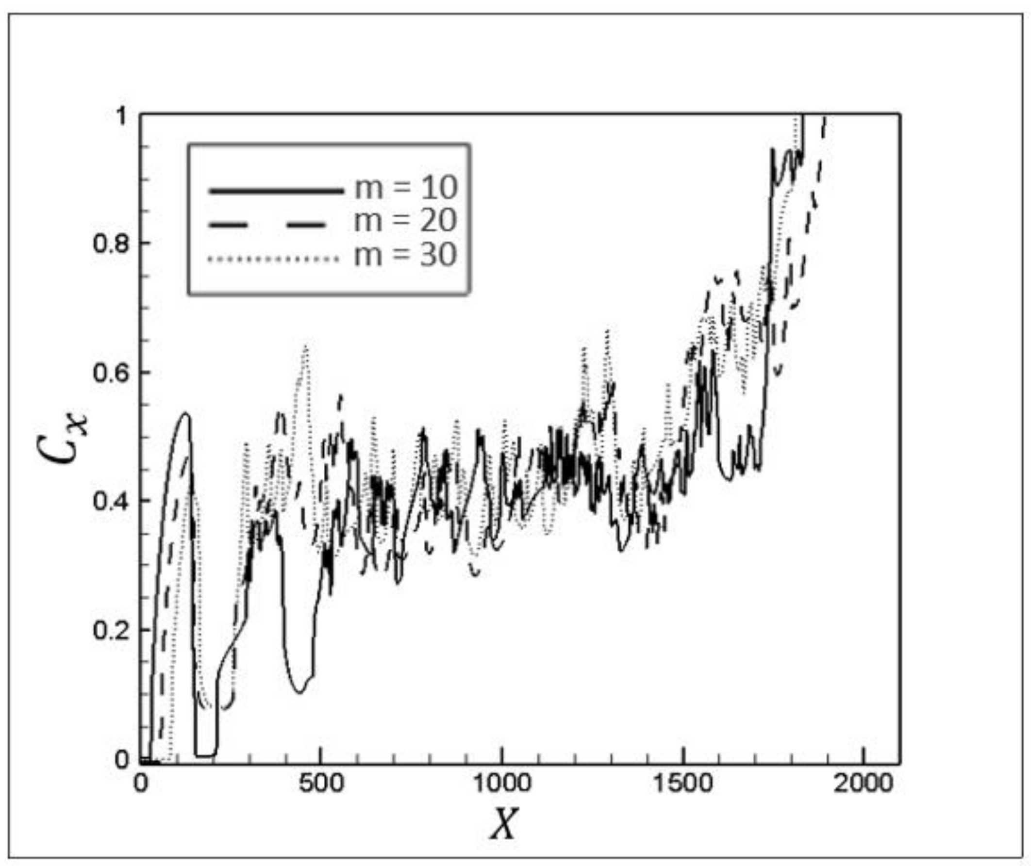
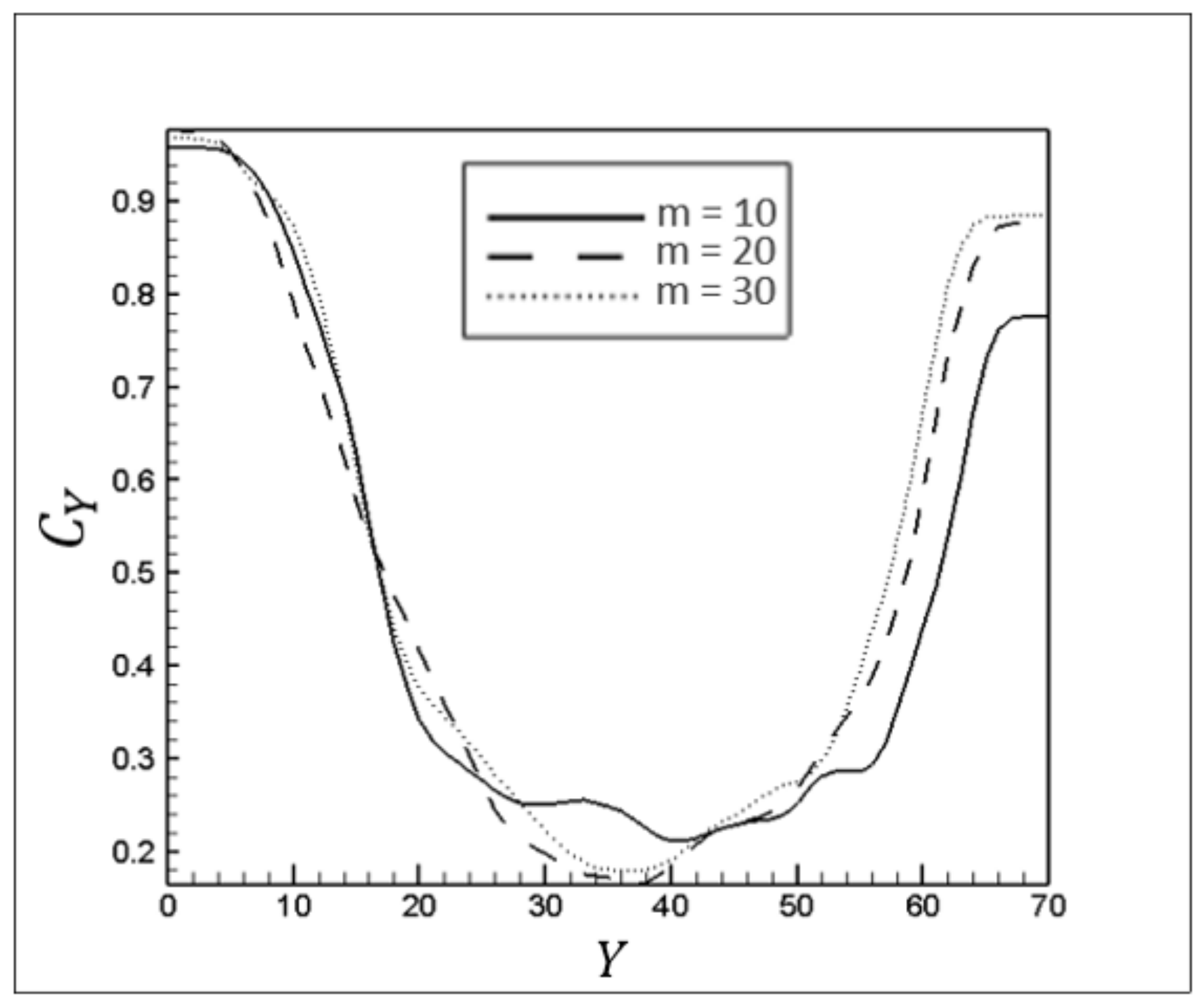
Figure 29 and
Figure 30 show displacement efficiencies in the longitudinal and cross-sectional areas of the pipe for different compatibility factors. Decreasing the viscosity ratio can magnify both Kelvin–Helmholtz and Reighley–Taylor instabilities, which are represented by the high fluctuation of
Cx in
Figure 29. In other words, because of enhanced interfacial instabilities and more severe mixing of the fluids, the mass fraction of the secondary fluid changes more strongly in every cross-section of the channel. It is worth noting that
Cx should fluctuate minimally (in the sections where the fingering structure exists) for a stable penetration with the least perturbations at the fluids’ interface.
5. Discussion
The outcomes of the investigations are discussed below according to the following categories:
Displacement total efficiency: The viscosity ratio can regulate the displacement efficiency in two main ways; firstly, by altering the viscous forces against the invading fluid movement, and secondly, by adjustment of interfacial instabilities. Because of the higher viscosity of pseudoplastic fluids (compared to dilatant materials), it is more difficult for the injected Newtonian fluids to displace them. On the contrary, dilatant materials’ lower viscosity can magnify interfacial instabilities and violate the finger structure’s integrity, leading to higher efficiency. Therefore, the total displacement efficiency is not an appropriate criterion to determine the successful removal of the static wall layer. Consequently, we decided to investigate the displacement efficiency in each longitudinal and cross-sectional area of the channel over time.
Static wall layers: Removing static wall layers is an important issue when dealing with displacement flows and fingering problems. For dilatant materials, the viscous force mitigation against the injected fluid promotes the invading fluid’s tendency to go upward. Therefore, in comparison with other cases, it is expected there will be a thicker wall layer at the bottom of the channel and a thinner one adjacent to the top wall. However, as time elapses, the extension of the finger structure (i.e., interaction surface) magnifies interfacial instabilities. As a result, the static wall layer thickness does not behave according to the expectation for specific periods. In contrast, pseudoplastic fluids possess greater viscosities, and the maximum viscosity takes place around the centerline of the channel. Therefore, the invading fluid tends to move toward the channel walls leading to compression of the static wall layers. This compaction effect causes the static wall layers to initially possess smaller values in displacing pseudoplastic materials.
Finger structure shape: Buoyancy, viscous, and inertial forces control the invasion angle of the finger structure. While the buoyancy force pushes the injected fluid towards the channel walls, the viscous force moderates the finger structure’s upward and downward movement. Accordingly, small fluctuations of the fingertip in displacing pseudoplastic fluids represent the stabilizing effect of the forces. However, due to the low viscosity of dilatant fluids and viscosity ratio, the finger structure looks asymmetric along the longitudinal axis.
Displacing pattern: By tracing the tails of the finger structure, the sweeping power adjacent to the channel walls can be investigated. In pseudoplastic fluids, the higher viscosity of displaced fluid prevents the injected fluid from moving upward. On the other hand, the maximum viscosity of the displaced fluid occurs at the channel centerline, directing the invading fluid toward the channel walls. The two factors counterbalance the effects of each other. As a result, the location of the finger tail at the top of the channel does not change. The higher viscosity of pseudoplastic leads to compaction of the finger structure. Accordingly, the injected fluid tends to completely fill the cross-sectional areas at the beginning of the channel and move ahead. However, the injected fluid tends to reach the end of the channel rather than filling the cross-sectional areas when a Newtonian fluid is injected to displace a dilatant fluid.
Compatibility factor vs. power-law index: There is a linear relationship between viscosity and the compatibility factor. As expected, increasing the compatibility factor of the displaced fluid results in a reduction in displacement efficiency. However, compared to the nonlinear impact of the power-law index, compatibility factor alteration has a negligible effect on the location of the fingertip and top tail.
6. Conclusions
In this study, a multi-component model of the lattice Boltzmann method, called the He–Chen–Zhang model, was used to simulate the pressure-driven displacement of non-Newtonian fluid (power-law) by Newtonian fluids in 2D inclined channels. Based on this approach and 9-speed square lattices, a multi-purpose code was developed in this study that enabled us to carry out simulations with high viscosity ratios. Several simulations were conducted to evaluate the impacts of viscosity determination criteria on flow pattern, the development of interfacial instabilities, and sectional efficiency of displacement flow.
It was demonstrated that the fingertip structure is enforced by the interaction of buoyancy, viscous, and inertial forces while it is stabilized by the growth of the viscosity ratio in pseudoplastic fluids. It was found that the viscosity ratio can regulate the displacement efficiency while the total displacement efficiency is not an appropriate criterion to assess the successful removal of static wall layers. Furthermore, the thickness of static wall layers at the top and the bottom of the channel, due to interfacial instabilities, dynamically changes over time. As a result, the injected fluid tends to completely fill the cross-sectional areas at the beginning of the channel and move ahead for pseudoplastic fluids, while the injected fluid tends to reach the end of the channel rather than filling the cross-sectional areas in the case of dilatant fluids. In addition, increasing the compatibility factor of the displaced fluid linearly reduces the displacement efficiencies, and it has negligible impact on the finger structure.
Enhancement of immiscible two-phase displacement flows in industrial applications requires a deep understanding of fluid’s behavior and implementing innovative approaches to control fluid motion in the desired direction. This study and another research project regarding the impact of electro-and magneto-hydrodynamics on the fingering pattern [
8] were devised to improve the performance of displacement flows. Investigation of the near-interface dissociation-recombination layers and EHD conduction pumping inside non-Newtonian material is an interesting topic that would be another step forward in this direction.
Author Contributions
Conceptualization, M.E.; Investigation, M.E. and M.G.K.; Methodology, M.E.; Project administration, M.E.; Software, M.E.; Supervision, M.G.K.; Validation, M.E.; Visualization, M.E.; Writing—original draft, M.E.; Writing—review & editing, M.G.K. All authors have read and agreed to the published version of the manuscript.
Funding
The APC was funded by the KIT Publication Fund of the Karlsruhe Institute of Technology.
Data Availability Statement
The data that support the findings of this study are available from the corresponding author upon reasonable request.
Acknowledgments
The study is part of the Helmholtz portfolio project “Geoenergy”. The support from the program, “Renewable Energies”, under the topic “Geothermal Energy Systems”, is gratefully acknowledged. Moreover, we acknowledge the support provided by the KIT Publication Fund of the Karlsruhe Institute of Technology.
Conflicts of Interest
The authors declare no conflict of interest.
References
- Muggeridge, A.; Cockin, A.; Webb, K.; Frampton, H.; Collins, I.; Moulds, T.; Salino, P. Recovery rates, enhanced oil recovery and technological limits. Philos. Trans. R. Soc. A Math. Phys. Eng. Sci. 2014, 372, 20120320. [Google Scholar] [CrossRef]
- Kargozarfard, Z.; Riazi, M.; Ayatollahi, S. Viscous fingering and its effect on areal sweep efficiency during waterflooding: An experimental study. Pet. Sci. 2019, 16, 105–116. [Google Scholar] [CrossRef]
- Suzuki, R.X.; Nagatsu, Y.; Mishra, M.; Ban, T. Phase separation effects on a partially miscible viscous fingering dynamics. J. Fluid Mech. 2020, 898, A11. [Google Scholar] [CrossRef]
- Song, W.; Ramesh, N.N.; Kovscek, A.R. Spontaneous fingering between miscible fluids. Colloids Surfaces A Physicochem. Eng. Asp. 2020, 584, 123943. [Google Scholar] [CrossRef]
- Abdul Hamid, S.A.; Muggeridge, A.H. Fingering regimes in unstable miscible displacements. Phys. Fluids 2020, 32, 016601. [Google Scholar] [CrossRef]
- Tsuzuki, R.; Ban, T.; Fujimura, M.; Nagatsu, Y. Dual role of surfactant-producing reaction in immiscible viscous fingering evolution. Phys. Fluids 2019, 31, 022102. [Google Scholar] [CrossRef]
- Jackson, S.J.; Power, H.; Giddings, D. Immiscible thermo-viscous fingering in Hele-Shaw cells. Comput. Fluids 2017, 156, 621–641. [Google Scholar] [CrossRef][Green Version]
- Esmaeilpour, M.; Gholami Korzani, M. Enhancement of immiscible two-phase displacement flow by introducing nanoparticles and employing electro- and magneto-hydrodynamics. J. Pet. Sci. Eng. 2021, 196, 108044. [Google Scholar] [CrossRef]
- Goyal, N.; Meiburg, E. Miscible displacements in Hele-Shaw cells: Two-dimensional base states and their linear stability. J. Fluid Mech. 2006, 558, 329. [Google Scholar] [CrossRef]
- Petitjeans, P.; Maxworthy, T. Miscible displacements in capillary tubes. Part 1. Experiments. J. Fluid Mech. 1996, 326, 37–56. [Google Scholar] [CrossRef]
- Lajeunesse, E.; Martin, J.; Rakotomalala, N.; Salin, D.; Yortsos, Y.C. Miscible displacement in a Hele-Shaw cell at high rates. J. Fluid Mech. 1999, 398, 299–319. [Google Scholar] [CrossRef]
- Taghavi, S.M.; Séon, T.; Wielage-Burchard, K.; Martinez, D.M.; Frigaard, I.A. Stationary residual layers in buoyant Newtonian displacement flows. Phys. Fluids 2011, 23, 044105. [Google Scholar] [CrossRef]
- Taghavi, S.M.; Seon, T.; Martinez, D.M.; Frigaard, I.A. Buoyancy-dominated displacement flows in near-horizontal channels: The viscous limit. J. Fluid Mech. 2009, 639, 1–35. [Google Scholar] [CrossRef]
- Sahu, K.C.; Ding, H.; Valluri, P.; Matar, O.K. Pressure-driven miscible two-fluid channel flow with density gradients. Phys. Fluids 2009, 21, 043603. [Google Scholar] [CrossRef]
- Sahu, K.C.; Ding, H.; Valluri, P.; Matar, O.K. Linear stability analysis and numerical simulation of miscible two-layer channel flow. Phys. Fluids 2009, 21, 042104. [Google Scholar] [CrossRef]
- Yang, Z.; Yortsos, Y.C. Asymptotic solutions of miscible displacements in geometries of large aspect ratio. Phys. Fluids 1997, 9, 286–298. [Google Scholar] [CrossRef]
- Bischofberger, I.; Ramachandran, R.; Nagel, S.R. Fingering versus stability in the limit of zero interfacial tension. Nat. Commun. 2014, 5, 5265. [Google Scholar] [CrossRef]
- Shabouei, M.; Nakshatrala, K.B. On Numerical Stabilization in Modeling Double-Diffusive Viscous Fingering. Transp. Porous Media 2020, 132, 39–52. [Google Scholar] [CrossRef]
- Redapangu, P.R.; Chandra Sahu, K.; Vanka, S.P. A study of pressure-driven displacement flow of two immiscible liquids using a multiphase lattice Boltzmann approach. Phys. Fluids 2012, 24, 102110. [Google Scholar] [CrossRef]
- Dimakopoulos, Y.; Tsamopoulos, J. Transient displacement of a viscoplastic material by air in straight and suddenly constricted tubes. J. Nonnewton. Fluid Mech. 2003, 112, 43–75. [Google Scholar] [CrossRef]
- Papaioannou, J.; Karapetsas, G.; Dimakopoulos, Y.; Tsamopoulos, J. Injection of a viscoplastic material inside a tube or between two parallel disks: Conditions for wall detachment of the advancing front. J. Rheol. 2009, 53, 1155–1191. [Google Scholar] [CrossRef]
- Ebrahimi, B.; Mostaghimi, P.; Gholamian, H.; Sadeghy, K. Viscous fingering in yield stress fluids: A numerical study. J. Eng. Math. 2016, 97, 161–176. [Google Scholar] [CrossRef]
- Wielage-Burchard, K.; Frigaard, I.A. Static wall layers in plane channel displacement flows. J. Nonnewton. Fluid Mech. 2011, 166, 245–261. [Google Scholar] [CrossRef]
- Frigaard, I.A.; Nouar, C. On the usage of viscosity regularisation methods for visco-plastic fluid flow computation. J. Nonnewton. Fluid Mech. 2005, 127, 1–26. [Google Scholar] [CrossRef]
- Allouche, M.; Frigaard, I.A.; Sona, G. Static wall layers in the displacement of two visco-plastic fluids in a plane channel. J. Fluid Mech. 2000, 424, 243–277. [Google Scholar] [CrossRef]
- Mitsoulis, E.; Tsamopoulos, J. Numerical simulations of complex yield-stress fluid flows. Rheol. Acta 2017, 56, 231–258. [Google Scholar] [CrossRef]
- Khan, N.A.; Sultan, F. Numerical Analysis for the Bingham—Papanastasiou Fluid Flow Over a Rotating Disk. J. Appl. Mech. Tech. Phys. 2018, 59, 638–644. [Google Scholar] [CrossRef]
- Baakeem, S.S.; Bawazeer, S.A.; Mohamad, A.A. Comparison and evaluation of Shan–Chen model and most commonly used equations of state in multiphase lattice Boltzmann method. Int. J. Multiph. Flow 2020, 128, 103290. [Google Scholar] [CrossRef]
- Chen, N.; Jin, Z.; Liu, Y.; Wang, P.; Chen, X. Lattice Boltzmann simulations of droplet dynamics in two-phase separation with temperature field. Phys. Fluids 2020, 32, 073312. [Google Scholar] [CrossRef]
- Gholami Korzani, M.; Galindo-Torres, S.A.; Scheuermann, A.; Williams, D.J. Smoothed Particle Hydrodynamics for investigating hydraulic and mechanical behaviour of an embankment under action of flooding and overburden loads. Comput. Geotech. 2018, 94, 31–45. [Google Scholar] [CrossRef]
- Gholami Korzani, M.; Galindo Torres, S.; Scheuermann, A.; Williams, D.J. Smoothed Particle Hydrodynamics into the Fluid Dynamics of Classical Problems. Appl. Mech. Mater. 2016, 846, 73–78. [Google Scholar] [CrossRef]
- Gholami Korzani, M.; Galindo-Torres, S.A.; Williams, D.; Scheuermann, A. Numerical Simulation of Tank Discharge Using Smoothed Particle Hydrodynamics. Appl. Mech. Mater. 2014, 553, 168–173. [Google Scholar] [CrossRef]
- Esmaeilpour, M.; Gholami Korzani, M.; Kohl, T. Performance Analyses of Deep Closed-loop U-shaped Heat Exchanger System with a Long Horizontal Extension. In Proceedings of the 46th Workshop on Geothermal Reservoir Engineering, Stanford, CA, USA, 16–18 February 2021; Stanford University: Stanford, CA, USA, 2021. [Google Scholar]
- Sudhakar, T.; Das, A.K. Evolution of Multiphase Lattice Boltzmann Method: A Review. J. Inst. Eng. Ser. C 2020, 101, 711–719. [Google Scholar] [CrossRef]
- He, X.; Chen, S.; Zhang, R. A Lattice Boltzmann Scheme for Incompressible Multiphase Flow and Its Application in Simulation of Rayleigh–Taylor Instability. J. Comput. Phys. 1999, 152, 642–663. [Google Scholar] [CrossRef]
- He, X.; Zhang, R.; Chen, S.; Doolen, G.D. On the three-dimensional Rayleigh–Taylor instability. Phys. Fluids 1999, 11, 1143–1152. [Google Scholar] [CrossRef]
- Sahu, K.C.; Vanka, S.P. A multiphase lattice Boltzmann study of buoyancy-induced mixing in a tilted channel. Comput. Fluids 2011, 50, 199–215. [Google Scholar] [CrossRef]
- Ezzatneshan, E.; Vaseghnia, H. Evaluation of equations of state in multiphase lattice Boltzmann method with considering surface wettability effects. Phys. A Stat. Mech. Its Appl. 2020, 541, 123258. [Google Scholar] [CrossRef]
- Ishak, M.H.H.; Ismail, F.; Abdul Aziz, M.S.; Abdullah, M.Z. Effect of adhesive force on underfill process based on lattice Boltzmann method. Microelectron. Int. 2020, 37, 54–63. [Google Scholar] [CrossRef]
- Yuana, K.A.; Budiana, E.P.; Deendarlianto; Indarto. Modeling and simulation of droplet wettability using multiphase Lattice Boltzmann method (LBM). AIP Conf. Proc. 2019, 2192, 070002. [Google Scholar]
- Zachariah, G.T.; Panda, D.; Surasani, V.K. Lattice Boltzmann simulations for invasion patterns during drying of capillary porous media. Chem. Eng. Sci. 2019, 196, 310–323. [Google Scholar] [CrossRef]
- Yang, L.; Yu, Y.; Yang, L.; Hou, G. Analysis and assessment of the no-slip and slip boundary conditions for the discrete unified gas kinetic scheme. Phys. Rev. E 2020, 101, 023312. [Google Scholar] [CrossRef]
- Noble, D.R.; Georgiadis, J.G.; Buckius, R.O. Direct assessment of lattice Boltzmann hydrodynamics and boundary conditions for recirculating flows. J. Stat. Phys. 1995, 81, 17–33. [Google Scholar] [CrossRef]
- Guo, Z.; Zheng, C.; Shi, B. An extrapolation method for boundary conditions in lattice Boltzmann method. Phys. Fluids 2002, 14, 2007–2010. [Google Scholar] [CrossRef]
- Chen, S.; Martínez, D.; Mei, R. On boundary conditions in lattice Boltzmann methods. Phys. Fluids 1996, 8, 2527–2536. [Google Scholar] [CrossRef]
- Zhao-Li, G.; Chu-Guang, Z.; Bao-Chang, S. Non-equilibrium extrapolation method for velocity and pressure boundary conditions in the lattice Boltzmann method. Chin. Phys. B 2002, 11, 366. [Google Scholar] [CrossRef]
- Amani, A.; Balcázar, N.; Naseri, A.; Rigola, J. A numerical approach for non-Newtonian two-phase flows using a conservative level-set method. Chem. Eng. J. 2020, 385, 123896. [Google Scholar] [CrossRef]
- Ionescu, C.M.; Birs, I.R.; Copot, D.; Muresan, C.I.; Caponetto, R. Mathematical modelling with experimental validation of viscoelastic properties in non-Newtonian fluids. Philos. Trans. R. Soc. A Math. Phys. Eng. Sci. 2020, 378, 20190284. [Google Scholar] [CrossRef] [PubMed]
- Shende, T.; Niasar, V.J.; Babaei, M. Effective viscosity and Reynolds number of non-Newtonian fluids using Meter model. Rheol. Acta 2021, 60, 11–21. [Google Scholar] [CrossRef]
- Lin, Y.; Yang, M. Marangoni flow and mass transfer of power-law non-Newtonian fluids over a disk with suction and injection. Commun. Theor. Phys. 2020, 72, 095003. [Google Scholar] [CrossRef]
- Yazdani, K.; Sahebjamei, M.; Ahmadpour, A. Natural Convection Heat Transfer and Entropy Generation in a Porous Trapezoidal Enclosure Saturated with Power-Law Non-Newtonian Fluids. Heat Transf. Eng. 2020, 41, 982–1001. [Google Scholar] [CrossRef]
- Battistella, A.; van Schijndel, S.J.G.; Baltussen, M.W.; Roghair, I.; van Sint Annaland, M. On the terminal velocity of single bubbles rising in non-Newtonian power-law liquids. J. Nonnewton. Fluid Mech. 2020, 278, 104249. [Google Scholar] [CrossRef]
Figure 1.
A schematic illustration of the geometrical configuration (not to scale) and initial flow structure.
Figure 1.
A schematic illustration of the geometrical configuration (not to scale) and initial flow structure.
Figure 2.
Stress changes versus shear rates in power-law fluids for different n ( = 0.4).
Figure 2.
Stress changes versus shear rates in power-law fluids for different n ( = 0.4).
Figure 3.
Viscosity changes versus shear rates in power-law fluids for different n ( = 0.4).
Figure 3.
Viscosity changes versus shear rates in power-law fluids for different n ( = 0.4).
Figure 4.
A comparison between the results of the present study and Redapangu et al. [
19].
Figure 4.
A comparison between the results of the present study and Redapangu et al. [
19].
Figure 5.
The effects of changes in the lattice layout on changes in at different times.
Figure 5.
The effects of changes in the lattice layout on changes in at different times.
Figure 6.
The effects of changes in the lattice layout on the mean thickness of the static layer left on the lower wall of the channel at different times.
Figure 6.
The effects of changes in the lattice layout on the mean thickness of the static layer left on the lower wall of the channel at different times.
Figure 7.
The apparent shape of the finger structure for different n.
Figure 7.
The apparent shape of the finger structure for different n.
Figure 8.
The longitudinal velocity of the mixture for different n.
Figure 8.
The longitudinal velocity of the mixture for different n.
Figure 9.
The transverse velocity of the mixture for different n.
Figure 9.
The transverse velocity of the mixture for different n.
Figure 10.
The viscosity contour for different n.
Figure 10.
The viscosity contour for different n.
Figure 11.
Displacement efficiency versus time for different n.
Figure 11.
Displacement efficiency versus time for different n.
Figure 12.
A schematic demonstration of the displacement shape. is the location of the invading fluid front at the top of the channel, and is a similar location at the bottom of the channel. is called the attacking front, which is the front of the finger-like structure in the longitudinal direction. and represent the length of the finger structure (). is the height of the attacking front.
Figure 13.
The attacking front location, , over time for different n.
Figure 13.
The attacking front location, , over time for different n.
Figure 14.
The invading fluid front at the top of the channel, , over time for different n.
Figure 14.
The invading fluid front at the top of the channel, , over time for different n.
Figure 15.
The invading fluid front at the bottom of the channel, , over time for different n.
Figure 15.
The invading fluid front at the bottom of the channel, , over time for different n.
Figure 16.
The mean thickness of the static layer at the top of the channel, , over time for different n.
Figure 16.
The mean thickness of the static layer at the top of the channel, , over time for different n.
Figure 17.
The mean thickness of the static layer at the bottom of the channel, , over time for different n.
Figure 17.
The mean thickness of the static layer at the bottom of the channel, , over time for different n.
Figure 18.
The attacking front height, , over time for different n.
Figure 18.
The attacking front height, , over time for different n.
Figure 19.
Frequency domains of fingertip transverse fluctuations for different n.
Figure 19.
Frequency domains of fingertip transverse fluctuations for different n.
Figure 20.
Transverse displacement efficiency over the channel length for different n.
Figure 20.
Transverse displacement efficiency over the channel length for different n.
Figure 21.
Longitudinal displacement efficiency over the channel height for different n.
Figure 21.
Longitudinal displacement efficiency over the channel height for different n.
Figure 22.
Displacement efficiency over time for different m.
Figure 22.
Displacement efficiency over time for different m.
Figure 23.
The location of the attacking front over time for different m.
Figure 23.
The location of the attacking front over time for different m.
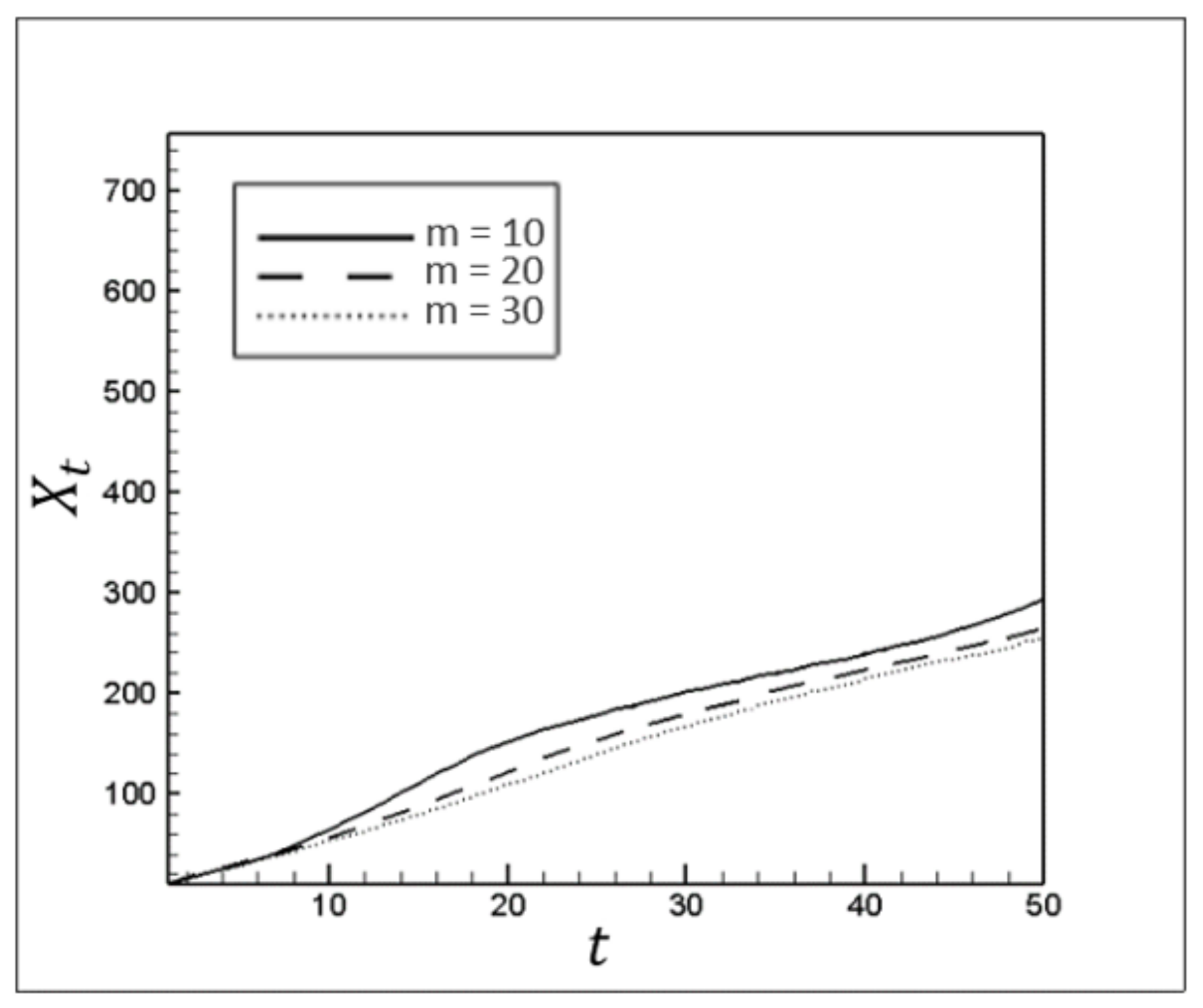
Figure 24.
The location of the advancing front at the top of the channel over time for different m.
Figure 24.
The location of the advancing front at the top of the channel over time for different m.
Figure 25.
The location of the advancing front at the bottom of the channel over time for different m.
Figure 25.
The location of the advancing front at the bottom of the channel over time for different m.
Figure 26.
The attacking front height versus time for different m.
Figure 26.
The attacking front height versus time for different m.
Figure 27.
The mean thickness of the static layer over time at the top of the channel for different m.
Figure 27.
The mean thickness of the static layer over time at the top of the channel for different m.
Figure 28.
The mean thickness of the static layer over time at the bottom of the channel for different m.
Figure 28.
The mean thickness of the static layer over time at the bottom of the channel for different m.
Figure 29.
Transverse displacement efficiency over the channel length for different m.
Figure 29.
Transverse displacement efficiency over the channel length for different m.
Figure 30.
Longitudinal displacement efficiency over the channel height for different m.
Figure 30.
Longitudinal displacement efficiency over the channel height for different m.
Table 1.
Dimensionless numbers and parameters used in simulations.
Table 1.
Dimensionless numbers and parameters used in simulations.
| m | Re | Ri | At | Ca | Inclination Angle | Pr | T |
|---|
| 20 | 100 | 1 | 0.2 | | 45 | 1 | 50 |
| Publisher’s Note: MDPI stays neutral with regard to jurisdictional claims in published maps and institutional affiliations. |
© 2021 by the authors. Licensee MDPI, Basel, Switzerland. This article is an open access article distributed under the terms and conditions of the Creative Commons Attribution (CC BY) license (https://creativecommons.org/licenses/by/4.0/).


