The Hydrodynamics and Mixing Performance in a Moving Baffle Oscillatory Baffled Reactor through Computational Fluid Dynamics (CFD)

Abstract

Oscillatory baffled reactors (OBRs) have attracted much attention from researchers and industries alike due to their proven advantages in mixing, scale-up, and cost-effectiveness over conventional stirred tank reactors (STRs). This study quantitatively investigated how different mixing indices describe the mixing performance of a moving baffle OBR using computational fluid dynamics (CFD). In addition, the hydrodynamic behavior of the reactor was studied, considering parameters such as the Q-criterion, shear strain rate, and velocity vector. A modification of the Q-criterion showed advantages over the original Q-criterion in determination of the vortices’ locations. The dynamic mesh tool was utilized to simulate the moving baffles through ANSYS/Fluent. The mixing indices studied were the velocity ratio, turbulent length scale, turbulent time scale, mixing time, and axial dispersion coefficient. We found that the oscillation amplitude had the most significant impact on these indices. In contrast, the oscillatory Reynolds number did not necessarily describe the mixing intensity of a system. Of the tested indices, the axial dispersion coefficient showed advantages over the other indices for quantifying the mixing performance of a moving baffle OBR.

Highlights:

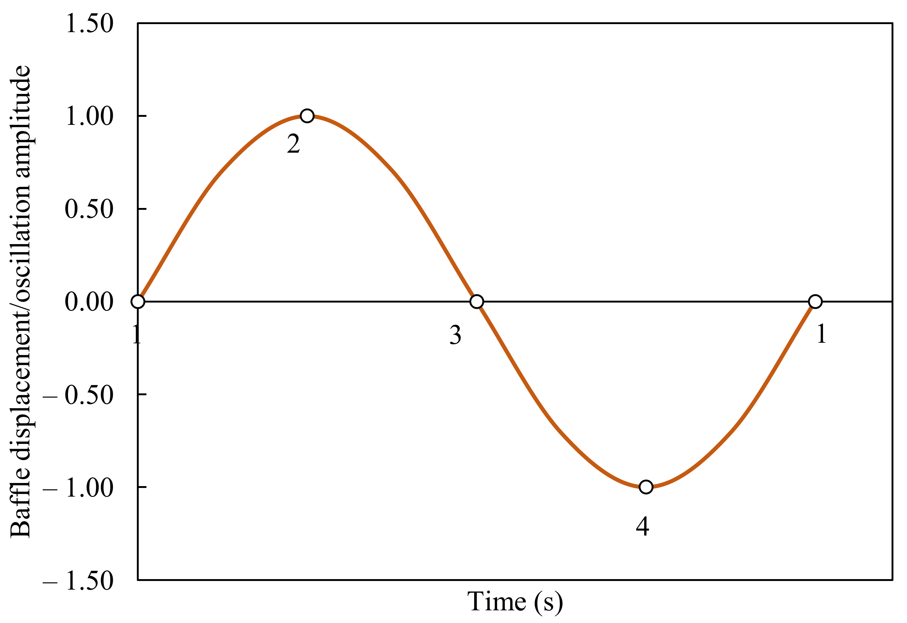
• The dynamic mesh tool is used for modeling baffle movements inside the OBR.
• Various mixing indices are compared for their ability to quantify mixing performance.
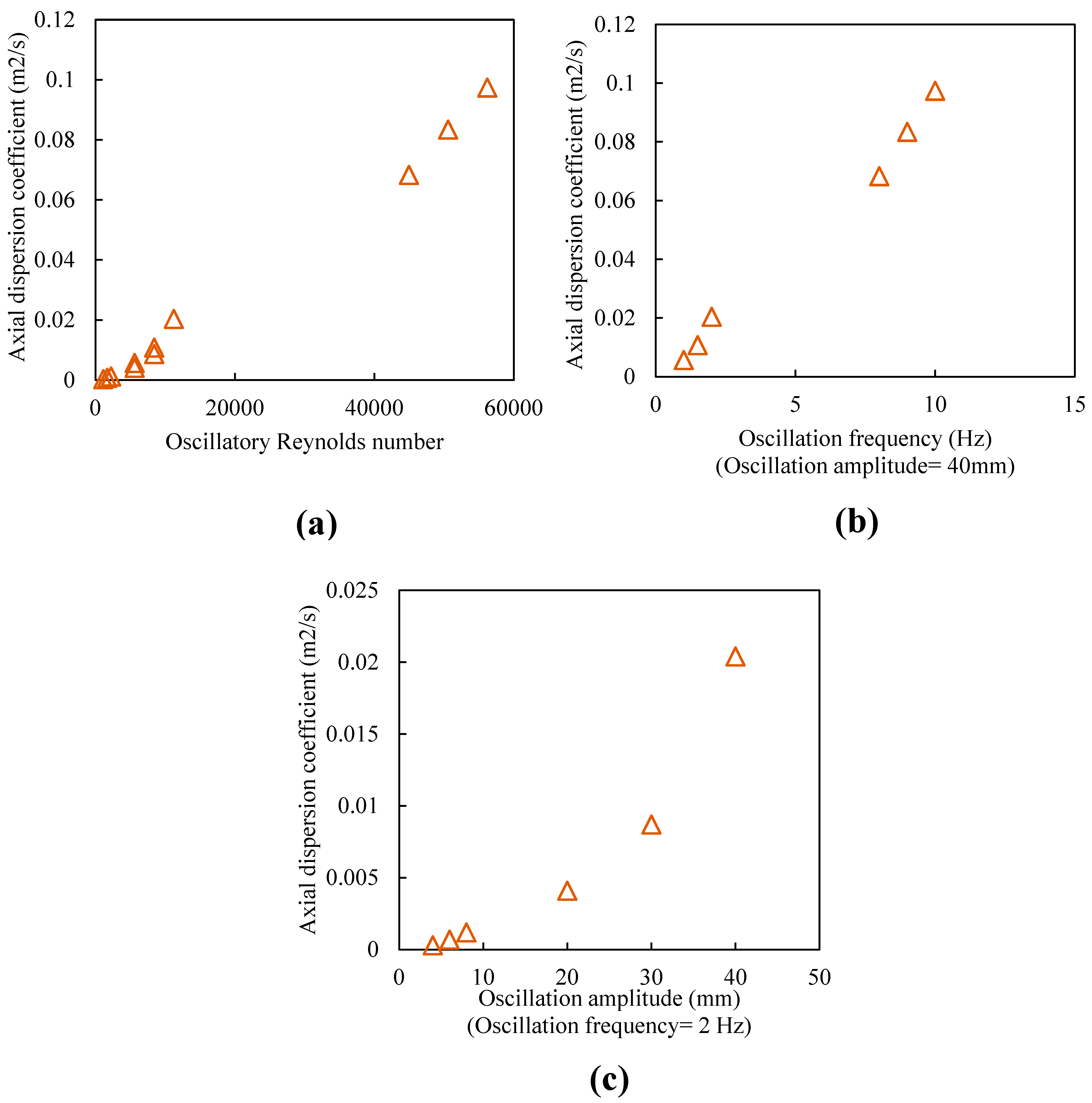
• Oscillation amplitude has a bigger impact on mixing performance than oscillation frequency.
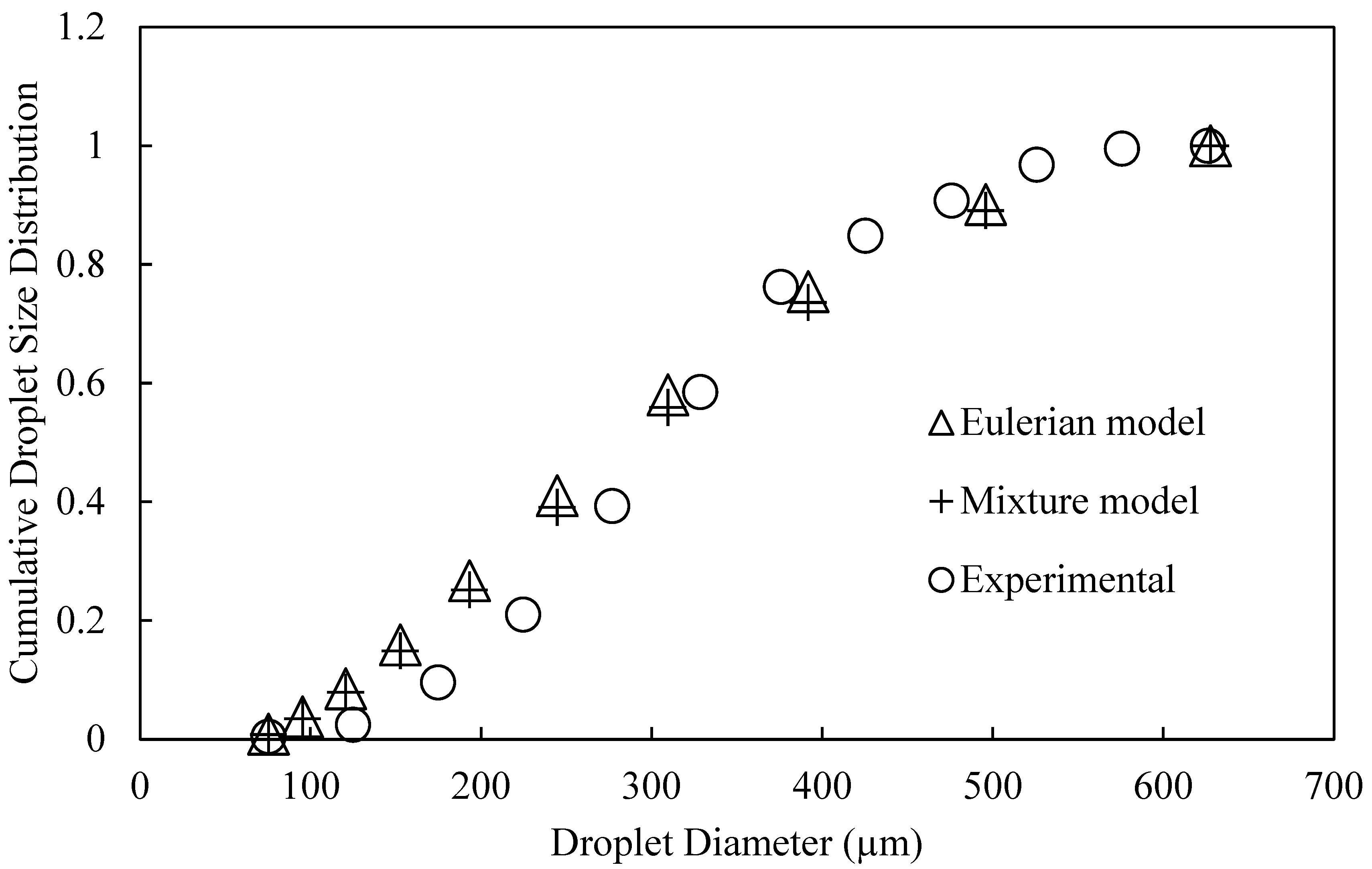
• The Eulerian model provides a better agreement to experimental data than the mixture model.
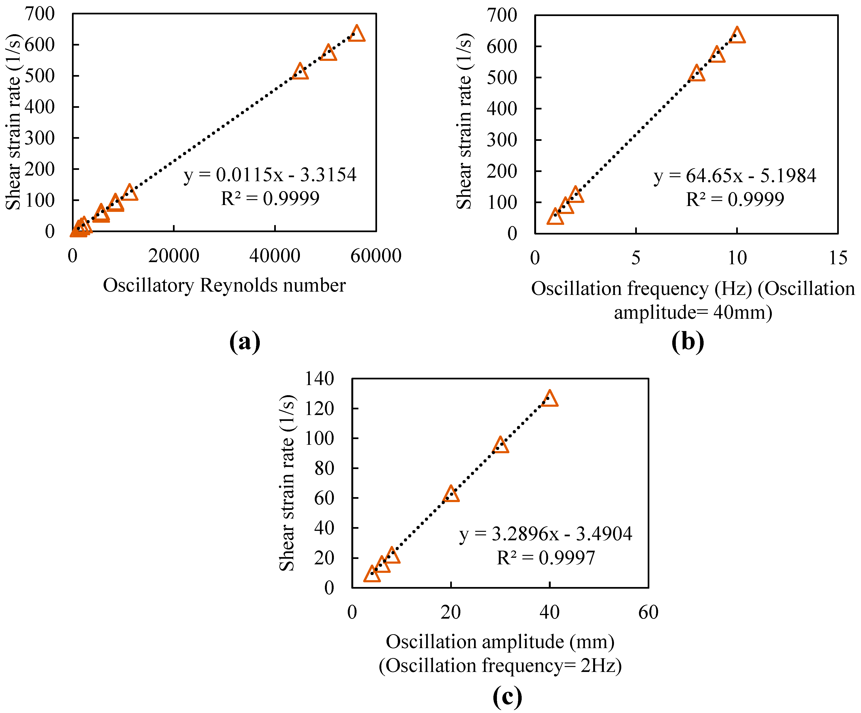
• A linear relationship between shear rate and oscillatory Reynolds number is obtained.

1. Introduction

Mixing is key to many chemical industries since it can positively affect reaction yield, mass and heat transfer, and product uniformity. Chemical industries and researchers require reactors that improve mixing, which consequently results in a more efficient production process in terms of reaction time and the quality of product [1].

The oscillatory baffled reactor (OBR) is a cylindrical column with equally spaced baffles installed transversely to a flow [2]. The reactor was first designed and introduced by Van Dijck in 1935 for liquid–liquid extraction [3]. OBR baffle designs are usually of the single orifice variety, but they may also be perforated plates and disc-and-donut [3,4]. This type of reactor can be either batch or continuous, with two methods of imparting motion to fluid: (a) through stationary baffles with moving fluid or (b) through moving baffles. In stationary baffled OBRs, fluid oscillates by means of a diaphragm, piston, or bellow, whereas in the moving baffle OBRs, baffles move via a motor and crankshaft. Typically, continuous OBRs, which are mostly of stationary baffle configuration, have been studied more due to the lower cost, waste, and energy of this type of reactor [5]. However, batch processing offers some advantages such as easier scale-up, better control of process, and better handling of toxic materials, all of which makes them still attractive for processes such as polymerization. In this study, we will study batch moving baffle OBRs.

Fluid dynamics in an OBR is mainly controlled by three dimensionless groups: i.e., oscillatory Reynolds number ($R{e}_o$), Strouhal number ($St$), and net flow Reynolds number ($R{e}_n$), which are correlated to operating parameters through Equations (1)–(3), respectively.

$$R{e}_o=2\pi f{x}_o\rho D/\mu$$

(1)

$$St=D/4\pi x_o$$

(2)

$$R{e}_n=\rho uD/\mu$$

(3)

In these groups, $D$ represents the inner diameter of the OBR, ρ is the fluid density, $u$ is the superficial fluid velocity, $\mu$ represents the fluid viscosity, $f$ is the oscillation frequency, and $x_o$ is the oscillation amplitude (center-to-peak). $R{e}_o$ is a measure of mixing intensity inside the reactor, while $St$ quantifies the effective eddy propagation and $R{e}_n$ describes the net flow intensity in continuous OBRs. The issue with this formulation for $R{e}_o$ is that it does not include all the geometrical and operational parameters involved in an OBR system. This has been addressed by Ni and Gough in 1997 by modifying the oscillatory Reynolds number as $R{e}_o^{*}=R{e}_o/\sqrt{\alpha }$ to incorporate the effect of baffle diameter, where $\alpha$ is the ratio of the area of orifice over the area of tube [6]. To include all the existing key parameters of a flow in OBR, Jimeno et al. in 2018 proposed the following correlation ($R{e}_o^{*}= \frac{u_T\rho D}{\mu }\sqrt{\frac{\beta }{\alpha }}$), where $u_T$ is the total inlet velocity including both net flow velocity and oscillatory flow velocity ($u_T=u_{net}+$ $2\pi f{x}_o$), and $\beta$ represents the ratio of optimal to user’s baffle spacing ($\beta =\frac{l_b^{opt}}{l_b}$) [7]. There is still a gap in the literature in regards to $R{e}_o$ derived specifically for a moving baffle OBR, which needs to be addressed in the future, as all the aforementioned $R{e}_o$s have been developed based on a stationary baffle OBR. However, we used Equation (1) for this study, since our geometrical parameters were fixed during the study with no net flow in the system.

In an OBR, it is possible to achieve a high level of mixing at low flow rates, since the degree of mixing in an OBR is independent of the net flow. Therefore, tubular reactors with shorter lengths can be used to reduce the size of chemical unit operations. A reduction of up to 99.6% in reactor size can be achieved as compared to continuous stirred tank reactors (STRs) with equivalent power input [2]. Moreover, OBRs are extensively scalable, as the mixing mechanisms do not change significantly from laboratory scale to industrial scale, given geometric and dynamic similarity [8]. Linear scale-up (i.e., linear correlation between mixing parameters such as axial dispersion coefficient and dimensionless numbers) is suggested for OBRs by increasing the diameter or length while maintaining $R{e}_o$, $St$, and $R{e}_n$ [9,10,11]. In addition, Anderson et al. in 2009 and Ni et al. in 2000 reported a low and uniform shear rate for OBRs compared to conventional STR [12,13]. They found up to a ten-fold reduction in shear rate when using OBRs compared to STR. Uniform mixing [5] and increased mass transfer [14,15] are the other advantages of using OBRs.

Considering the advantages of OBRs over STRs and conventional tubular reactors, considerable numbers of studies have been conducted for characterizing the mixing performance [16,17,18,19] and hydrodynamic behavior [4] of OBRs. Most studies have focused on the stationary baffle type, with very few studies done on moving baffle OBRs. Ni et al. performed some experiments in 1998 to investigate the effect of geometric parameters, such as baffle-free area (ratio of baffle orifice area to column cross-section area), baffle spacing, and baffle thickness on mixing time in a batch moving baffle OBR [20]. Using a computational fluid dynamics (CFD) approach, Manninen et al. in 2013 evaluated the mixing performance of a moving baffle OBR using the axial dispersion coefficient and velocity ratio as their parameters [21]. They reported a 10% to 17% higher axial dispersion coefficient for a moving baffle OBR than that obtained in a stationary baffle type. Gough et al. compared the flow visualization of the two types of OBR and concluded that a higher oscillation amplitude is required in the moving baffle OBR than in the stationary type in order to produce a similar flow pattern at a given oscillation frequency $\left(f\right)$ [22]. The impact of moving baffle OBRs on the rate of a catalytic hydrogenation reaction [23] and on the wax deposition processes [24] has been studied. Ni et al. in 2001 used a moving baffle OBR to perform a series of suspension polymerization processes and investigated the effect of different oscillation frequencies and amplitudes on droplet size distribution (DSD) [25]. Their study was used by Sutherland et al. to validate a CFD model of a moving baffle OBR [26]. This model was developed using an overset mesh technique for implementing baffle movements. They used their validated model to describe flow behavior in different phases of the oscillation period. Later in 2020, they were able to derive new correlations to calculate power density, oscillatory Reynolds number, and Strouhal number exclusively for a moving baffle OBR [27].

To the best of our knowledge, there is no published comprehensive study that investigates all the hydrodynamic and mixing parameters of a moving baffle OBR over a wide range of oscillation frequencies and amplitudes. Considering the lack of adequate information on moving baffle OBRs and their advantage over stationary baffle OBRs (10% to 17% higher axial dispersion coefficient for moving baffle OBRs [21]), we felt it necessary to conduct a comprehensive study on moving baffle OBRs including both the hydrodynamic and mixing aspects of this type of reactor. In addition, numerical methods have proved to be an effective tool to simulate and study various types of flow such as catalytic reactive flow [28,29], multiphase flow [26], and single phase flow [4]. Therefore, we decided to employ numerical methods—specifically, a CFD tool—to accomplish the study of the system.

The main purposes of our study are as follows: (a) to simulate a moving baffle OBR using CFD; (b) to investigate the effect of different oscillation conditions on various mixing indices, including axial dispersion coefficient, mixing time, velocity ratio, turbulent length scale, and turbulent time scale; and (c) to make a comparison among these indices in order to find the best one to represent the mixing performance of an OBR. Although turbulent length scale and turbulent time scale are mostly known as the parameters to characterize turbulence in a flow, they have been suggested as metrics for quantifying mixing quality [30,31]. In addition, hydrodynamic parameters of the system, such as velocity flow field and shear strain rate, will be investigated at different oscillation conditions.

2. CFD Model Development and Validation

In this study, a batch moving baffle OBR system (Figure 1a) was modeled and simulated using ANSYS Fluent 2019 R1. The schematic of the system (Figure 1a) shows all the details and equipment used in the process. For simplification, only the column and baffles were considered for creating the geometry, which is shown in Figure 1b. The column had a diameter and height of 50 and 654 mm, respectively, and there were 8 orifice baffles that moved fluid sinusoidally. The orifice diameter was 24 mm, the space between baffles was 75 mm, and the baffle clearance was 2 mm. The effect of rods was neglected, since Ni et al. described them as smooth rods with no appendages [25]. Sutherland et al. also neglected the effect of baffle clearance (the gap between the baffles and the reactor wall) on the performance of a moving baffle OBR in their study [26]. However, in our study, the baffle clearance was modeled, since baffle clearance can affect the hydrodynamics of the column and thus the particle size distribution [15].

The materials used in our model for a liquid–liquid suspension system included a continuous, organic phase (density = 760 kg/m³; viscosity = $1.7\times {10}^{-3} \mathrm{Pa}.\mathrm{s}$) consisting of Isopar oil and stabilizer, plus a dispersed, aqueous phase (density of 1038 kg/m³; viscosity = $2.8\times {10}^{-3} \mathrm{Pa}.\mathrm{s}$) of water and acrylamide. The volume fraction of aqueous phase was 19.86%; refer to Ref. [25] for more information about the system.

A two-dimensional (2D) axisymmetric geometry was created for the entire reactor. Although there are studies [32,33] indicating that axisymmetric models cannot fully describe these reactors, Reis et al. in 2005 reported very good agreement between an axisymmetric 2D model and experimental data, in terms of mixing performance [34]. Furthermore, Sutherland et al. [26] showed that the axisymmetric assumption is acceptable for such a system by validating their model with experimental droplet size distribution data obtained from Ref. [25].

Figure 1c shows a close-up view of the mesh generated by ANSYS 2019 meshing. The triangle method and inflation layer were applied at wall and baffle boundaries, which result in high mesh quality (160,607 elements with the grid size of 0.5 mm). A finer mesh (smaller-sized elements) was created near the walls to accommodate the intense flow changes in those regions. The variable time step method was chosen in the range of 10⁻⁴ and 10⁻⁵ to satisfy $Co=\frac{u\Delta t}{\Delta x} \le 1$ [35], as this criterion is necessary for convergence in solving certain partial differential equations numerically.

To model the periodic movement of the baffles along the reactor, we used the dynamic mesh method. This mesh technique can model geometries that change with flow time. This technique updates the mesh automatically as the boundary condition moves [36]. Different methods can be adopted for dynamic mesh in ANSYS Fluent including Smoothing, Layering, and Remeshing [37]. Smoothing and Remeshing methods were applied to simulate baffled motion considering that the mesh is created using the triangle method. The dynamic mesh technique has shown good reliability in modeling systems with moving parts [37,38,39]. Therefore, this technique can be relied upon for modeling moving parts in CFD.

Considering the sinusoidal motion of baffles, a user-defined function (UDF) was created based on Equation (4):

$$u_{baffle}=2\pi f\left(x_0\right)\cos \left(2\pi ft\right)$$

(4)

where $u_{baffle}$, $f$, and $x_0$ are the baffle velocity, oscillation frequency, and oscillation amplitude, respectively.

The next step in modeling flow was to determine its intensity and apply suitable models for simulation based on flow conditions. Therefore, $R{e}_o$ was used for determining the flow condition and the intensity of mixing in the reactor. According to Harvey et al., for $R{e}_o$ over 5000, intense mixing (i.e., turbulent flow) is achieved and for 50 < $R{e}_o$ < 500, soft mixing occurs (i.e., no radial mixing occurs inside reactor) [40]. The oscillation conditions (

Table 1. Operating conditions used in the study.

Oscillation Frequency (Hz)	Oscillation Amplitude (mm)	$\mathit{R}{\mathit{e}}_{\mathit{o}}$	$\mathit{S}\mathit{t}$
10	40	56,179	0.0995
9	40	50,561	0.0995
8	40	44,943	0.0995
2	40	11,235	0.0995
1.5	40	8426	0.0995
1	40	5618	0.0995
2	30	8427	0.1326
2	20	5618	0.1989
2	8	2247	0.4974
2	6	1685	0.6631
2	4	1124	0.9947

) used in our study suggested that none of oscillation conditions provided $R{e}_o$ in the range of soft mixing. Hence, turbulent conditions were considered for all the oscillation conditions applied. Generally, there are two families of methods for modeling turbulence in ANSYS Fluent: Reynolds-averaged Navier–Stokes (RANS) methods and Scale Resolving Simulation (SRS) methods. It is stated that RANS models are more suitable for steady-state flow, and SRS suits transient flow better. However, there are studies that have been able to successfully model different transient turbulent flows using the RANS method such as CFD modeling of a gas-liquid STR using $k-\epsilon$, which is of RANS methods [41], and modeling of a liquid-liquid moving baffle OBR using $k-\epsilon$ [26]. Ekambara and Dhotre in 2007 also reported very good agreement between experimental and numerical data when they employed a $k-\epsilon$ turbulence model to simulate a gas-liquid flow inside a stationary baffle OBR [42]. In addition, RANS turbulence models are the only options when the population balance model is applied in ANSYS Fluent.

For a 2D unsteady, turbulent system and Newtonian fluid, the flow is governed by Reynolds-averaged Navier-Stokes (RANS) equations. Therefore, the continuity equation is:

$$\frac{\partial \overline{u_i}}{\partial x_i}=0$$

(5)

and the momentum conservation equations for the x-direction and y-direction are:

$$\frac{\partial \overline{u_i}}{\partial t}+\overline{u_j}\frac{\partial \overline{u_i}}{\partial x_j}=-\frac{\partial \overline{P}}{\partial x_i}+\nu \frac{{\partial }^2\overline{u_i}}{\partial x_j\partial x_j}-\frac{\partial \left(\overline{u_i’u_j’}\right)}{\partial x_j}$$

(6)

where $\overline{P}$ is mean pressure and $\overline{u_i}$ and $\overline{u_i’}$ represent the average and fluctuating components of velocity, respectively. $\overline{u_i’u_j’}$ is the stress term that incorporates the turbulence characteristics of the flow.

To describe the turbulence of the flow in our system, a (Renormalization Group) RNG $k-\epsilon$ turbulent model was utilized, which is a modification on a standard $k-\epsilon$ model. The standard $k-\epsilon$ model uses two main parameters to formulate turbulent flows: turbulent kinetic energy ($k$) and turbulent energy dissipation ($\epsilon$). These two parameters will be discussed later and used to calculate turbulent length scale and turbulent time scale, which are of great importance in studying the mixing performance of a system. The RNG $k-\epsilon$ model was created using Renormalization Group (RNG) methods by Yakhot et al. to renormalize Navier-Stokes equations in order to include the effects of smaller scales of motion [43]. Equations (7) and (8) were used to model the turbulence using RNG $k-\epsilon$ [43]:

$$\frac{\partial }{\partial t}\left(\rho k\right)+\frac{\partial }{\partial x_i}\left(\rho k{u}_i\right)=\frac{\partial }{\partial x_j}\left[\rho \left(\nu +\frac{{\nu }_T}{{\sigma }_k}\right)\frac{\partial k}{\partial x_j}\right]+G_k-\rho \epsilon$$

(7)

and

$$\frac{\partial }{\partial t}\left(\rho \epsilon \right)+\frac{\partial }{\partial x_i}\left(\rho \epsilon u_i\right)=\frac{\partial }{\partial x_j}\left[\rho \left(\nu +\frac{{\nu }_T}{{\sigma }_{\epsilon }}\right)\frac{\partial \epsilon }{\partial x_j}\right]+C_{1\epsilon }\frac{\epsilon }{k}{G}_k-C_{2\epsilon }\rho \frac{{\epsilon }^2}{k}$$

(8)

In these equations, ${\nu }_T=C_{\mu }{k}^2/\epsilon$ is the kinematic eddy viscosity, $G_k$ is the generation of turbulence kinetic energy due to the mean velocity gradients, and $C_{1\epsilon }=1.44$, $C_{2\epsilon }=1.92$, $C_{\mu }=0.09$, ${\sigma }_k=1.0$, and ${\sigma }_{\epsilon }=1.3$ are constants [43].

Reynolds-averaged Navier-Stokes (RANS) and RNG $k-\epsilon$ equations are only applicable in single-phase systems and for them to be utilized for a multiphase medium, a Euler-Euler approach was applied. In the Euler-Euler approach, different phases are treated mathematically as interpenetrating continua, and the occupancy of each phase is accounted in terms of respective fraction of total fluid [26].

There are three different Euler-Euler multiphase models in ANSYS Fluent: the volume of fluid (VOF) model, the mixture model, and the Eulerian model. Among the Euler-Euler multiphase models, the Eulerian model was selected to describe the multiphase flow in our study, which showed slightly more accurate agreement with experimental data than the mixture model for this specific study, as will be demonstrated later in this section.

The flow in this study was considered to be a dispersed liquid-liquid phase, in which the dispersed phase includes a wide range of droplet sizes. These droplets with different diameters can interact with each other through the aggregation and breakage mechanisms.

To take droplet size distribution into account, a population balance model was used since it can account for aggregation and breakage in dispersed multiphase flows [42]. A general form of the population balance equation is [44]:

$$\frac{\partial n_i}{\partial t}+\nabla .\left(u_{DP}{n}_i\right)=B_B+B_A-D_B-D_A$$

(9)

where $u_{DP}$ is the dispersed phase velocity, $n_i$ is the number density of size group $i$, $B_B$ and $D_B$ represent the birth and the death rate due to breakage, and $B_A$ and $D_A$ are the birth and the death rate due to aggregation. Since the OBR in this study is a batch reactor, there is no inlet and outlet flow, and therefore, no source term has been included. In addition, there is not any growth phenomenon other than aggregation to be considered due to the non-reacting nature of the process. The droplet number density $n_i$ is related to the dispersed phase volume fraction ${\epsilon }_G$ by [44]:

$${\epsilon }_G{f}_i=n_i{V}_i$$

(10)

where $f_i$ and $V_i$ represent the volume fraction and the corresponding volume of droplets of group $i$, respectively.

The Luo model [45] was applied for both breakage and aggregation phenomena. For the breakage, a binary breakage of the droplet is assumed and a dimensionless parameter for describing the size of the daughter droplet (the breakage volume fraction) has been introduced as follows [45]:

$$f_{BV}=\frac{V_i}{Vol}=\frac{d_i^3}{d^3}=\frac{d_i^3}{d_i^3+d_j^3}$$

(11)

In the equation above, $d_i$ and $d_j$ represent diameters (corresponding to $V_i$ and $V_j$) of the daughter droplet in the binary breakage of a parent bubble with diameter $d$ (corresponding to volume $Vol$). The breakage rate of the droplets of volume $V_j$ into volume sizes of $V_i \left(=Vol\times f_{BV}\right)$ is calculated by [45]:

$$\frac{{\mathsf{\Omega }}_B\left(V_j:V_i\right)}{\left(1-{\epsilon }_G\right)n_j}=C{\left(\frac{\epsilon }{d_j^2}\right)}^{1/3}{{\displaystyle \int }}_{{\xi }_{min}}^1\frac{{\left(1+\xi \right)}^2}{{\xi }^{11/3}}\times \exp \left(-\frac{12c_f\sigma }{\beta {\rho }_L{\epsilon }^{\frac{2}{3}}{d}_j^{\frac{5}{3}}{\xi }^{\frac{11}{3}}}\right)d\xi$$

(12)

where $\xi =\lambda /d_j$ is the size ratio between an eddy and a particle in the inertial sub-range and therefore ${\xi }_{min}={\lambda }_{min}/d_j$. $C$ and $\beta$ are 0.923 and 2.0, respectively, which were obtained from the consideration of droplets breakage in turbulent dispersion systems in Ref [45], and $c_f$ is the increased coefficient of the surface area, which can be obtained as [45]:

$$c_f=\left[f_{BV}^{\frac{2}{3}}+{\left(1-f_{BV}\right)}^{\frac{2}{3}}-1\right]$$

(13)

The birth rate of group $i$ bubbles due to the breakage of larger bubbles is obtained by:

$$B_B={{\displaystyle \sum }}_{j=i+1}^N{\mathsf{\Omega }}_B\left(V_j:V_i\right)n_j$$

(14)

The death rate of group $i$ bubbles due to breakage is obtained by:

$$D_B={\mathsf{\Omega }}_{Bi}{n}_i$$

(15)

where

$${\mathsf{\Omega }}_{Bi}={{\displaystyle \sum }}_{i=1}^N{\mathsf{\Omega }}_{Bki}$$

(16)

In the Luo model, the aggregation rate is defined as the rate of particle volume formation due to binary collisions of particles with volumes $V_i$ and $V_j$ [36]:

$${\mathsf{\Omega }}_A\left(V_i,,,V_j\right)={\omega }_A\left(V_i,,,V_j\right)P_A\left(V_i,,,V_j\right)$$

(17)

where $P_A\left(V_i,V_j\right)$ is the probability aggregation due to collision and ${\omega }_A\left(V_i,V_j\right)$ is the frequency of collision, which is given by:

$${\omega }_A\left(V_i,V_j\right)=\frac{\pi }{4}{\left(d_i+d_j\right)}^2{\overline{u}}_{ij}$$

(18)

where ${\overline{u}}_{ij}$ is the characteristic velocity of collision of two particles with diameters $d_i$ and $d_j$, which is obtained by:

$${\overline{u}}_{ij}={\left({\overline{u}}_i^2+{\overline{u}}_j^2\right)}^{1/2}$$

(19)

where

$${\overline{u}}_i=1.43{\left(\epsilon d_i\right)}^{1/3}$$

(20)

The expression for the probability of aggregation is defined as:

$$P_A=\exp \left\{-c_1\frac{{\left[0.75\left(1+x_{ij}^2\right)\left(1+x_{ij}^3\right)\right]}^{1/2}}{{\left(\frac{{\rho }_2}{{\rho }_1}+0.5\right)}^{\frac{1}{2}}{\left(1+x_{ij}\right)}^3}W{e}_{ij}^{1/2}\right\}$$

(21)

where $c_1$ represents a constant of order unity, ${\rho }_1$ and ${\rho }_2$ are the densities of the primary and secondary phases, respectively,$x_{ij}=d_i/d_j$, and the Weber number is determined as follows:

$$W{e}_{ij}=\frac{{\rho }_i{d}_i{\left({\overline{u}}_{ij}\right)}^2}{\sigma }$$

(22)

The solution for the aforementioned governing equations for the mass and momentum conservation of each phase, along with the population balance equations, was sought. A phase-coupled SIMPLE (Semi-Implicit Method for Pressure Linked Equations) algorithm was applied to couple pressure and velocity, and a first-order discretization method was chosen for the time discretization. To discretize the population balance equation, a finite series of size ranges was implemented to follow the form of Lister et al.’s geometric ratio [46]. This method divides the size range of droplet into a series of ‘bins’ through the correlation indicated in the following:

$$\frac{v_{i+1}}{v_i}=2^q$$

(23)

where q is the geometric ratio and $v$ represents the volume of each droplet bin size. In the current study, droplets ranging from 75 to 628 µm diameter are divided into 10 bins, as illustrated in

Table 2. Droplet size for each bin used in the study.

Bin Number	1	2	3	4	5	6	7	8	9	10
Droplet size (µm)	75	95	121	152	193	244	309	392	496	628

. For this discretization, q is 1.02.

The model was run for an adequate time so that the periodical behavior was established throughout the reactor. At that point, all the parameters in every single point of the reactor should show a periodic behavior. The flow is considered as periodic when the values for a specific parameter such as velocity or pressure at selected monitoring points converged upon a repeating trend during an oscillation cycle. Figure 2 shows the velocity magnitude at the center point of the reactor against oscillation time for 2 Hz of oscillation frequency and 40 mm of oscillation amplitude, and it shows that it takes almost four oscillation cycles before the reactor shows a periodic behavior.

To ensure our model could realistically mimic the actual reactor, droplet size distributions (DSDs) were obtained by averaging DSD data over an oscillation period considering 2 Hz of oscillation frequency and 40 mm of oscillation amplitude for baffles movement. Size distribution has been used as a parameter for validating numerical models in the literature: when methyl methacrylate particle size distribution was used to validate a CFD model of a stirred tank reactor [47]; when bubble size distribution was used to validate a numerical model for a bubble column [48]; and when DSD was used to validate a numerical model of an OBR [26]. Therefore, DSD data were compared with the experimental DSD data presented by Ni et al. [25] using two different multiphase models i.e., the Mixture and Eulerian, which is illustrated in Figure 3. In this figure, the cumulative DSD was chosen over regular DSD for presenting the data, since a population balance model can only provide certain values for bin sizes over a bin size range, which does not necessarily match experimental bin sizes. Therefore, according to Figure 3, it can be observed that the Eulerian model showed slightly more reasonable agreement with experimental data than the Mixture model.

In order to make sure that our results were independent of grid size, three different grids with 81,450, 160,607, and 317,904 cells were employed using the axial velocity profiles at the center cross-section (axially) of the reactor in the oscillation condition of 40 mm of amplitude and 2 Hz of frequency. We chose 5 s after the start of simulation (equal to 10 oscillation cycles) to capture the profiles. Figure 4 shows the comparison along with the number of cells for each case. In this plot, we considered 26 equally spaced points along the center cross-section of the reactor to be able to perform a normalized root mean square error (NRMSE) comparison among the profiles. NRMSE is defined as $NRMSE= \frac{\sqrt{({{\displaystyle \sum }}_{i=1}^n{\left(H\left(i\right)-J\left(i\right)\right)}^2)/n}}{J_{max}-J_{min}}$, where $H\left(i\right)$ and $J\left(i\right)$ are two different sets of data, n is the number of data points, and $J_{max}$ and $J_{min}$ are the maximum and minimum values, respectively. All three profiles match perfectly in the region of radius = 0.005–0.025 m. For radii between 0 and 0.005 m, a discrepancy is observed when comparing the axial velocities of a rough grid (81,450 cell grid) with the other two profiles. The reason of the discrepancy at the center region of the column is the high velocity of flow in those locations (radius = 0–0.005 m), which need a higher-resolution grid to capture the correct velocity. However, the axial velocity profiles related to the fine grid (317,904 cell grid) and moderate grid (160,607 cell grid) match perfectly with NRMSE = 0.0084, while the NRMSE value produced by comparing rough and moderate mesh profiles is 0.0527. Therefore, it can be concluded that our model is independent of grid size for mesh grids with 160,607 or more cells.

Our validation experiments (as described in this section) allowed us to establish a set of oscillation frequencies and oscillation amplitudes (Table 1) for the next series of studies. The choice of operating conditions was based on their feasibility in experimental works accomplished thus far in the literature [20,25]. In addition, the second phase (aqueous phase) was eliminated from the fluid, and we used pure Isopar as a working fluid, henceforth. All the other conditions, including geometry, meshing, and boundary conditions, remained unchanged. CFD models were run for all the operating conditions for an adequate time so that periodic behavior was established throughout the reactor. Once values for velocity and pressure at selected monitoring points converged upon a repeating trend during an oscillation cycle, we knew that the periodic flow pattern was fully established and the effect of start-up on the system flow was completely removed.

3. Results and Discussion

Our goal was to perform a comprehensive study of the mixing performance and hydrodynamic behavior of a moving baffle OBR. To do that, several mixing indices and hydrodynamic parameters were employed, and the mixing performance was justified using hydrodynamic data obtained from CFD simulations. In addition, a comparison was made on mixing indices to determine the best one that is not only able to represent the mixing performance of the reactor but can be easily calculated as well.

Mixing indices can be categorized into two groups based on their calculation method. The first group includes the velocity ratio, turbulent length scale, and turbulent time scale, which do not need a tracer added to the reactor in order to be calculated, and the second group has a mixing time and axial dispersion coefficient that require a tracer for calculating their values.

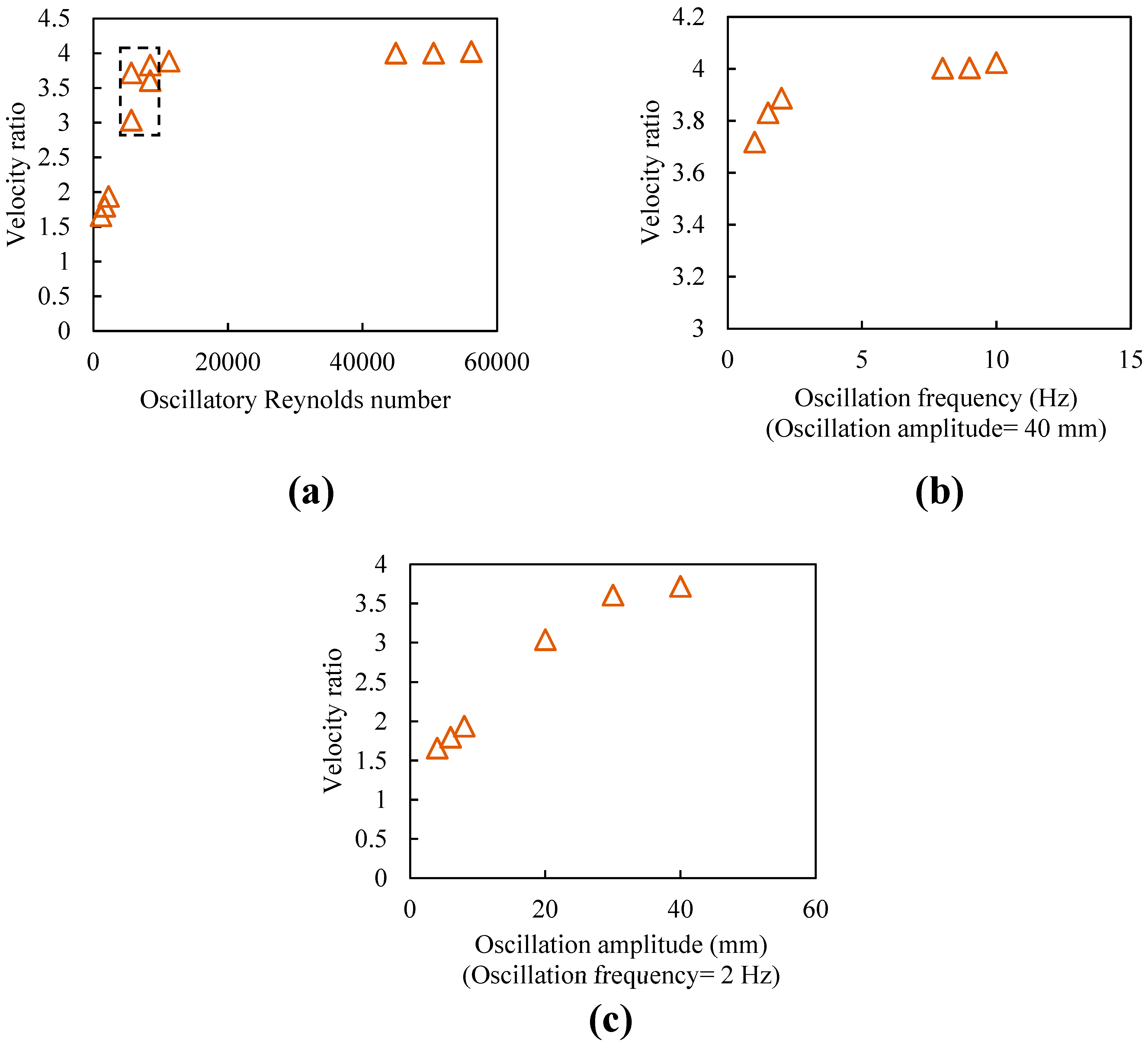
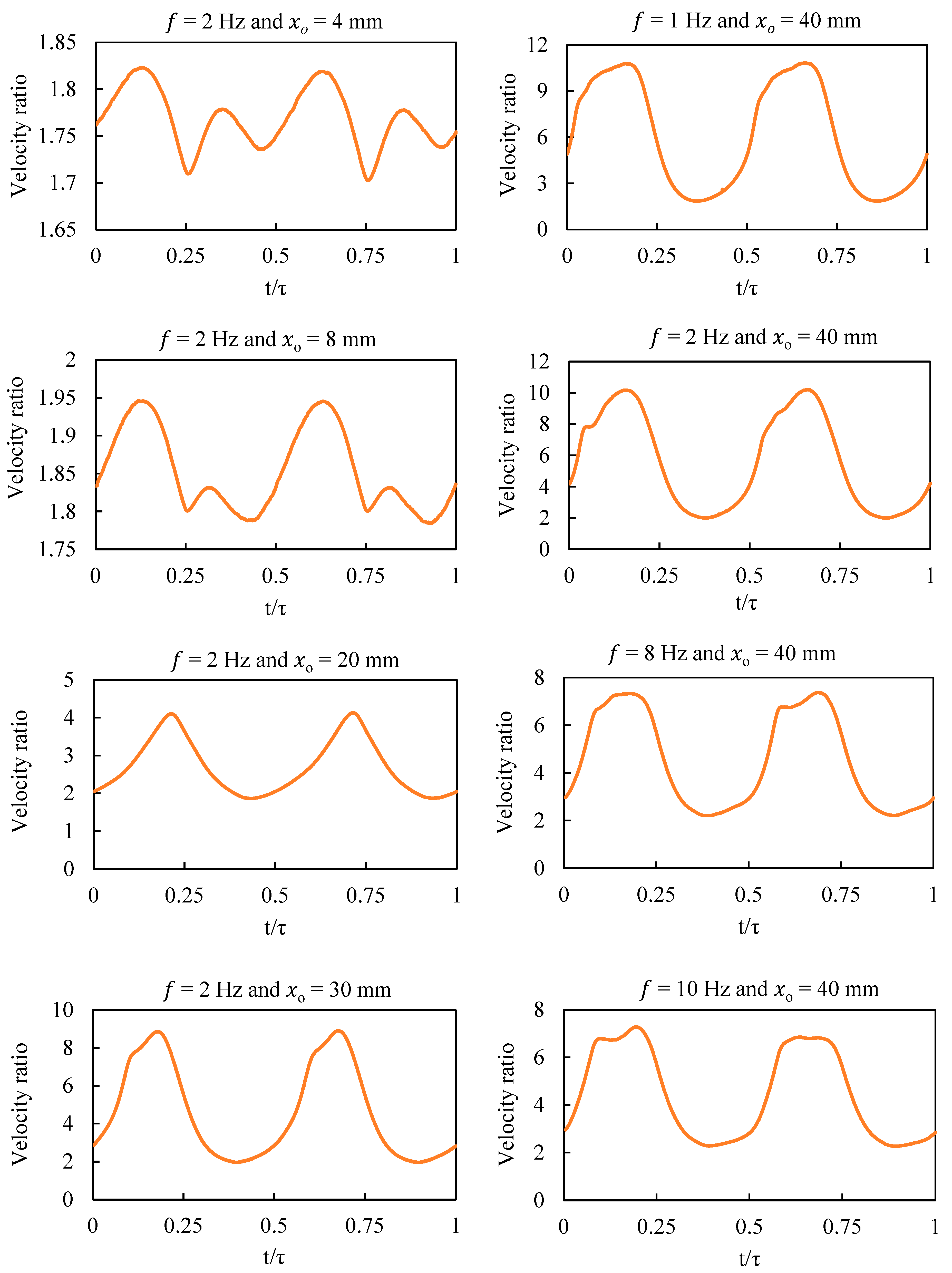
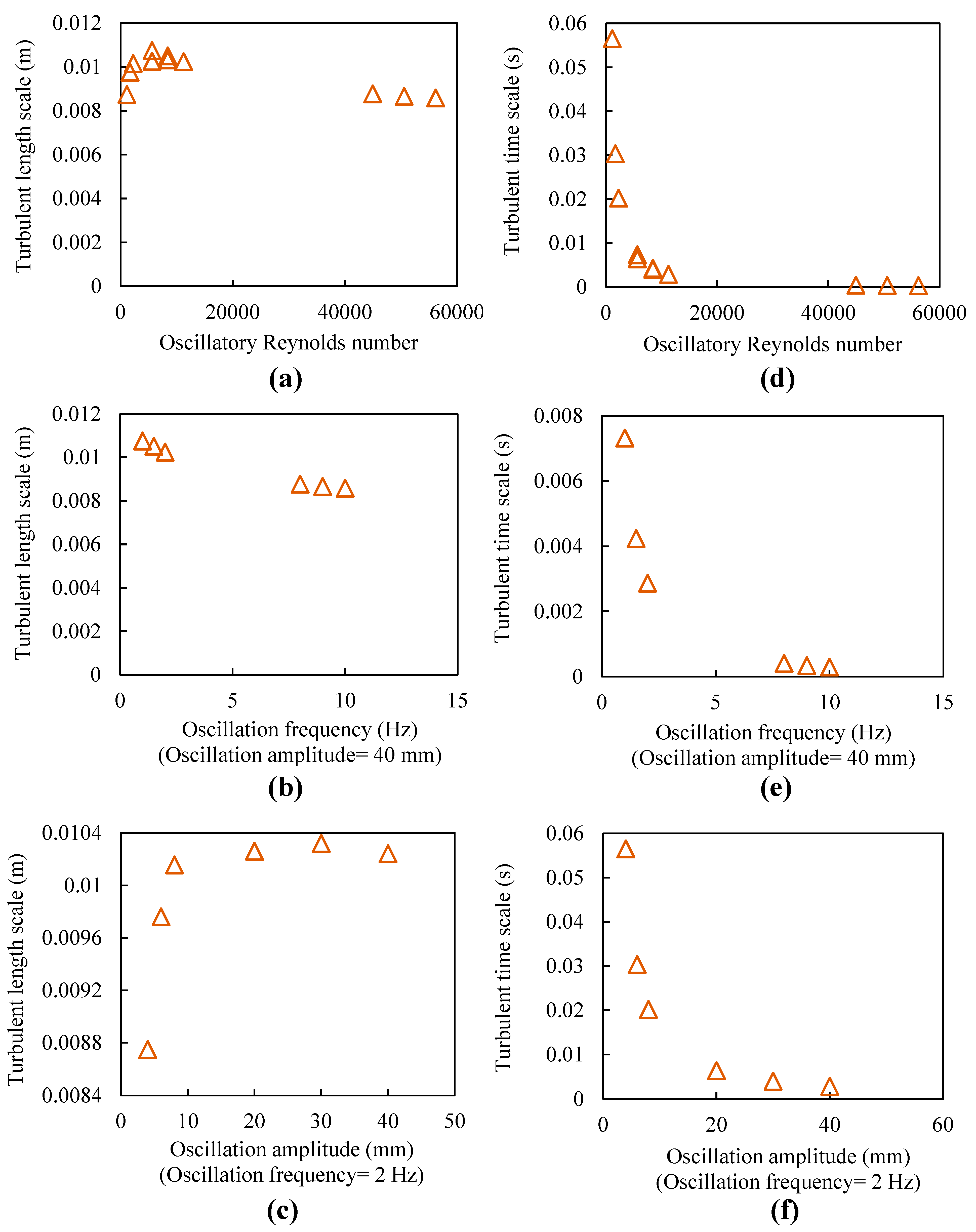
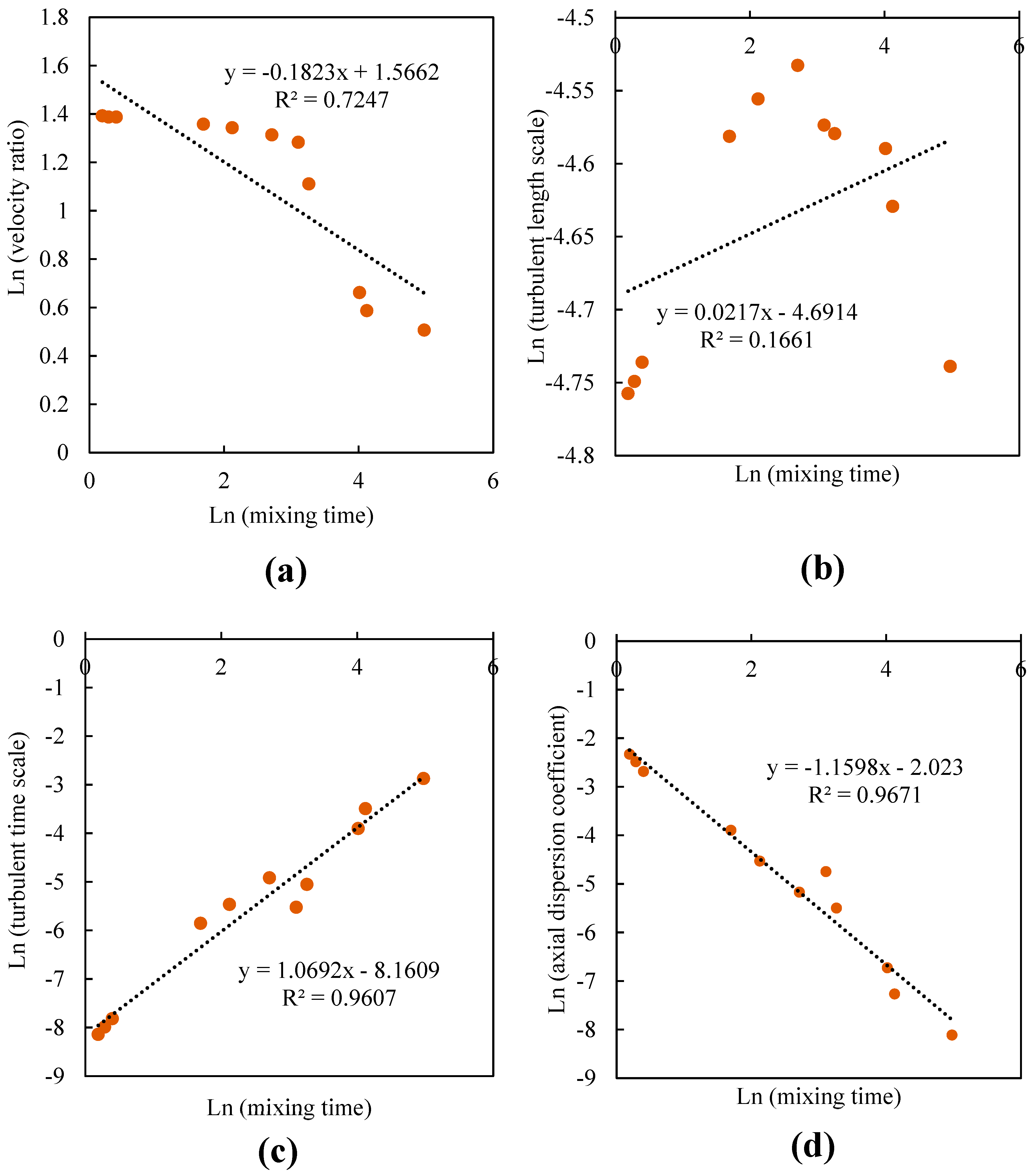
3.1. Velocity Ratio, Turbulent Length Scale, and Turbulent Time Scale

The velocity ratio is a mixing parameter in OBR that has been used to compare the mixing performance of Newtonian and non-Newtonian fluids [16,21], investigate the effect of OBR geometry on mixing [31], or as a parameter for scale-up purposes [10]. The equation for calculating the velocity ratio is:

$$R_V\left(t\right)=\frac{{{\displaystyle \sum }}_i\left|u_{i,axial}\right|V_{cell,i}}{{{\displaystyle \sum }}_i\left|u_{i,radial}\right|V_{cell,i}}$$

(24)

where $V_{cell,i}$ is the volume of the computational cell (m³) and $R_V\left(t\right)$ represents the velocity ratio, which is time dependent; therefore the numerical values reported need to be averaged over time. It should be noted that the instantaneous value of $R_V$ can be rather high. Therefore, Manninen et al. [21] suggested the time average of $1/R_V$ instead of $R_V$ in order to lower the effect of high $R_V$ values as follows:

$$R_V={\left(\frac{1}{\Delta t}\underset{t_0}{\overset{t_0+\Delta t}{{\displaystyle \int }}}\frac{dt}{R_V\left(t\right)}\right)}^{-1}$$

(25)

The index describes the effective transport of the axial oscillatory velocity component to the radial velocity, where the lower the value, the more effective the mixing [21].

Figure 5 shows the trend of velocity ratio against oscillatory Reynolds number, oscillation frequency, and oscillation amplitude. This figure shows that as $R{e}_o$ increased, the velocity ratio approached 4. The velocity ratio ranged between 1.6 and 4 for 1123 < $R{e}_o$ < 56,179. Fitch et al. in 2005 reported the velocity ratio range between 2 and 3.8 for a stationary baffle OBR and suggested that the velocity ratio approaches 2 [16]. It should be noted that all geometry parameters of the work done by Fitch et al. [16] were the same as those of our work except for reactor height, whose change does not have a huge impact on the mixing performance and hydrodynamic behavior of the reactor because of the similarity of the velocity pattern in each inter-baffle area. The difference between the velocity ratio value in our study and those in the work done by Fitch et al. [16] was expected because the application of motion varied from moving baffle OBR to stationary baffle type.

Figure 5a shows that the velocity ratio was not a strong function of oscillatory Reynolds number in high oscillatory Reynolds numbers ($R{e}_o$ > 8000). In addition, this figure shows that OBRs with the same $R{e}_o$ numbers did not necessarily have similar behavior in terms of mixing performance (refer to the rectangle inside Figure 5a). The velocity ratio was independent of oscillation frequency at high frequencies (Figure 5b). Figure 5c shows that oscillation amplitude had a stronger impact on velocity ratio than frequency, and an almost linear relationship can be seen between velocity ratio and amplitude for amplitudes less than 30 mm.

Figure 6 illustrates the trend of velocity ratio over time during one oscillation period. While most oscillation frequencies and amplitudes showed two peaks during the oscillation period, the cases with low oscillation amplitudes showed four peaks; this could be the effect of gravity, which has a significant impact on low velocity flow. The cases with the same oscillation amplitude and different oscillation frequencies illustrated an almost similar trend for velocity ratio, whereas the cases with the same oscillation frequency and different oscillation amplitudes did not exhibit similarity in the trend of velocity ratio. In addition, the increase of oscillation amplitude caused the velocity ratio peak values to increase, while the velocity ratio peak values did not increase for oscillation frequencies greater than 8 Hz. This can explain why the oscillation frequency does not have a significant impact on the velocity ratio, which will be discussed in the next section.

In turbulent flow, the largest eddies carry most of the momentum and energy, while the smallest eddies (Kolmogorov scale) dissipate energy into heat [7]. The Taylor microscale falls in between the large-scale eddies and the small-scale eddies [7].

The turbulent length scale is the distance over which fluid elements are moved due to the turbulent eddies of this kinetic energy. Ni et al. claimed that the turbulent length scale can be considered as a measure for the mixing rate and concluded that the higher the mixing length, the more intense the turbulent mixing. The turbulent length scale is comparable to the characteristic length scale of any system, which is given by [30]:

$$l=\frac{k^{3/2}}{\epsilon }$$

(26)

where $k$ is turbulent kinetic energy and ε represents the turbulent dissipation rate, as discussed in the previous section.

Another index used in the literature for quantifying the mixing performance of a reactor is the turbulent time scale, which can be calculated as follows [31]:

$$t_k={\left(\frac{\mu }{\rho \epsilon }\right)}^{1/2}$$

(27)

where $\mu$ is viscosity and $\rho$ is density. $t_k$ is the smallest time scale of turbulence, and its importance is more highlighted in controlling chemical reactions whose reaction time is not greater than those of turbulent time scales [31]. Ni et al. also believed that turbulent length and time scales affect the droplet formation and subsequently size distribution in the OBR [31]. Turbulent length scale and turbulent time scale have been used as mixing indices by Ni et al. in 2003 [30] and in 2004 [31].

The turbulent length scale and turbulent time scale values in our operating conditions are illustrated in Figure 7. It can be seen that the turbulent length scale in the OBR ranged between 0.008 and 10⁻² m, and the turbulent time scale ranged from 0.3 to 56 ms; both ranges mentioned are aligned with the values reported by Jimeno et al. [7] and Ni et al. [31] for stationary baffle OBRs, which shows that both the moving baffle and stationary baffle OBRs exhibit similar ranges of values for turbulent length scale and turbulent time scale. The values of our turbulent length scale also agree with the concept of mixing length, which should be less than the baffle spacing (the characteristic length of the system), as discussed by Jimeno et al. [7].

Furthermore, we found no meaningful relationship between turbulent length scale and oscillatory Reynolds number. This is the phenomenon that Ni et al. also discussed in their study of a stationary baffle OBR, and they could not explain the reason behind that [25]. However, the turbulent length scale increased with the increase of oscillation amplitude, especially with low amplitudes and constant frequency. In addition, it decreased so slightly with the increase of oscillation frequency that the impact of oscillation frequency on turbulent length scale can be neglected.

Unlike the turbulent length scale, the turbulent time scale showed similar trends in relation to changes in oscillatory Reynolds number, oscillation amplitude, and oscillation frequency, as shown in Figure 7. However, this parameter was also more dependent on oscillation amplitude. McDonough et al. reported the micromixing time (which is somehow equivalent to turbulent time scale) for a meso-scale stationary baffle OBRs. Despite the different values of the parameters in their work comparing to the turbulent time scale in this study, the micromixing time with oscillatory Reynolds number trend is very similar to the trends shown in Figure 7 [49]. They both show large values for the turbulent time scale in low oscillatory Reynolds numbers and approach zero values in high oscillatory Reynolds numbers. This adds more validity to our work, as it almost repeats an experimental trend. It should be mentioned that the actual values of these two parameters are not comparable due to the differences between the reactors and also the difference between the methods of calculation (numerical and experimental).

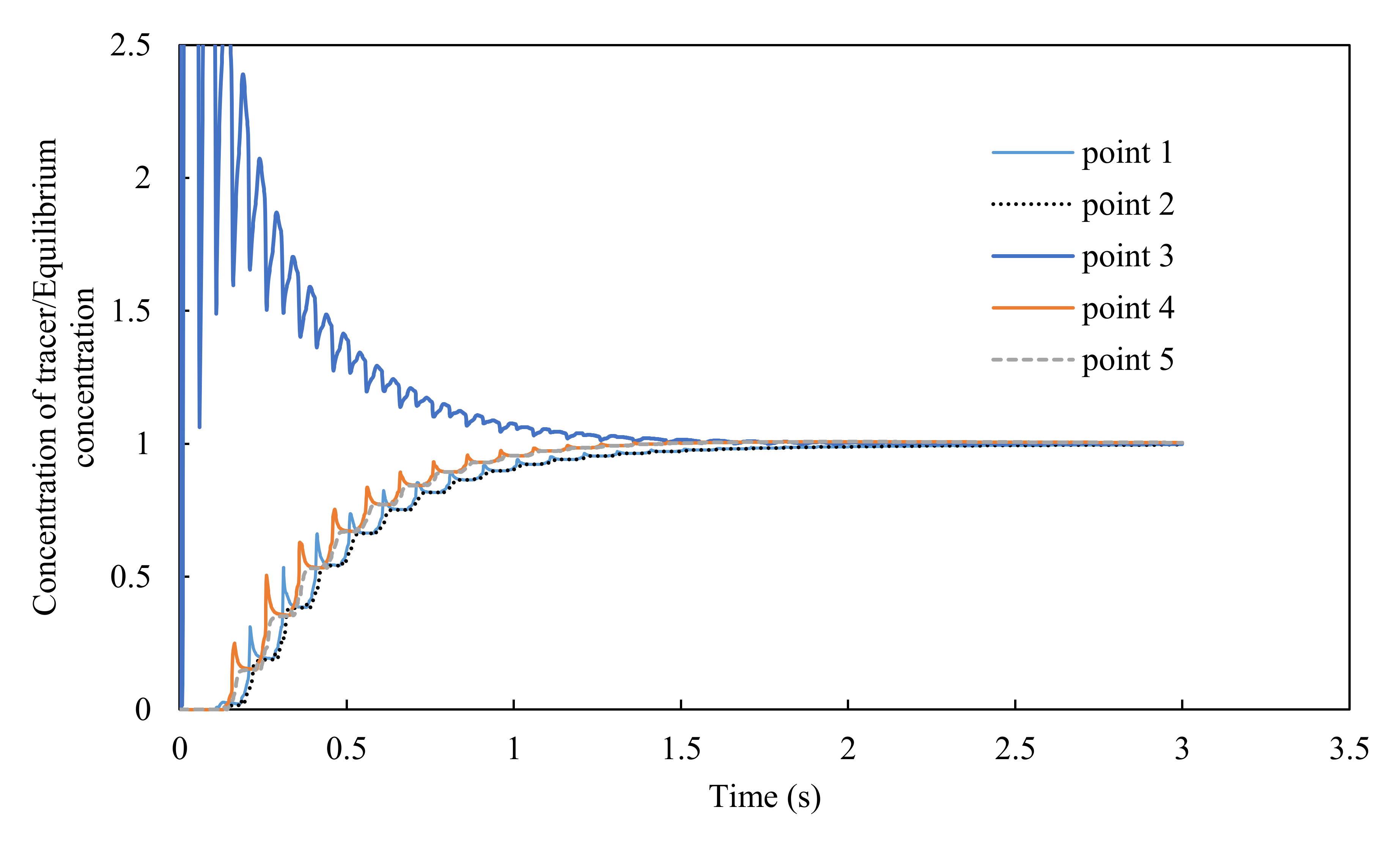
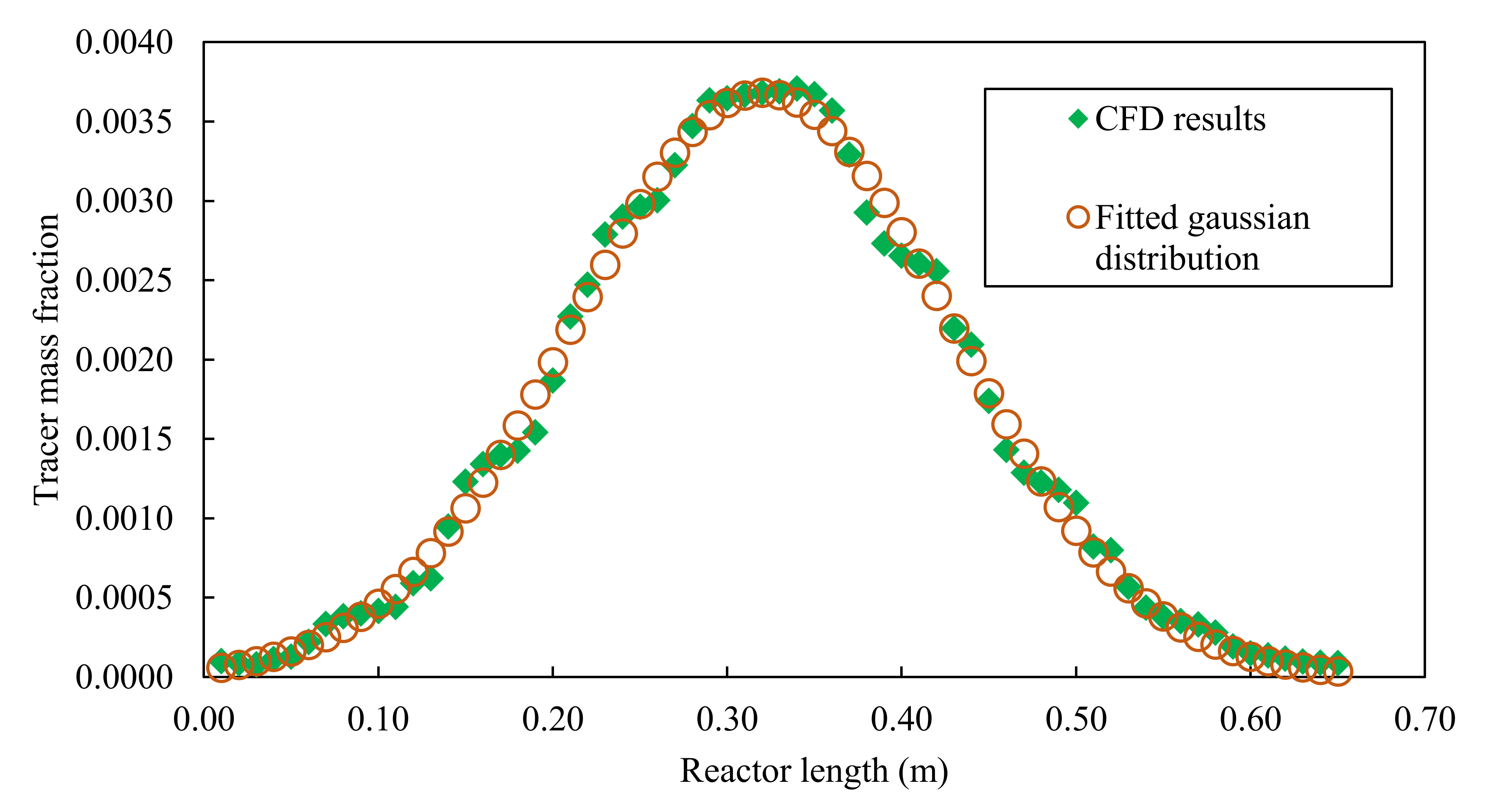
3.2. Mixing Time and Axial Dispersion Coefficient

Both the mixing time and axial dispersion coefficient require a tracer to be added to the system in order for their values to be obtained, whether in experimental work or a CFD model. For our study, 2.26 mg of a tracer (a fluid mass with the same viscosity and density as those of the working fluid) was patched into the entire center cross-section of the column and tracked using a species transport model.

Mixing time is the time needed for a system to reach a uniform equilibrium concentration after adding a certain amount of tracer [20]. To obtain that, five monitoring points (refer to Figure 1b) were specified where the concentration had been tracked along the time. The reason for choosing these points is that they were expected to be the last points where the concentration reached the equilibrium concentration ($C_{\infty })$.

We assumed a final deviation of ± 5% from $C_{\infty }$ to measure the mixing time, since the concentration approaches $C_{\infty }$ in an asymptotic and sinusoidal manner (Figure 8), which makes it difficult to find the moment that the concentration reaches the equilibrium concentration. $C_{\infty }$ can be calculated using the following equation.

$$V_{initial}{C}_{initial}+V_{injection}{C}_{injection}= V_{final}{C}_{\infty }$$

(28)

The mixing time for the points indicated in Figure 1b in different oscillation frequencies and amplitudes are listed in

Table 3. Mixing time (s) in different operating conditions and different points.

Operating Condition	Point 1	Point 2	Point 3	Point 4	Point 5	Maximum
40 mm of amplitude, 10 Hz of frequency	1.21	1.22	1.10	0.96	0.97	1.22
40 mm of amplitude, 9 Hz of frequency	1.33	1.35	1.23	1.16	1.17	1.35
40 mm of amplitude, 8 Hz of frequency	1.49	1.51	1.32	1.31	1.33	1.51
40 mm of amplitude, 2 Hz of frequency	5.45	5.53	6.91	8.67	8.74	8.74
40 mm of amplitude, 1.5 Hz of frequency	8.35	8.54	11.43	7.94	8.02	11.43
40 mm of amplitude, 1 Hz of frequency	15.03	16.73	13.02	16.52	15.65	16.73
30 mm of amplitude, 2 Hz of frequency	22.29	22.18	9.55	8.22	8.29	22.29
20 mm of amplitude, 2 Hz of frequency	26.07	23.56	19.68	14.29	15.84	26.07
8 mm of amplitude, 2 Hz of frequency	55.42	57.36	56.78	60.82	59.73	60.82
6 mm of amplitude, 2 Hz of frequency	61.68	68.19	54.66	76.17	69.67	76.17
4 mm of amplitude, 2 Hz of frequency	144.84	154.53	79.26	145.4	156.19	156.19

. In that table, the column “maximum” is the highest value among all the mixing times corresponding to each point and as expected, the mixing times at point 5 and point 2 was higher than those at points 4 and 1, respectively, since the points on the reactor center line were the closest ones to the orifices that flow passes through. However, the difference between mixing time for two points on the same cross-section (point 1 and 2) and (point 4 and 5) was so small in all oscillating conditions that it can be concluded that the flow inside a moving baffle OBR is uniform along the reactor radius. In addition, points 1 and 4 were expected to have the same values, as they were the same distance from the reactor centerline. However, one of them showed a higher or lower value, depending on in which direction the first stroke occurred.

The effect of oscillatory Reynolds number, oscillation amplitude, and oscillation frequency on mixing time is summarized in Figure 9, where the maximum mixing time was used for the plots. The mixing time decreased with the increase of oscillatory Reynolds number, oscillation frequency, and oscillation amplitude. In addition, low frequencies and oscillatory Reynolds number had more impact on the mixing time than high values of $R{e}_o$.

Mixing time is the most tangible mixing index; however, the issues associated with that parameter make it inappropriate for representing mixing performance. Firstly, mixing time has different values for different locations in the reactor, which is one of the disadvantages of using it. Finding the end point of the process is also a challenge as concentration asymptotically reaches its final value and, in our case, the concentration was fluctuating with fluid oscillation, which made it even more difficult to find the end point. In addition, it was computationally expensive to reach a uniform concentration throughout our system, especially for low frequencies and amplitudes.

Unlike mixing time, the axial dispersion coefficient is an index that can describe the mixing performance of both continuous and batch tubes. This parameter shows the deviation of flows from the ideal plug flow behavior in a continuous reactor or the rate at which a tracer spreads axially along a batch reactor length [50,51]. The axial dispersion coefficient has been also considered as a measure of macro-mixing (e.g., mechanical mixing of the bulk fluid) or micro-mixing (e.g., molecular diffusion) or usually a combination of both [51]. One of the advantages of the axial dispersion coefficient is that the residence time distribution of a continuous OBR can be obtained through this index. In addition, axial dispersion coefficients of batch and continuous reactors are almost equal in the same operating condition if the net Reynolds number is not greater than the oscillatory Reynolds number [51] and therefore, the value of the axial dispersion coefficient of batch and continuous OBRs can be used interchangeably. To calculate this index, either residence time distribution of an injected tracer for a continuous OBR or concentration profile of tracer of a batch OBR is required [50,51].

In our study, the method suggested by Manninen et al. [21] was used to obtain the axial dispersion coefficient. The one-dimensional convection–diffusion model for the tracer concentration ($c$) in tube flows was:

$$\frac{\partial c}{\partial t}=E\frac{{\partial }^{2}c}{\partial x^2}-u_{net}\frac{\partial c}{\partial t}$$

(29)

where E is the axial dispersion coefficient, $x$ is the axial coordinate, and $u_{net}$ is the mean axial fluid velocity in the column. Considering the absence of net flow in our batch OBR, the following equation (Equation (30)) was obtained, which is analogous to Fick’s law of molecular diffusion based on the assumption that the concentration is uniform along the reactor diameter.

$$\frac{\partial c}{\partial t}=E\frac{{\partial }^{2}c}{\partial x^2}$$

(30)

The solution of Equation (30) was the normal probability density function defined as:

$$c\left(x,t\right)=C_{tr}f\left(x|\theta ,\sigma \right)=\frac{C_{tr}}{\sigma \sqrt{2\pi }}{e}^{\frac{-{\left(x-\theta \right)}^2}{2{\sigma }^2}}$$

(31)

where the coefficient $C_{tr}$ is given by $C_{tr}=m_{tr}/A$; $m_{tr}$ is the mass of the tracer; $A$ is the cross-sectional area of the reactor; and $\theta$ is the mean value. The tracer concentration distribution along the reactor length was obtained by averaging the concentration at each cross-section distanced equally from each other to create a one-dimensional distribution. Figure 10 is an example of these distributions, which showed an almost Gaussian distribution at a specific instant of time. By fitting Equation (31) into the tracer concentration distribution, ${\sigma }^2$ and $\theta$ were obtained at each flow time. In an ideal case, ${\sigma }^2=Et$, where $t$ is the time at which the distribution is tracked after patching the tracer. However, in reality, it takes some time before the tracer concentration shows a Gaussian distribution. Therefore, we have ${\sigma }^2=E\left(t-t_0\right)$, where $t_0$ is the first time in which the tracer shows a Gaussian distribution along the reactor length. Hence, the axial distribution coefficient can be obtained by calculating the slope of ${\sigma }^2$ against $t$. By employing a different oscillation frequency and amplitude, the axial dispersion coefficient was plotted against an oscillatory Reynolds number, oscillation frequency, and oscillation amplitude, as illustrated in Figure 11.

It can be observed that the axial dispersion coefficient and oscillatory Reynolds number had an almost linear relationship with both low and high Reynolds numbers. This was expected, since the increase of oscillatory Reynolds number results in an increase in turbulence and thus an increase in fluid dispersion [1].

In addition, axial dispersion increased with the increase of either oscillation frequency or oscillation amplitude. However, the latter showed a more significant impact on axial dispersion. Besides, the oscillatory Reynolds number did not necessarily describe the reactor behavior, since there were two different axial dispersions for the same oscillatory Reynolds number, as can be seen in Figure 11. It also shows that high amplitudes had a stronger impact on axial dispersion than low amplitudes.

Another advantage of the axial dispersion coefficient is that it is independent of the location of concentration tracking and time. In addition, the index can describe an OBR better than the other aforementioned indices, which will be discussed in the following section.

3.3. Mixing Parameters Comparison

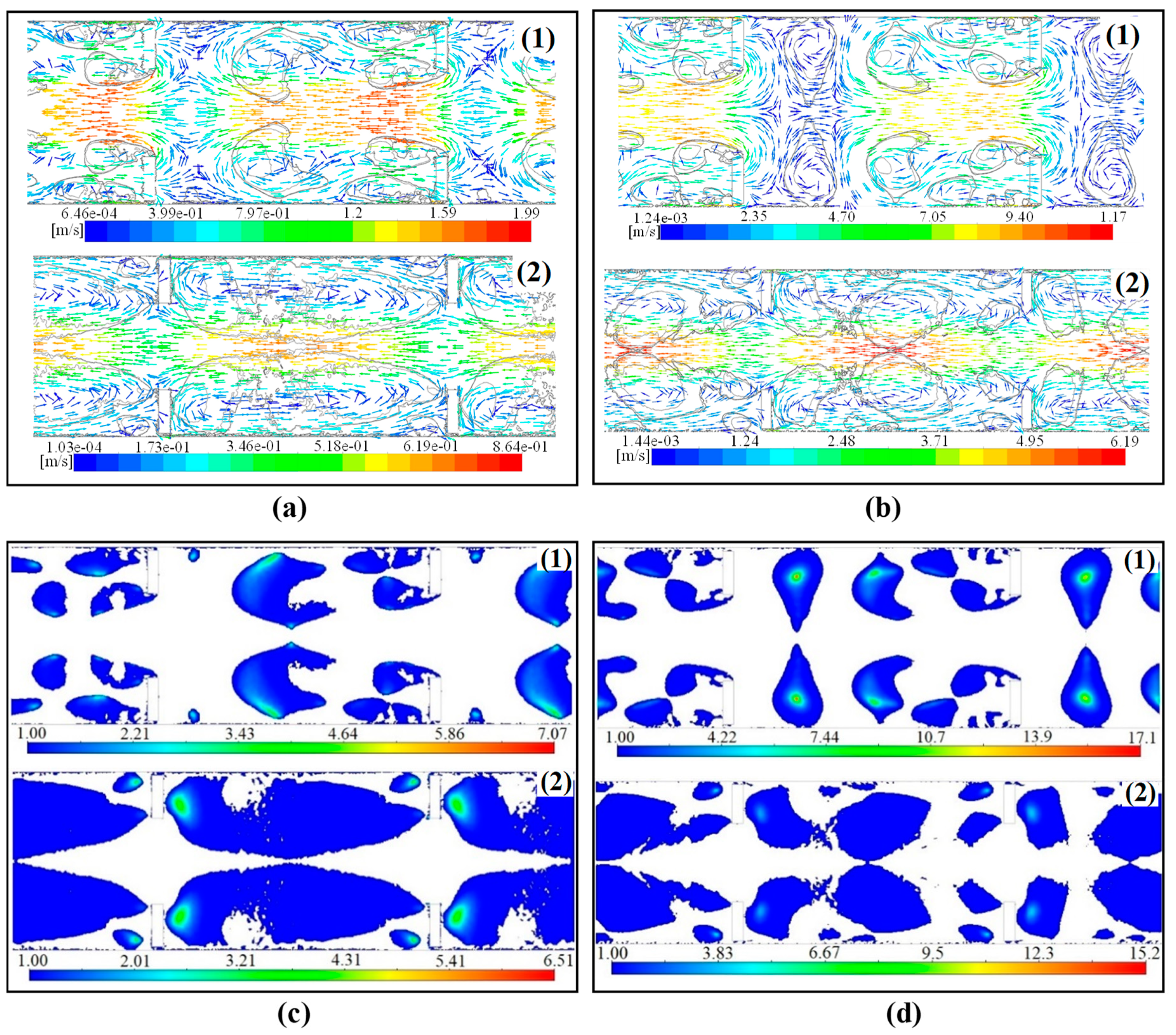
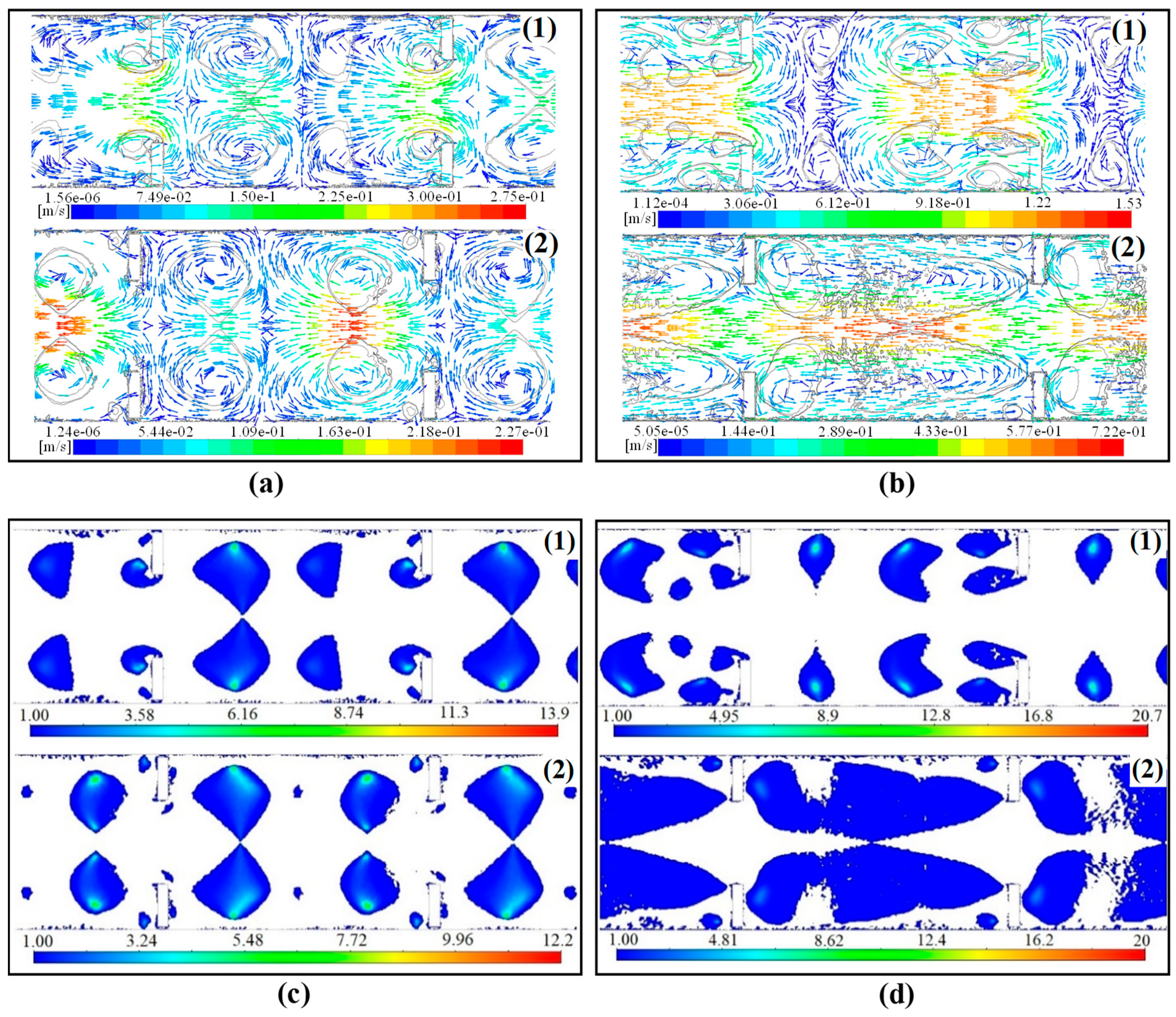
In the previous section, various mixing indices were introduced, and the effect of changing operating conditions on them was investigated. In this section, considering the aforementioned drawbacks associated with mixing time, we made a comparison among all the parameters mentioned above by taking mixing time as the basis for representing mixing performance, since this index is the most tangible one in quantifying mixing performance. The values of all the mixing indices are listed in

Table 4. The values of mixing indices in different operating conditions.

Operating Condition	Mixing Time (s)	Velocity Ratio	Turbulent Length Scale (m)	Turbulent Time Scale (s)	Axial Dispersion Coefficient (m2/s)
40 mm of amplitude, 10 Hz of frequency	1.21	4.024	0.00859	0.00029	0.0974
40 mm of amplitude, 9 Hz of frequency	1.33	4.004	0.00866	0.00033	0.0834
40 mm of amplitude, 8 Hz of frequency	1.49	4.003	0.00877	0.00040	0.0683
40 mm of amplitude, 2 Hz of frequency	5.45	3.887	0.01024	0.00287	0.0204
40 mm of amplitude, 1.5 Hz of frequency	8.35	3.831	0.01051	0.00423	0.0108
40 mm of amplitude, 1 Hz of frequency	15.03	3.719	0.01075	0.00732	0.0057
30 mm of amplitude, 2 Hz of frequency	22.29	3.606	0.01032	0.00399	0.0087
20 mm of amplitude, 2 Hz of frequency	26.07	3.038	0.01026	0.00638	0.0041
8 mm of amplitude, 2 Hz of frequency	55.42	1.938	0.01016	0.02022	0.0012
6 mm of amplitude, 2 Hz of frequency	61.68	1.798	0.00976	0.03036	0.0007
4 mm of amplitude, 2 Hz of frequency	144.84	1.659	0.00875	0.05651	0.0003

for every operating condition. For better comparison of these indices with mixing time, the logarithmic plots of velocity ratio, turbulent length scale, turbulent time scale, and axial dispersion coefficient versus mixing time was obtained and shown in Figure 12. These plots are useful, since they allow us to compare parameters with different trends against mixing time. If the relationship is linear, it means that the mixing parameter has a meaningful relationship with mixing time. Otherwise, it shows an uncorrelated relationship (Figure 12a,b), meaning that the parameter is not able to represent mixing time. This was expected, as the primary purpose of defining the velocity ratio and turbulent mixing length is not about quantifying the mixing performance of an OBR, which is explained in Section 3.1.

As shown in Figure 12, the value of squared regression for the natural logarithm of the axial dispersion coefficient and turbulent time scale was close to 1, meaning that the axial dispersion coefficient and turbulent time scale have a meaningful relationship with the mixing time, making them suitable candidates for mixing performance. However, the axial dispersion coefficient has the advantage of being obtained through both experimental and CFD approaches, while the turbulent time scale can only be calculated through CFD. The residence time distribution of a continuous OBR can be obtained through this index. In addition, axial dispersion coefficients of batch and continuous reactors are almost equal under the same operating condition if the net Reynolds number is not greater than the oscillatory Reynolds number [51]; therefore, the value of the axial dispersion coefficient of batch and continuous OBRs can be used interchangeably. Another advantage of the axial dispersion coefficient over the mixing time is that it needs much less time to be calculated. As an example, it takes 156.91 s (obtained after around 3 weeks of calculation time) for the OBR to reach equilibrium at 4 mm of amplitude and 2 Hz of frequency, while axial dispersion requires only 5 s (obtained after 2 days of calculation time) after adding the tracer to the system to be calculated at 40 mm of amplitude and 10 Hz of frequency. It means that the axial dispersion coefficient is less computationally expensive than the mixing time, and it can better represent the mixing time.

3.4. Hydrodynamics

In this section, the hydrodynamic behavior of the reactor under different conditions and phases of oscillation is discussed. All the contours and maps shown in this section present just one cell (the area between two adjacent baffles) instead of the entire reactor, since all the cells have similar velocity vector maps at each phase, except for the bottom and top cells, which only contain small volumes with respect to the whole OBR. Therefore, the different flow behavior in those regions can be neglected. To discuss the hydrodynamic parameters of this moving baffle OBR, phases 1 and 2 were selected from four oscillation phases, which are illustrated in Figure 13 due to the similarity of phase 1 with phase 3 and phase 2 with phase 4.

In order to compare the effect of oscillation frequency on the flow field of OBRs, two operating conditions (including one with $x_o$ = 40 mm and $f$ = 2 Hz and the other one with $x_o$ = 40 mm and $f$ = 10 Hz) were selected. To investigate the effect of oscillation amplitude, two other operating conditions were used, including one with $x_o$ = 6 mm and $f$ = 2 Hz and the other one with $x_o$ = 30 mm and $f$ = 2 Hz.

Figure 14a,b shows the velocity magnitude vector map along with Q-criterion iso-surfaces (black curves) for varying frequency comparison. Q-criterion, a parameter introduced by [52], was used to determine the vortices in our system and is defined as the square of the vorticity minus the square of the shear strain rate (Equation (32)) [4]. The vorticity ($\mathsf{\Omega }$) (Equation (33)), which is the curl of velocity, shows the magnitude of fluid rotation, and shear strain rate ($SSR$) (Equation (34)) represents the magnitude of fluid stretching. Thus, positive Q-criterion values mean a higher value of vorticity magnitude than that of the strain rate, which shows the region where fluid rotation is dominant over fluid stretching [53].

$$Q=\frac{1}{2}\left({\Vert \mathsf{\Omega }\Vert }^2-{\Vert SSR\Vert }^2\right)>0$$

(32)

$$\mathsf{\Omega }=\frac{1}{2}\left(\frac{\partial U_i}{\partial x}-\frac{\partial U_j}{\partial y}\right)$$

(33)

$$SSR=\frac{1}{2}\left(\frac{\partial U_i}{\partial x}+\frac{\partial U_j}{\partial y}\right)$$

(34)

In the above-mentioned equations $U_i$ and $U_j$ are the velocities in the $x$ and $y$ directions, respectively. The Q-criterion iso-surfaces created in Figure 14a,b and Figure 15a,b were the surfaces with the same parameter value, which can determine the core of vortices to a good extent. A modification on Q-criterion (Equation (35)) suggested by rearranging Equation (32) was used for determining the position of vortices.

$$modified Q=\frac{\Vert \mathsf{\Omega }\Vert }{\Vert SSR\Vert }>1$$

(35)

The contours of modified Q-criterion with values higher than 1 are illustrated in Figure 14c,d, and Figure 15c,d, which include different operating conditions (see the figure captions). Comparing the velocity vector maps and modified Q-criterion contours in Figure 14 and Figure 15, we found good agreement between the location of the vortices in the velocity vector map and the contour of the modified Q-criterion for each oscillation condition. In addition, the modified Q-criterion had a narrower range than that of the Q-criterion and was dimensionless, which is more desirable for further use in any possible correlation. Therefore, the suggested modified Q-criterion can be a viable replacement of Q-criterion for vortex identification.

As can be seen in Figure 14 (constant $x_o$ = 40 mm), for both oscillation conditions in phase 2, the flow passing through the orifices hardly interacted with the vortices formed within the inter-baffle area. However, in phase 1, there were vortices that had the diameter of the entire reactor diameter. Furthermore, the flow field maps look similar for both oscillation conditions at each phase. In other words, the number and the location of the vortices were more or less the same, despite some slight differences in the size of vortices. These are the main reasons why the oscillation frequency did not have a significant contribution to mixing performance while also showing why high amplitudes provided high mixing quality. We observed that vortices were closer to the wall for $f$ = 2 Hz than $f$ = 10 Hz, meaning that there was a slightly better axial dispersion for 10 Hz of frequency than for 2 Hz of frequency, which agrees with what is previously found in Section 3.2.

Figure 15 (constant $f$ = 2 Hz) demonstrated that the velocity vector maps for $x_o$ = 6 mm and $x_o$ = 30 mm were totally different. In $x_o$ = 6 mm, two large vortices with equal size can be seen that cover the entire column radius at every oscillation phase. However, in $x_o$ = 30 mm, the flow entering from one orifice is not involved in any formed vortex and goes directly to the next orifice. Therefore, it can be concluded that small amplitudes were not able to break the formed vortices, and this is the most important reason behind the significance of oscillation amplitude in the mixing performance of an OBR.

As a general assessment of flow behavior in an OBR, in high oscillation amplitudes (>20 mm), there is only one large vortex extending from one baffle to another with several tiny vortices formed around the wall and the baffles, while a main stream going directly form one orifice to another does not heavily involve vortices for the large part of oscillation cycle. Under low amplitudes (<8 mm), two almost equal-size vortices are formed along the reactor radius, which remain unchanged during the oscillation cycle. By comparing the velocity vector maps and modified Q-criterion contours in Figure 14 and Figure 15, we found that the modified Q-criterion can be useful for determining the location and the size of vortices for a moving baffle OBR. Further studies are needed to see how the modified Q-criterion performs for determining vortices in different systems.

Shear Strain Rate

Figure 16 and Figure 17 show the impact of different oscillation frequencies and amplitudes on the shear strain rate ($SSR$). This is important to know, since OBRs have attracted attention for performing bioprocesses and emulsions that can include shear-sensitive cells and particles. Studies have shown that OBR can be an alternative for performing bioprocesses that are inhibited by the high shear strain rate generated in STRs where a specific degree of mixing is required to achieve sufficient mass transfer. However, no information can be found on the shear strain rate of a moving baffle OBR in the literature. Similar to Figure 14 and Figure 15, oscillation phases 1 and 2 are shown in Figure 16 to investigate the effect of oscillation frequency and oscillation amplitude on $SSR$ contour. It can be seen that $SSR$ had the highest value in the regions closest to the baffles, especially around the edges, regardless of the oscillation frequency, oscillation amplitude, and phase of oscillation. Considering that the regions with a high shear rate have a small volume compared to the whole reactor, it can be concluded that the shear rate was uniform throughout the reactor at any moment over an oscillation cycle. The uniformity of shear rate is an important property of moving baffle OBRs that make them suitable for bioprocesses especially where larger particles, millimeters in size, are being used [5].

According to Figure 17 which shows the average $SSR$ over an oscillation cycle against the operating conditions, $SSR$ had an almost perfectly linear relationship with oscillation frequency, oscillation amplitude, and oscillatory Reynolds number. $SSR$ equations as a function of f, $x_o$, and $R{e}_o$ with corresponding square regression values can also be seen in Figure 17. It can be concluded that the oscillatory Reynolds number can be a perfect tool for predicting the time average $SSR$ in a moving baffle OBR. This is completely opposite to the behavior of unpredictable mixing parameters by having the value of $R{e}_o$. Considering that increasing $R{e}_o$ improves the mixing performance and increases $SSR$, which is not desirable, an optimum value for $R{e}_o$ has to be found for bioprocesses, which can be the subject of future research.

4. Conclusions

A comprehensive study on the mixing performance and hydrodynamics of a moving baffle OBR was performed using different mixing indices after validating a CFD model with experimental data. Dynamic mesh proved to be a successful tool to model moving baffle OBR, which had not been used thus far. The effects of oscillatory Reynolds number, oscillation frequency, and oscillation amplitude on the mixing indices were tested. It was determined that the oscillation amplitude had a more significant impact on the mixing performance than the oscillation frequency. In addition, it was found that the mixing indices did not necessarily show similar behavior in high and low values. For instance, the mixing time decreased with a higher slope in low $R{e}_o$s than with high $R{e}_o$s. The oscillatory Reynolds number did not describe the reactor behavior, as there were different values of each mixing index in a single oscillatory Reynolds number.

The axial dispersion coefficient provided the most accurate alternative to mixing time while also not having the disadvantages of the mixing time (dependence on the location of concentration detection and the equilibrium concentration). In addition, to obtain the axial dispersion coefficient, it is not necessary for the tracer to reach equilibrium concentration, which is especially important when CFD is employed. However, the need to present a new index for quantifying the mixing performance in a moving baffle OBR still exists due to the difficulties of calculating the axial dispersion coefficient. One of those difficulties includes obtaining tracer size distribution along the reactor length, especially through experimental methods.

The hydrodynamic behavior of our reactor was investigated using the velocity vector, Q-criterion, and $SSR$. A rearrangement on the correlation of the Q-criterion resulted in a new criterion that not only performed well in determining the location and the size of vortices but also offered a narrower range of values in an oscillation period compared to the Q-criterion. The new criterion is dimensionless, which makes it desirable for developing new dimensionless correlations. Finally, $SSR$ was found to be uniform throughout the reactor at any instance during the oscillation cycle, and a linear correlation between $SSR$ and $R{e}_o$ was obtained that showed the predictability of $SSR$ in a moving baffle OBR. This information on $SSR$ is very important, especially in bioprocesses, due to the presence of shear-sensitive materials. All in all, a correlation for $SSR$ and an appropriate mixing index, i.e., an axial dispersion coefficient, provides a suitable design platform for a moving baffle OBR. However, there are still other important parameters such as power consumption, particle size distribution, etc., which need to be studied for a comprehensive design of a moving baffle OBR.

References

1. Ni, X.; Pereira, N.E. Parameters affecting fluid dispersion in a continuous oscillatory baffled tube. Aiche J. 2000, 46, 37–45. [Google Scholar] [CrossRef]
2. McGlone, T.; Briggs, N.E.; Clark, C.A.; Brown, C.J.; Sefcik, J.; Florence, A.J. Oscillatory flow reactors (OFRs) for continuous manufacturing and crystallization. Org. Process Res. Dev. 2015, 19, 1186–1202. [Google Scholar] [CrossRef] [Green Version]
3. Van Dijck, W.J.D. Process and Apparatus for Intimately Contacting Fluids; United States Patent Office: Washington, DC, USA, 1935. [Google Scholar]
4. Mazubert, A.; Fletcher, D.F.; Poux, M.; Aubin, J. Hydrodynamics and mixing in continuous oscillatory flow reactors—Part I: Effect of baffle geometry. Chem. Eng. Process. Process Intensif. 2016, 108, 78–92. [Google Scholar] [CrossRef]
5. Abbott, M.S.R.; Harvey, A.P.; Perez, G.V.; Theodorou, M.K. Biological processing in oscillatory baffled reactors: Operation, advantages and potential. Interface Focus. 2013, 3, 20120036. [Google Scholar] [CrossRef] [Green Version]
6. Ni, X.; Gough, P. On the discussion of the dimensionless groups governing oscillatory flow in a baffled tube. Chem. Eng. Sci. 1997, 52, 3209–3212. [Google Scholar] [CrossRef]
7. Jimeno, G.; Lee, Y.C.; Ni, X.W. On the evaluation of power density models for oscillatory baffled reactors using CFD. Chem. Eng. Process. Process Intensif. 2018, 134, 153–162. [Google Scholar] [CrossRef]
8. Laybourn, A.; López-Fernández, A.M.; Thomas-Hillman, I.; Katrib, J.; Lewis, W.; Dodds, C.; Harvey, A.P.; Kingman, S.W. Combining continuous flow oscillatory baffled reactors and microwave heating: Process intensification and accelerated synthesis of metal-organic frameworks. Chem. Eng. J. 2019, 356, 170–177. [Google Scholar] [CrossRef] [Green Version]
9. Smith, K.B. Scale-Up of Oscillatory Flow Mixing. Ph.D. Thesis, University of Cambridge, Cambridge, UK.
10. Jian, H.; Ni, X. A numerical study on the scale-up behaviour in oscillatory baffled columns. Chem. Eng. Res. Des. 2005, 83, 1163–1170. [Google Scholar] [CrossRef]
11. Smith, K.B.; Mackley, M.R. An experimental investigation into the scale-up of oscillatory flow mixing in baffled tubes. Chem. Eng. Res. Des. 2006, 84, 1001–1011. [Google Scholar] [CrossRef] [Green Version]
12. Anderson, C.J.; Harris, M.C.; Deglon, D.A. Flotation in a novel oscillatory baffled column. Miner. Eng. 2009, 22, 1079–1087. [Google Scholar] [CrossRef] [Green Version]
13. Ni, X.; Cosgrove, J.A.; Arnott, A.D.; Greated, C.A.; Cumming, R.H. On the measurement of strain rate in an oscillatory baffled column using particle image velocimetry. Chem. Eng. Sci. 2000, 55, 3195–3208. [Google Scholar] [CrossRef]
14. Hewgill, M.R.; Mackley, M.R.; Pandit, A.B.; Pannu, S.S. Enhancement of gas-liquid mass transfer using oscillatory flow in a baffled tube. Chem. Eng. Sci. 1993, 48, 799–809. [Google Scholar] [CrossRef]
15. Ni, X.; Gao, S.; Cumming, R.H.; Pritchard, D.W. A comparative study of mass transfer in yeast for a batch pulsed baffled bioreactor and a stirred tank fermenter. Chem. Eng. Sci. 1995, 50, 2127–2136. [Google Scholar] [CrossRef]
16. Fitch, A.W.; Jian, H.; Ni, X. An investigation of the effect of viscosity on mixing in an oscillatory baffled column using digital particle image velocimetry and computational fluid dynamics simulation. Chem. Eng. J. 2005, 112, 197–210. [Google Scholar] [CrossRef]
17. Ni, X.; Stevenson, C.C. On the effect of gap size between baffle outer diameter and tube inner diameter on the mixing characteristics in an oscillatory-baffled column. J. Chem. Technol. Biotechnol. Int. Res. Process Environ. Clean Technol. 1999, 74, 587–593. [Google Scholar] [CrossRef]
18. Reis, N.; Vicente, A.A.; Teixeira, J.A.; Mackley, M.R. Residence times and mixing of a novel continuous oscillatory flow screening reactor. Chem. Eng. Sci. 2004, 59, 4967–4974. [Google Scholar] [CrossRef] [Green Version]
19. Stonestreet, P.; Harvey, A.P. A mixing-based design methodology for continuous oscillatory flow reactors. Chem. Eng. Res. Des. 2002, 80, 31–44. [Google Scholar] [CrossRef]
20. Ni, X.; Brogan, G.; Struthers, A.; Bennett, D.C.; Wilson, S.F. A systematic study of the effect of geometrical parameters on mixing time in oscillatory baffled columns. Chem. Eng. Res. Des. 1998, 76, 635–642. [Google Scholar] [CrossRef]
21. Manninen, M.; Gorshkova, E.; Immonen, K.; Ni, X.W. Evaluation of axial dispersion and mixing performance in oscillatory baffled reactors using CFD. J. Chem. Technol. Biotechnol. 2013, 88, 553–562. [Google Scholar] [CrossRef]
22. Gough, P.; Ni, X.; Symes, K.C. Experimental flow visualisation in a modified pulsed baffled reactor. J. Chem. Technol. Biotechnol. Int. Res. Process Environ. Clean Technol. 1997, 69, 321–328. [Google Scholar] [CrossRef]
23. Navarro-Fuentes, F.; Keane, M.; Ni, X.W. A Comparative Evaluation of Hydrogenation of 3-Butyn-2-ol over Pd/Al2O3 in an Oscillatory Baffled Reactor and a Commercial Parr Reactor. Org. Process Res. Dev. 2018, 23, 38–44. [Google Scholar] [CrossRef]
24. Ismail, L.; Westacott, R.E.; Ni, X. On the effect of wax content on paraffin wax deposition in a batch oscillatory baffled tube apparatus. Chem. Eng. J. 2008, 137, 205–213. [Google Scholar] [CrossRef]
25. Ni, X.; Johnstone, J.C.; Symes, K.C.; Grey, B.D.; Bennett, D.C. Suspension polymerization of acrylamide in an oscillatory baffled reactor: From drops to particles. Aiche J. 2001, 47, 1746–1757. [Google Scholar] [CrossRef]
26. Sutherland, K.; Pakzad, L.; Fatehi, P. CFD population balance modeling and dimensionless group analysis of a multiphase oscillatory baffled column (OBC) using moving overset meshes. Chem. Eng. Sci. 2019, 199, 552–570. [Google Scholar] [CrossRef]
27. Sutherland, K.; Pakzad, L.; Fatehi, P. Oscillatory power number, power density model, and effect of restriction size for a moving-baffle oscillatory baffled column using CFD modelling. Can. J. Chem. Eng. 2020, 98, 1172–1190. [Google Scholar] [CrossRef]
28. Falcucci, G.; Succi, S.; Montessori, A.; Melchionna, S.; Prestininzi, P.; Barroo, C.; Bell, D.C.; Biener, M.M.; Biener, J.; Zugic, B.; et al. Mapping reactive flow patterns in monolithic nanoporous catalysts. Microfluid. Nanofluidics. 2016, 20, 105. [Google Scholar] [CrossRef]
29. Montessori, A.; Prestininzi, P.; La Rocca, M.; Falcucci, G.; Succi, S.; Kaxiras, E. Effects of Knudsen diffusivity on the effective reactivity of nanoporous catalyst media. J. Comput. Sci. 2016, 17, 377–383. [Google Scholar] [CrossRef] [Green Version]
30. Ni, X.; Mackley, M.R.; Harvey, A.P.; Stonestreet, P.; Baird, M.H.I.; Rao, N.R. Mixing through oscillations and pulsations—A guide to achieving process enhancements in the chemical and process industries. Chem. Eng. Res. Des. 2003, 81, 373–383. [Google Scholar] [CrossRef]
31. Ni, X.W.; Fitch, A.; Jian, H. Numerical and experimental investigations into the effect of gap between baffle and wall on mixing in an oscillatory baffled column. Int. J. Chem. React. Eng. 2004, 2, 1–16. [Google Scholar] [CrossRef]
32. Howes, T.; Mackley, M.R.; Roberts, E.P.L. The simulation of chaotic mixing and dispersion for periodic flows in baffled channels. Chem. Eng. Sci. 1991, 46, 1669–1677. [Google Scholar] [CrossRef]
33. Mackley, M.R.; Tweddle, G.M.; Wyatt, I.D. Experimental heat transfer measurements for pulsatile flow in baffled tubes. Chem. Eng. Sci. 1990, 45, 1237–1242. [Google Scholar] [CrossRef]
34. Reis, N.; Harvey, A.P.; Mackley, M.R.; Vicente, A.A.; Teixeira, J.A. Fluid mechanics and design aspects of a novel oscillatory flow screening mesoreactor. Chem. Eng. Res. Des. 2005, 83, 357–371. [Google Scholar] [CrossRef] [Green Version]
35. Courant, R.; Friedrichs, K.; Lewy, H. Über die partiellen Differenzengleichungen der mathematischen Physik. Math. Ann. 1928, 100, 32–74. [Google Scholar] [CrossRef]
36. ANSYS. ANSYS Fluent Theory Guide; ANSYS, Inc.: Canonsburg, PA, USA, 2019. [Google Scholar]
37. Shao, W.; Cui, Z.; Wang, N.; Cheng, L. Numerical simulation of heat transfer process in cement grate cooler based on dynamic mesh technique. Sci. China Technol. Sci. 2016, 59, 1065–1070. [Google Scholar] [CrossRef]
38. Basha, N.; Kovacevic, A.; Rane, S. User defined nodal displacement of numerical mesh for analysis of screw machines in Fluent. In IOP Conference Series: Materials Science and Engineering; IOP Publishing: Bristol, UK, 2019; Volume 604, p. 012012. [Google Scholar]
39. Zhu, Q.; Zhang, Y.; Zhu, D. Study on dynamic characteristics of the bladder fluid pulsation attenuator based on dynamic mesh technology. J. Mech. Sci. Technol. 2019, 33, 1159–1168. [Google Scholar] [CrossRef]
40. Harvey, A.P.; Mackley, M.R.; Stonestreet, P. Operation and optimization of an oscillatory flow continuous reactor. Ind. Eng. Chem. Res. 2001, 40, 5371–5377. [Google Scholar] [CrossRef]
41. Jahoda, M.; Tomášková, L.; Moštěk, M. CFD prediction of liquid homogenisation in a gas–liquid stirred tank. Chem. Eng. Res. Des. 2009, 87, 460–467. [Google Scholar] [CrossRef]
42. Ekambara, K.; Dhotre, M.T. Simulation of oscillatory baffled column: CFD and population balance. Chem. Eng. Sci. 2007, 62, 7205–7213. [Google Scholar] [CrossRef]
43. Yakhot, V.; Orszag, S.A.; Thangam, S.; Gatski, T.B.; Speziale, C.G. Development of turbulence models for shear flows by a double expansion technique. Phys. Fluids A Fluid Dyn. 1992, 4, 1510–1520. [Google Scholar] [CrossRef] [Green Version]
44. Randolph, A.D.; Larson, M.A. Theory of Particulate Processes: Analysis and Techniques of Continuous Crystallization; Academic Press: Cambridge, MA, USA, 1971. [Google Scholar]
45. Luo, H.; Svendsen, H.F. Theoretical model for drop and bubble breakup in turbulent dispersions. Aiche J. 1996, 42, 1225–1233. [Google Scholar] [CrossRef]
46. Lister, J.D.; Smit, D.J.; Hounslow, M.J. Adjustable discretized population balance for growth and aggregation. Aiche J. 1995, 41, 591–603. [Google Scholar] [CrossRef]
47. Roudsari, S.F. Experimental and CFD Investigation of the Mixing of MMA Emulsion Polymerization in a Stirred Tank Reactor. Ph.D. Thesis, Ryerson University, Toronto, ON, Canada, 2015. [Google Scholar]
48. Agahzamin, S.; Pakzad, L. A comprehensive CFD study on the effect of dense vertical internals on the hydrodynamics and population balance model in bubble columns. Chem. Eng. Sci. 2019, 193, 421–435. [Google Scholar] [CrossRef]
49. McDonough, J.R.; Oates, M.F.; Law, R.; Harvey, A.P. Micromixing in oscillatory baffled flows. Chem. Eng. J. 2019, 361, 508–518. [Google Scholar] [CrossRef]
50. Fitch, A.W.; Ni, X. On the determination of axial dispersion coefficient in a batch oscillatory baffled column using laser induced fluorescence. Chem. Eng. J. 2003, 92, 243–253. [Google Scholar] [CrossRef]
51. Ni, X.; De Gélicourt, Y.S.; Baird, M.H.; Rao, N.V.R. Scale-up of single phase axial dispersion coefficients in batch and continuous oscillatory baffled tubes. Can. J. Chem. Eng. 2001, 79, 444–448. [Google Scholar] [CrossRef]
52. Hunt, J.C.; Wray, A.A.; Moin, P. Eddies, Stream, and Convergence Zones in Turbulent Flows. Stud. Turbul. Using Numer. Simul. Databases 1988, 2, 193–208. [Google Scholar]
53. Kolář, V. Vortex identification: New requirements and limitations. Int. J. Heat Fluid Flow 2007, 28, 638–652. [Google Scholar] [CrossRef]
Figure 1. (a) Schematic of the moving baffle oscillatory baffled reactor (OBR) [25], (b) modified geometry used for modeling (Points 1 to 5 are used for measuring the mixing time, which will be explained in Section 3.2), and (c) image of the mesh created (one cell (inter-baffle zone) is shown).
Processes 08 01236 g001
Figure 2. Dimensionless velocity magnitude ( V / 2 π f x o ) of the flow at the center point of the reactor over the time (t/τ) (oscillation frequency = 2 Hz and oscillation amplitude = 40 mm).
Processes 08 01236 g002
Figure 3. Comparison of cumulative droplet size distribution for computational fluid dynamics (CFD) results with experimental data using Eulerian and Mixture multiphase models.
Processes 08 01236 g003
Figure 4. Radial velocity profile as a function of radius at x = 327 mm (centerline of the reactor) for 40 mm of oscillation amplitude and 2 Hz of oscillation frequency.
Processes 08 01236 g004
Figure 5. Velocity ratio versus (a) oscillatory Reynolds number, (b) oscillation frequency, and (c) oscillation amplitude.
Processes 08 01236 g005
Figure 6. Velocity ratio vs. dimensionless oscillation time (t/τ) for different oscillation conditions indicated above each plot.
Processes 08 01236 g006
Figure 7. Turbulent length scale versus (a) oscillatory Reynolds number, (b) oscillation frequency, and (c) oscillation amplitude and turbulent time scale versus, (d) oscillatory Reynolds number, (e) oscillation frequency, and (f) oscillation amplitude.
Processes 08 01236 g007
Figure 8. The ratio of the concentration of the tracer to equilibrium concentration against time in points 1 to 5 (oscillation frequency = 10 Hz, oscillation amplitude = 40 mm).
Processes 08 01236 g008
Figure 9. Mixing time versus (a) oscillatory Reynolds number, (b) oscillation frequency, (c) oscillation amplitude.
Processes 08 01236 g009
Figure 10. Axial distribution of tracer concentration in t = 1s for 40 mm of oscillation amplitude and 2 Hz of oscillation frequency.
Processes 08 01236 g010
Figure 11. Axial dispersion coefficient versus (a) oscillatory Reynolds number, (b) oscillation frequency, and (c) oscillation amplitude.
Processes 08 01236 g011
Figure 12. Natural logarithm of (a) velocity ratio, (b) turbulent length scale, (c) turbulent time scale, and (d) axial dispersion coefficient vs. natural logarithm of mixing time.
Processes 08 01236 g012
Figure 13. Oscillations phases during an oscillation cycle.
Processes 08 01236 g013
Figure 14. (a) Velocity vector map for f = 2 Hz and x o = 40 mm, (b) velocity vector map for f = 10 Hz and x o = 40 mm, (c) modified Q-criterion contour for f = 2 Hz and x o = 40 mm, (d) modified Q-criterion contour for f = 10 Hz and x o = 40 mm (different phases of the oscillation cycle are shown in top corner of each plot).
Processes 08 01236 g014
Figure 15. (a) Velocity vector map for f = 2 Hz and x o = 6 mm, (b) velocity vector map for f = 2 Hz and x o = 30 mm, (c) modified Q-criterion contour for f = 2 Hz and x o = 6 mm, (d) modified Q-criterion contour for f = 2 Hz and x o = 30 mm (different phases of oscillation cycle are shown in the top corner of each plot).
Processes 08 01236 g015
Figure 16. Shear strain rate contour for (a) f = 2 Hz and x o = 40 mm, (b) f = 10 Hz and x o = 40 mm, (c) f = 2 Hz and x o = 6 mm, (d) f = 2 Hz and x o = 30 mm (the different phases of the oscillation cycle are shown in the top corner of each plot).
Processes 08 01236 g016
Figure 17. Shear strain rate versus (a) oscillatory Reynolds number, (b) oscillation frequency, and (c) oscillation amplitude.
Processes 08 01236 g017