Coarse-Grain DEM Modelling in Fluidized Bed Simulation: A Review

Abstract

In the last decade, a few of the early attempts to bring CFD-DEM of fluidized beds beyond the limits of small, lab-scale units to larger scale systems have become popular. The simulation capabilities of the Discrete Element Method in multiphase flow and fluidized beds have largely benefitted by the improvements offered by coarse graining approaches. In fact, the number of real particles that can be simulated increases to the point that pilot-scale and some industrially relevant systems become approachable. Methodologically, coarse graining procedures have been introduced by various groups, resting on different physical backgrounds. The present review collects the most relevant contributions, critically proposing them within a unique, consistent framework for the derivations and nomenclature. Scaling for the contact forces, with the linear and Hertz-based approaches, for the hydrodynamic and cohesive forces is illustrated and discussed. The orders of magnitude computational savings are quantified as a function of the coarse graining degree. An overview of the recent applications in bubbling, spouted beds and circulating fluidized bed reactors is presented. Finally, new scaling, recent extensions and promising future directions are discussed in perspective. In addition to providing a compact compendium of the essential aspects, the review aims at stimulating further efforts in this promising field.

1. Introduction

The fluidized bed technology is at the very heart of a very broad number of industrial processes, ranging from chemical transformations in reactors (energy conversion and storage, (bio-)oil refining, chemical synthesis, polymerization) to physical operations (solids mixing or separation, drying, coating, agglomeration) [1]. Specialized applications can be found in the development of bioartificial organs [2,3].

Modelling of the gas- and liquid-solid flow in fluidized beds has traditionally relied on the similarity of the fluidized solid motion with a pseudo-liquid phase, through the concept of a gas-solid suspension. Even from a lexical point of view, the terms “fluidization”, “bubbling”, “emulsion phase”, “floating” and “sinking” of objects in the suspended particle bed recall the behavior of liquids. Based on this idea, the Two-Fluid Model (TFM) concept [4] was introduced, complemented by the kinetic theory of granular flow (KTGF), giving rise to groundbreaking success in the simulation of large-scale systems, as summarized in the book by Gidaspow [5]. At the other extreme, i.e., the small-scale interaction between the fluid and individual particles, discrete-continuum (or Eulerian-Lagrangian) simulations based on the discrete element method appeared, thanks to the progress in the computational power, giving rise to the CFD-DEM (Computational Fluid Dynamics-Discrete Element Method) approach [6]. The recognition of the discrete nature of the granular medium proved to be a key ingredient and allowed important new features of fluidized systems to be captured, as discussed in several reviews (e.g., [7,8,9,10,11,12]).

The most significant drawback of CFD-DEM is the feasibility of realistic simulations, as the combination of practical sizes, number of particles and required time to simulate very quickly saturates the computing capability of the most powerful supercomputer. As examples of the achievable scale in terms of numbers of particles, CFD-DEM simulations reached 4.5 million particles in bubbling beds [13] and up to 25 million particles using the power of the GPU [14]. In a recent review on methods for granular and particle-fluid flow, with focus on strategies for engineering applications, Ge et al. [15] noted that the typical time step is 10⁻⁵–10⁻⁶ s and an engineering system may contain 10⁸–10¹² particles, with characteristic flow or transport time ranges of 10¹–10⁴ s (see also [14]). The necessary time and hardware resources to perform direct DEM simulations and post-process the results of such systems are prohibitively costly and hence they remain infeasible.

In the last years, the push to save CPU time while maintaining the discrete nature of the simulated elements has been a very strong driver for novel strategies and methods. From the physical point of view, Lu et al. [16] noted that in most fluidized bed applications, only the collective behavior of the particles is of primary interest, rather than their individual trajectories. This forms the basis of practical demand for the application of coarse-graining to DEM. The idea behind coarse-grained DEM (or CG-DEM) is to substitute the actual particles by a smaller number of representative elements, whose behavior shall be equivalent in full to the original ones. These representative particles, often called “parcels”, become the elements whose motion is tracked by the simulations. They are not required to exist in reality, but their study provides useful data and insight on the real system they represent. The concept of parcels is very common in the context of the MP-PIC method, another Eulerian-Lagrangian technique which falls between TFM and CFD-DEM; the main difference is that solid stresses are treated by indirect models rather than explicitly like in DEM.

Previous attempts to modify the contact parameters to speed up DEM simulations is extremely common for particulate systems in the collisional or dilute regime. At the risk of introducing artifacts, some authors investigated different model laws to speed up the simulation; see e.g., [17]. In the coarse graining method, the objective is to scale size and parameters, and adapt models, so that the properties at the scale of the represented particles are kept constant. Among the early ideas of coarse-grained DEM, the following approaches can be mentioned: the imaginary sphere model [18], Similar Particle Assembly [19,20], Representative Particle Model [21]; the work of Patankar and Joseph [22], in which one model of the Lagrange treatment of the solid phase is based on a parcel-like DEM model, deserves to be mentioned. The two CG-DEM models that found widespread adoptions were proposed by Sakai et al. [23] for pneumatic conveying and by Bierwisch et al. [24] in the context of simulation of the cavity filling process. In the same period, Radl et al. [25] proposed scaling rules for parcels in dense gas-particle flows and Hilton and Cleary [26,27] showed an application to fluidized beds. The idea of using scaling rules to save on computational time was also tested [28], with limited success, as with exact scaling the simulation speed-up came at the cost of longer times to simulate, frustrating the ambitions of the method. Other interesting results related to similarity and simulations are found in [29,30,31]. Overall, application of the coarse graining method to DEM simulations is attracting a quickly growing attention in recent times, as shown by the yearly number of papers on the subject (see Figure 1). Early applications have been reported in commercial software packages [32] and are available in recent versions, see e.g., [33,34,35]. The feature is available also in the last version (20.4) of the open-source software MFiX-DEM [36].

The present contribution aims at critically reviewing the work done so far, presenting the approaches that found widespread adoption within a consistent and coherent framework, occasionally comparing the formulations; quantifying the theoretical computational savings as well as discussing the most critical issues affecting accuracy and reliability; presenting a picture of the state-of-the-art and finally discussing the most recent extensions and the questions still open.

A final introductory note to the reader: One should be aware that the topics covered here do not include other methods incidentally also known as “coarse graining” in DEM, which are used to migrate quantities from the micro- to the macroscale (like e.g., [37]) or smoothing discrete quantities for coupling ([38]).

2. Conventional Approach

2.1. CFD-DEM Modelling for Fluidized Beds

In CFD-DEM, the equations governing the two phases are solved separately, i.e., sequentially. Since the characteristic times can be different, distinct time-steps are used for the CFD and the DEM parts, so that generally the fluid flow remains constant for a number of DEM (smaller) time-steps.

The fluid phase flow is solved by a locally averaged approximation of the continuity and Navier–Stokes equations. The velocity and pressure fields are obtained by numerically integrating the following set of differential equations:

$$\frac{\partial \epsilon {\rho }_f}{\partial t}+\nabla \cdot \left(\epsilon {\rho }_f\mathit{u}\right)=0$$

(1)

$$\frac{\partial \epsilon {\rho }_f\mathit{u}}{\partial t}+\nabla ·\left(\epsilon {\rho }_f\mathit{u}\mathit{u}\right)=-\nabla p+\nabla ·\mathit{\tau }+{\mathit{F}}_{fp}+\epsilon {\rho }_f\mathit{g}$$

(2)

where ${\mathit{F}}_{fp}$ represents the interphase momentum transfer per unit volume between the particles and the fluid. The full system is closed with the definition of such term, which in our formulation reads:

$${\mathit{F}}_{fp}=-\frac{{\sum }_i^{N_p}{w}_i\left({\mathit{F}}_{d,i}+{\mathit{F}}_{b,i}\right)}{\Psi },$$

(3)

in which $N_p$ is the number of particles in the volume $\Psi$; the forces $F_d$ and $F_b$ represent the drag and pressure gradient (or generalized buoyancy) force, respectively; and $w_i$ is a weight function evaluated at the particle center, which allows the resulting source term in Equation (2) to be smoothed out over grid cells.

Our simulations are based on a modelling approach combining the Discrete Element Method for the solid phase and a local average CFD approach for the fluid phase. The physical equations governing the motion of the particles and of the fluid are summarized below.

To track the translational and rotational motion of each individual particle in the system, the following equations are solved:

$$m_i\frac{d{v}_i}{dt}={\sum }_{j=1}^{Nc}{\mathit{F}}_{c,ij}+{\mathit{F}}_{h,i}+{\mathit{F}}_{g,i}+{\mathit{F}}_{k,i};$$

(4)

$$I_i\frac{d{\omega }_i}{dt}={\sum }_{j=1}^{Nc}\left({\mathit{T}}_{c,ij}+{\mathit{T}}_{r,ij}\right)+{\mathit{T}}_{fp,i},$$

(5)

where $m_i$, ${\mathit{v}}_{\mathit{i}}, I_i$ and ${\mathit{\omega }}_{\mathit{i}}$ are the i-th particle mass, velocity, moment of inertia and angular velocity, respectively. The summation of external actions includes contact forces, ${\sum }_{j=1}^{Nc}{\mathit{F}}_{c,ij}$, the total hydrodynamic force (i.e. drag + pressure gradient), ${\mathit{F}}_{h,i}$, gravity, ${\mathit{F}}_{g,i}$, and cohesive/adhesive forces ${\mathit{F}}_{k,i}$. The cohesive forces allow for the inclusion of different models, such as van der Waals, capillary bridge, and electrostatic effects.

In the rotational direction, the summation is on all torque contributions generated by non-collinear collisions, ${\mathit{T}}_{c,ij}$, and the corresponding rolling friction torque, ${\mathit{T}}_{r,ij}$, and the fluid-particle torque, ${\mathit{T}}_{fp,i}$.

2.2. Contact Models

The contact force is computed using the linear spring-dashpot-slider [39] model whose expressions for the normal and tangential component of the force are

$$F_{c,ij}^{\left(n\right)}=-K_n{\delta }_{n,ij}-{\eta }_n{v}_{n,ij};$$

(6)

$$F_{c,ij}^{\left(t\right)}=- \min \left(\mu F_{c,ij}^{\left(n\right)},K_t{\delta }_{t,ij}+{\eta }_t{v}_{t,ij}\right),$$

(7)

where the $\delta$’s represent the (normal, sub $n$, and tangential, sub $t$) displacements between the contacting particles, $v$ their relative velocity components at the contact point, $K$ the spring stiffness constants, $\eta$ the dashpot damping coefficients and $\mu$ the slider friction coefficient. Note that the tangential contribution of the force is capped in magnitude by Coulomb’s sliding limit,

$$F_{ct}\le \mu F_{cn}^{},$$

(8)

the rest of the associated energy being dissipated as friction.

The coefficient of restitution, $e_n$, determines the damping coefficient, ${\eta }_n$, according to

$${\eta }_n=\frac{-2\ln e_n\sqrt{m\ast K_n}}{\sqrt{{\left(\ln e_n\right)}^2+{\pi }^2}}.$$

(9)

A more adequate representation of the interparticle contact is through Hertz–Mindlin theory [40,41,42], which, neglecting micro-slip on the contacting surfaces (no-slip approximation), is characterized by parameters that can be related to the linear counterpart.

The necessary formulas are reported below:

$$K_n=\frac{4}{3}{E}_{eq}\sqrt{R_{eq}{\delta }_n};$$

(10)

$$K_t=\kappa K_n;$$

(11)

$$\kappa =\frac{K_t}{K_n}=\frac{\frac{1-{\nu }_1}{G_1}+\frac{1-{\nu }_2}{G_2}}{\frac{1-\frac{1}{2}{\nu }_1}{G_1}+\frac{1-\frac{1}{2}{\nu }_2}{G_2}};$$

(12)

in which the equivalent properties, $E_{eq}$, $R_{eq}$, are used in the case of particles of different materials or size [42]. The forces can be conveniently expressed as

$$F_n=-K_n{\delta }_n-{\eta }_n^H{v}_n;$$

(13)

$$F_t=-K_t{\delta }_t-{\eta }_t^H{v}_t,$$

(14)

The velocity dependent dissipative terms depend on the parameters ${\eta }_n^H$ and ${\eta }_t^H$ which are related to the corresponding restitution coefficients, $e_n$ and $e_t$, respectively, according to:

$${\eta }_n^H=\frac{-\sqrt{5}\ln e_n\sqrt{m\ast K_n}}{\sqrt{{\left(\ln e_n\right)}^2+{\pi }^2}}$$

(15)

$${\eta }_t^H=\frac{-\sqrt{10/3}\ln e_n\sqrt{m\ast K_t}}{\sqrt{{\left(\ln e_n\right)}^2+{\pi }^2}}$$

(16)

in which Equation (10) should be used for $K_n$ (see e.g., [43,44]). The same Coulomb limit for the tangential force as in Equation (8) applies also to the non-linear contact model.

2.3. Hydrodynamic Interaction Models

Models for the drag force or drag coefficient as a function of the slip velocity and voidage are abundant and cover a broad range of slip velocities and voidage values. Available commercial and open-source packages such as Fluent, Star-CCM+, MFiX, openFOAM offer several alternatives. The most common general form is expressed as:

$$F_d=\frac{V_p}{1-\epsilon }\beta \left(u-v\right),$$

(17)

in which $\beta$ contains the dependence on the particle Reynolds number $\left(R{e}_p=\frac{{\rho }_{f}d\epsilon \left|u-v\right|}{{\mu }_f}\right)$ and voidage $\epsilon$ and can take a complex form. We exemplarily report here the classical model known as Gidaspow [5]:

$$\beta =\{\begin{array}{r}150\frac{{\left(1-\epsilon \right)}^2}{\epsilon }\frac{\mu }{D_p^2}+1.75\frac{\left(1-\epsilon \right){\rho }_f\left|u-v\right|}{D_p}, \epsilon <0.8\\ \frac{3}{4D_p}{C}_{d0}\epsilon \left(1-\epsilon \right){\rho }_f\left|u-v\right|{\epsilon }^{-2.65}, \epsilon \ge 0.8\end{array}$$

(18)

The expressions of other models utilized in simulations of fluidized beds are omitted for brevity, but the interested reader finds useful references in the following (non-exhaustive) list: Di Felice [45], Beetstra or BVK [46], HYS [47,48], Rong et al. [49], Cello et al. [50] and Tang et al. [51].

A set of models has been developed to deal with the presence of polydisperse particles, as DEM requires the force on each individual particle, and semi-empirical expressions can only estimate the average drag force in (portions of) the bed. Their general for is

$$F_{di}={\gamma }_i{F}_{d,avg},$$

(19)

where $F_{d,avg}$ is evaluated with monodisperse models and the specification (or repartition) coefficient ${\gamma }_i$ distributes such average force across the different particle size classes. It is itself a function of the flow conditions ($R{e}_p$ and $\epsilon$) and the local polydispersion index

$$y_i=\frac{D_i}{D_{avg}},$$

(20)

in which $D_{avg}$ is Sauter mean diameter $D_{avg}={\left({\sum }_k\frac{x_k}{D_k}\right)}^{-1},$ and $x_k$ is the volume fraction of the particle size class. Examples of such models are available in [46,47,48,49] and [52].

The pressure gradient, or generalized buoyancy, force is

$$F_b=-V_p\nabla p,$$

(21)

where $V_p$ is the particle volume, and $\nabla p$ is the gradient of the averaged pressure.

Other contributions such as transient forces (added mass, Basset’s history integral), Saffman and Magnus lift, and fluid torque are not commonly employed for fluid beds as the prevalence of dense regions and typical applications to gas-solids systems make them negligible. Moreover, the use of a relatively coarse grid does not make CFD-DEM easily amenable to include them. For reference, some applicable formulations can be found in [53].

2.4. Cohesive Forces

Finally, common applications of fluidized beds require the consideration of cohesive and interparticle forces. Examples include fluidization of fine and ultrafine particles, fluid bed granulation and coating, fluidized beds of insulating (e.g., polymer, organic) particles. Detail treatment of the formulation for each case is out of the scope of this review, so a short list of the typical models and recent relevant references is presented below, and additional details will be provided in the context of their coarse graining version:

• Van der Waals [54];
• JKR/DMT [55];
• Liquid bridge forces [56];
• Triboelectric and electrostatic forces [57,58].

3. From Real to Computational Particles (Grains)

Rather than tracking the trajectories of each individual particle in the system, the coarse graining approach offers the attractive idea of lumping together close particles into a computational, representative element. Ideally, the same properties as the original system will be obtained in the coarse-grained system. From a statistical point of view, there are different possibilities to reduce the order of the system. In the context of CG for DEM, the most important ingredient is that the discrete nature of the multi-particle system is maintained. Thus, opposed to considering cell-averaging in a Eulerian grid, the coarse-grained particles are modelled as distinct elements that interact through collision events (among themselves and with walls) and are subjected to the action of fluid drag.

The intended focus of this review is on those methods that clearly rely on a DEM-like approach, for which the equations of motions of the representative and actual particles share the same structure, so that numerical methods and libraries developed for DEM can be readily utilized also for coarse-grained simulations.

The procedure to move from actual to representative particles is the key element of the coarse graining procedure. To keep a consistent nomenclature, we assume here to name as particles the original solid elements, and as grains the representative, or computational coarse-grained elements, corresponding to the parcels (Figure 2). The word “grain” has the advantage that is directly related to the coarse graining procedure it originates from. In addition, a subscript “g” can be used to discriminate grains from particles, for which the subscript “p” will be used.

Two key parameters to define the coarse graining are introduced: the coarse grain factor $f$ and the number of particles per grain $n_{CG}$, whose definitions are reported

Table 1. Definitions of the coarse-graining parameters.

Variable, [Units]	Description
$f=\frac{R_g}{R_p}$, [–]	coarse grain factor, grain-to-particle size ratio
$n_{CG}=\frac{n_p}{n_g}$, [–]	coarse grain number, number of particles in a grain

.

The derivation of relations linking the physical particles’ properties to those of the computational grains has followed different approaches. After a short historical context, the following subsections summarize the procedures to link the real particle properties and those of the corresponding coarse grains, separately for the general properties, the contact forces (with both the linear and non-linear Hertz-based approaches), the drag forces and other contributions.

3.1. Context of the Early Coarse-Graining Approaches

In the earliest approaches, the concept of representative particle assumed a statistical representation meaning, mostly in the context of scaling rules and dimensionless groups for fluidized beds. In their attempt, Sakano et al. [18] introduced in DEM the Imaginary sphere model, in which the actual particles were assumed represented by grains 4 to 9.5 times bigger, with appropriately scaled solid density. Collisions were assumed to occur between grains as with the particles, and the drag force was assumed to apply in the same way to the grains as to the particles. Kuwagi et al. [19] introduced the Similar Particle Assembly (SPA) concept, according to which the solids mass and volume were kept constant upon coarse graining, and volume fraction and flow similarity of the particles and the grains was assumed, i.e., ${\epsilon }_g={\epsilon }_p$ and $v_g=\overline{v_p}$ ($\overline{v_p}$ = average particle velocity), respectively. They later used the SPA model to model thermoset particles with a large coarse graining factor, $f=200$ (corresponding to 8000 grains for 64 billion particles) [14] and later validated it for bubble size distribution in a 2D gas-fluidized bed of Geldart’s group A and D particles [59]. Washino et al. [60] also introduced scaling rules considerations by dimensionless groups in DEM simulations of fluid beds, showing attractive computational scaling properties ($log CPUtime = -2.55·log f$).

3.2. General Particle and Bed Properties

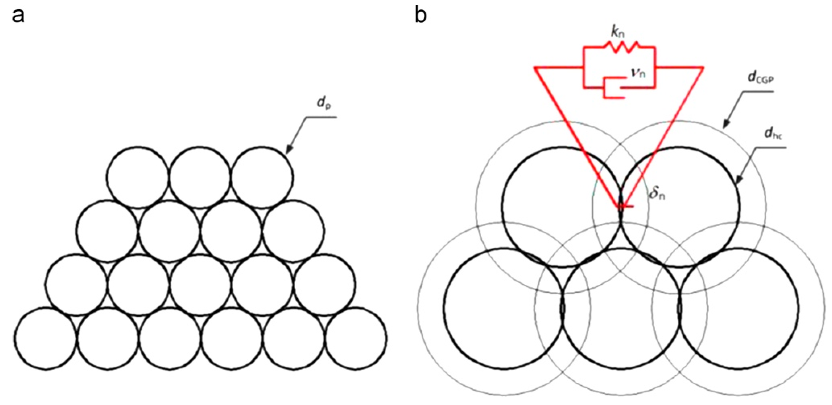
3.2.1. Compact Grains

In the majority of the coarse graining approaches, the assumptions on the conservation of mass, volume and density of the particles apply in a similar fashion. Grains are assumed to be compact (i.e., non-porous) and account for a given number of particles. The total mass of the solid for particles and grains is set to be the same. The total volume is also typically set to be constant. All grains represent the same number of particles and, for monodisperse systems, are monodisperse. Therefore, the following relations apply:

$$M_{TOT}={\sum }_{n_g}{m}_g={\sum }_{n_p}{m}_p;$$

(22)

$$V_{TOT}={\sum }_{n_g}{V}_g={\sum }_{n_p}{V}_p;$$

(23)

$${\rho }_g={\rho }_p;$$

(24)

$$m_g=n_{CG}{m}_p.$$

(25)

From the relation between the grain and particle size ($d_g=f{d}_p$, see Table 1), it follows that

$$n_{CG}=f^3.$$

(26)

Bearing in mind that the grains are assumed spherical, the constraint of same volume is equivalent to saying that the solids’ and gas volume fractions in a given region of the fluidized bed will be automatically maintained, i.e.,

$${\epsilon }_g={\epsilon }_p,$$

(27)

as the packing degree of spheres is known to be independent of size.

3.2.2. Porous Grains

For fast moving systems, such as risers and turbulent or fast-fluidized systems, the interplay between contact and hydrodynamic forces is shifted towards the latter, or at least dense regions are more limited in space. In addition, the scale of the systems is generally big, so coarse grids for the fluid are also necessary to keep the simulation feasible. For these complex multiphase and highly multiscale dynamical systems, coarse graining of DEM may require special treatments. A specific strategy was introduced by Lu et al. [16], in the context of the Energy-Minimization Multi-Scale (EMMS) method for the simulation of circulating fluidized bed reactors. Coarse grains represent both a given number of actual particles and the void among them and are introduced to represent an intermediate scale between that of the particles, on one side, and that of the typical heterogeneous structures (e.g., clusters), on the other side (Figure 3).

The grain voidage is assumed to be the same as the voidage surrounding it. So, for 3D systems,

$$n_{CG}=f^3\left(1-{\epsilon }_{CGP}\right),$$

(28)

where ${\epsilon }_{CGP}$ is the void fraction of the grain. Isolated grains are effectively representative if the convective transport mechanism of its elementary particles dominates over the diffusional counterpart.

The scaling correlation for mass is:

$$m_g=m_p f^3 \left(1-{\epsilon }_{CGP} \right).$$

(29)

3.3. Contact Interaction: Linear Spring-Dashpot-Slider Model

3.3.1. Constant Absolute Overlap Models

One of the most detailed treatment and extensive application of the coarse graining procedure with the linear contact model was given by Sakai and coworkers, who introduced it to model a pneumatic conveying line [23] and later applied it for several fluidized bed cases [61,62,63,64,65,66]. They based their derivation on imposing the conservation of the typical energy contents of the particle/grain system before and after the collisions.

The grains are assumed to move with the same velocity as the average velocity of the actual particles they represent (Figure 4). More simplistically, grains represent actual particles that move all with the same velocity, which is also equal to the grain velocity, i.e.,

$$v_g=v_p.$$

(30)

All particles are assumed to rotate also with the same angular velocity, which is not the same as the grain’s, as shown below.

The total translational and rotational kinetic energy of a grain can be expressed in terms of the sum of the corresponding energies of the represented particles:

$$\frac{1}{2}{m}_g{v}_g^2+\frac{1}{2}{I}_g{\mathsf{\omega }}_g^2={\sum }_{n_{CG}}\left(\frac{1}{2}{m}_p{v}_p^2+\frac{1}{2}{I}_p{\mathsf{\omega }}_p^2\right)=f^3\left(\frac{1}{2}{m}_p{v}_p^2+\frac{1}{2}{I}_p{\mathsf{\omega }}_p^2\right).$$

(31)

The equivalence of the rotational kinetic energy requires that the grain rotational velocity is smaller than the value of the actual particles:

$${\mathsf{\omega }}_g=\frac{{\mathsf{\omega }}_p}{f},$$

(32)

as it can be easily verified by considering that $I_g=\frac{2}{5}{m}_g{R}_g^2=\frac{2}{5}{f}^3{m}_p{f}^2{R}_p^2=f^5{I}_p$ and equating the rotational kinetic energies appearing in Equation (31). Owing to the derivative and integration of the angular velocity, it follows that the same relation applies also to the rotation, $\theta$, and angular acceleration, $\alpha$:

$${\theta }_g=\frac{{\theta }_p}{f},$$

(33)

$${\alpha }_g=\frac{{\alpha }_p}{f}.$$

(34)

The fact that collisions of grains occur in well-defined instants requires the assumption that all represented particles would collide in that same moment. Consequently, the impact of two grains leads to the consideration of the impact of all the represented particles. Following the results of Equation (31), Sakai et al. [23] set the visco-elastic/frictional interaction forces to manifest the same dependence as the energies, yielding a contact force $f^3$ times greater than that between the actual particles.

Thus, the normal component is:

$$F_{cn,g}^{}=f^3{F}_{cn,p}^{}=f^3\left(-K_n{\overline{\delta }}_{n,p}-{\eta }_n{\overline{v}}_{n,p}\right).$$

(35)

The particle relative overlap and velocity are replaced by the same quantities for the grain, giving:

$$F_{cn,g}^{}=f^3\left(-K_n{\delta }_{n,g}-{\eta }_n{v}_{n,g}\right).$$

(36)

Before discussing the tangential force, let us present the considerations on the integration time-step, set to be for the grains the same as the value for the particles:

$$\Delta t<2\pi \sqrt{\frac{m_g}{K_{ng}}}=2\pi \sqrt{\frac{f^3{m}_p}{f^3{K}_{np}}}=2\pi \sqrt{\frac{m_p}{K_p}}.$$

(37)

It is clear from the analogy between the grain stiffness, $K_{ng}$, and the particle stiffness, $K_{np}$, that the normal force-displacement dependence in Equation (36) is interpreted as a scaling law for the stiffness and damping coefficient of the grains, as follows:

$$K_{ng}=f^3{K}_{np} \mathrm{and} {\eta }_{ng}=f^3{\eta }_{np}.$$

(38)

The interesting consequence of such parameter scaling is that the coefficient of restitution of the grains is equal to that of the particles, as it can be easily derived from Equation (9). Therefore, also the dissipated energy during collisions is kept constant.

For the tangential component, in the case of adhering contact surfaces:

$$F_{ct,g}^{}=f^3{F}_{ct,p}^{}=f^3\left(-K_t{\overline{\delta }}_{t,p}-{\eta }_t{\overline{v}}_{t,p}\right),$$

(39)

in which the displacement and velocity are to be calculated at the point of contact between the surfaces. Considering that the grain rotation and angular velocity scale inversely and the radius scales directly with $f$, the displacement and velocity at the contact point of the grain are maintained similar to the ones of the particles. Following the same approach as for the normal force:

$$F_{ct,g}^{}=f^3\left(-K_t{\delta }_{t,g}-{\eta }_t{v}_{t,g}\right).$$

(40)

This can be effectively interpreted as a scaling law for the tangential stiffness and damping coefficient of the grains, as follows:

$$K_{tg}=f^3{K}_{tp},$$

(41)

$${\eta }_{tg}=f^3{\eta }_{tp}.$$

(42)

One of the consequences of such choice is that the tangential to normal stiffness ratio remains constant.

Finally, for sliding contact surfaces, Coulomb’s limit is scaled simply according to:

$$F_{ct,g}^{}\le \mu f^3|F_{cn,p}^{}\left|=\mu |F_{cn,g}^{}\right|,$$

(43)

which corresponds to maintaining the same coefficient of friction between the grain and the particles, i.e.,

$${\mu }_g={\mu }_p.$$

(44)

Recently Cai and Zhao [67] noted that for the conservation of the dissipation during sliding the friction coefficient should be scaled according to

$${\mu }_g=\frac{{\mu }_p}{\sqrt{f}}.$$

(45)

It is interesting to note that the $f^3$ scaling of the stiffness leads to the same maximum overlap between colliding grains as for colliding particles, for impacts at the same velocity. Indeed, the oscillation frequency of a linear mass-spring system depends on the ratio between the spring constant and the mass (both scaled with $f^3$), and the maximum overlap is given by the impact velocity divided by this frequency. The elastic energy upon compression is also among the conserved quantities for grains with respect to the particles [62]:

$$E_g^{el}=\frac{1}{2}{K}_{ng}{\delta }_{n,max}^2=\frac{1}{2}{f}^3{K}_{np}{\delta }_{n,max}^2=n_{CG}{E}_p^{el}.$$

(46)

A similar approach was adopted by Benyahia and Galvin [68], who assumed a smaller number of special particles (the grains) to be representative of all actual particles. Each grain has a statistical weight, which is equivalent to $n_{CG}$ in the present notation. An illustrative scheme was reported in a later publication (Figure 5). In their analysis on the concept of parcels in the MP-PIC approach (see [22,69]) simulated like DEM grains under shear and riser flow conditions, the authors also found a sensitive dependence on the scaling of the stiffness and damping coefficient, proposing a proportionality with the mass (i.e., $f^3$ factor) for their scaling. Similarly, a fixed tangential to normal stiffness ratio is used.

Motivated by the differences in the velocity distribution and granular temperature, they addressed the reduced amount of dissipation by introducing a modification to the restitution coefficient of the grains compared to the value for the actual particles. The assumption was that during a grain-grain collision, each particle represented by one grain was thought to collide with all the particles in the other grain. and later further discussed in Lu et al. [70].

The proposed coefficient of restitution for the grains is related to that of the particles by

$$\frac{\ln \left(e_g \right)}{\ln \left(e_p \right)}=\sqrt{n_{CG}}\frac{\sqrt{1-\frac{{\ln }^2\left(e_p\right)}{{\ln }^2\left(e_p\right)+{\pi }^2}} }{\sqrt{1-\frac{n_{CG}{\ln }^2\left(e_p\right)}{{\ln }^2\left(e_p\right)+{\pi }^2}}}.$$

(47)

The denominator is defined up to a maximum coarse graining degree $n_{CG}$ for each $e_p$. For the frequent case in which $\frac{n_{CG}{\eta }_n^2}{2K_n{m}_p}\ll 1$, the grain restitution coefficient can be conveniently calculated by

$$e_g=e_p^{\sqrt{n_{CG}}},$$

(48)

which incidentally removes the limitation on the maximum $n_{CG}$ and exhibits an intuitive tendency $e_g\to 0$ as $n_{CG}\to \infty ,$ for any value of the original coefficient of restitution $e_p$. Benyahia and Galvin reported a significant improvement of the results for both the shear flow and riser flow in maintaining consistency upon scaling with $n_{CG}$ [69]. The following different scaling of the restitution coefficient, based on the kinetic theory of granular flows, was used in a later work [71],

$$e_g=\sqrt{1+\left(e_p^2-1\right)f}.$$

(49)

Equation (49) produces a slightly slower decrease of $e_g$ than Equation (48) at low coarse graining factors $f$. However, it also sets a maximum degree of coarse graining $f<\frac{1}{1-e_p^2}$ to yield a real value of $e_g$.

Hilton and Cleary [26,27] adopted a similar approach and coarse graining scaling laws, additionally estimating the computational load to scale with order $O\left(f^{-3}\right)$.

3.3.2. Constant Relative Overlap Models

Starting from a slightly different point, Radl et al. [25] also examined the coarse graining of particles in parcels treated DEM-like for granular jet applications. Their approach differs from the one presented above for two important aspects: the conserved properties and a distinction between the dense and dilute regions, the latter of which requiring a velocity relaxation. The point of departure is the non-dimensional form of the equations of motion of a particle (or grain), for which all quantities are to be conserved when moving from particles to grains.

The main difference concerns the contact parameters, which are shown to scale according to:

$$\frac{K_{ng}}{R_g}=\frac{K_{np}}{R_p};$$

(50)

$$\frac{{\eta }_{ng}}{R_g^2}=\frac{{\eta }_{np}}{R_p^2}.$$

(51)

Such dependence can be explained by the fact that the maximum absolute overlap of the grains is also scaled compared to the original particles. In particular, the relative maximum overlap is kept constant, for example in terms of similar percentage of the radius, i.e.,

$$\frac{{\delta }_{ng,max}}{R_g}=\frac{{\delta }_{np,max}}{R_p}.$$

(52)

It shall be noted that the elastic energy stored during collisions is preserved also with this scaling. A smaller stiffness compared to the previous scaling affects other dynamic properties of the collision, such as the duration. It turns out that the collision time scales linearly with the coarse graining degree:

$${\tau }_g=2\pi \sqrt{\frac{m_g}{K_{ng}}}=f2\pi \sqrt{\frac{m_p}{K_{np}}}=f{\tau }_p.$$

(53)

However, the duration of collisions is generally smaller by orders of magnitude than any other characteristic time, at least for fluidized bed applications. On the other hand, the integration time step can be increased, with further additional computational savings. This same coarse graining approach was used by Nasato et al. [72].

Similar to Benhyaia and Galvin [68], Radl et al. [25] recognized the need for additional dissipation to take into account intra-grain collisions between the particles, particularly in dilute regions. For this term, the authors derived a modified version of the velocity relaxation model of O’Rourke and Snider [73]. Since the formulation requires the definition of several parameters, a complete discussion is omitted, and the original source is recommended to the interested reader.

3.3.3. Contact between Porous Grains

For porous grains to be used in EMMS-DPM [16], contact model during collisions is to be adapted. The soft grains are thought to be able to compress until the elementary particles reach close packing, i.e., ${\epsilon }_{mf}$. The grain has an external diameter $d_g$ and an internal “hard-core” diameter, defined by

$$d_{hc}={\left(1-{\epsilon }_{CGP}\right)}_{}^{\frac{1}{3}}{d}_g,$$

(54)

in which the voidage is

$${\epsilon }_{CGP}=\max \left({\epsilon }_{mf},{\epsilon }_{CGP,min}\right),$$

(55)

where ${\epsilon }_{CGP,min}$ depends on EMMS properties such as the minimum cluster diameter and the maximum cluster voidage.

The linear spring-dashpot model is used to model contact between grains in the normal direction, which is detected whenever the hard cores of the grains come into contact (Figure 6). Inter-grain collisions are treated using a slightly simplified version of the linear spring-dashpot model. The normal spring stiffness is set at the minimum value that ensures stability. Normal damping is applied through the coefficient of restitution, which is determined based on the same dissipation of total energy as the real particles and intra-grain collisions, i.e.,

$$e_g=\sqrt{1+\left(e_p^2-1\right)f{\left(1-{\epsilon }_{CGP}\right)}^{\frac{1}{3}}} .$$

(56)

The tangential contact is modelled using a purely dissipative force capped to Coulomb’s limit for sliding, with a ratio of tangential to normal damping coefficient fixed at $\sqrt{0.8}$. The time step is set as a fraction of the collision duration of based on the mass of the grain, i.e., $\mathsf{\Delta }t=2\pi \sqrt{\frac{m_g}{K_{ng}}}$, benefitting from the computational advantage of this choice. More details are available in the original manuscript.

3.3.4. Summary of Coarse Graining Approaches for the Linear Model

A summary of the coarse graining scaling factors for the linear spring-dashpot-slider model is reported in

Table 2. Summary of the scaling factors for the linear spring-dashpot-slider model.

Equal Dissipation Approaches, i.e., $e_g=e_p$
	Stiffness (N) ${\mathit{K}}_{\mathit{n}\mathit{g}}/{\mathit{K}}_{\mathit{n}\mathit{p}}$	Damping (N) ${\mathit{\eta }}_{\mathit{n}\mathit{g}}/{\mathit{\eta }}_{\mathit{n}\mathit{p}}$	Stiffness (T) ${\mathit{K}}_{\mathit{t}\mathit{g}}/{\mathit{K}}_{\mathit{t}\mathit{p}}$	Damping (T) ${\mathit{\eta }}_{\mathit{t}\mathit{g}}/{\mathit{\eta }}_{\mathit{t}\mathit{p}}$	Friction ${\mathit{\mu }}_{\mathit{g}}/{\mathit{\mu }}_{\mathit{p}}$
Constant absolute overlap models (see, among others, [23,26,68])	$f^3$	$f^3$	$f^3$	$f^3$	$1$
Constant relative overlap models (see, among others, [25,72])	$f$	$f^2$	$f$	$f^2$	$1$
Additional (intra-grain) dissipation approaches, i.e., $e_g<e_p$
	altered dissipation			notes
Simplified dissipation scaling (Benyahia and Galvin (2010) [68])	$e_g=e_p^{\sqrt{n_{CG}}}$			valid if $\frac{n_{CG}{\eta }_n^2}{2K_n{m}_p}\ll 1$, otherwise see Equation (47)
KTGF based scaling (Lu et al. (2018) [71])	$e_g=\sqrt{1+\left(e_p^2-1\right)f}$			from the KTGF; limited by $f<\frac{1}{1-e_p^2}$
EMMS-DPM (Lu et al. (2014) [16])	$e_g=\sqrt{1+\left(e_p^2-1\right)f{\left(1-{\epsilon }_{CGP}\right)}^{\frac{1}{3}}}$			from CG in EMMS; valid for grains with “porosity”

(N): normal; (T): tangential.

. Note that scaling imposing the same coefficient of restitution (i.e., $e_g=e_p$) is equivalent to using the scaled damping coefficient.

3.4. Contact Interaction: Hertz-Based Modelling

Non-linear Hertz-based models are common in DEM simulations of quasi-static systems, when interactions at particle–particle and particle–wall contacts are crucial to represent bulk stress–strain relationships. Nonetheless, contacts and dissipation in fluidized beds can become important, for example when cohesive interactions are also involved. As it will be shown, scaling of Hertz-based model is not particularly complicated.

An accurate treatment of coarse graining for Hertz-based contacts was reported by Bierwisch et al. [24] in the framework of a simulation and experimental study of a cavity filling process. It is based on the same postulates regarding the conservation of the density of various energy contributions. A similar gravitational energy density requires the granular phase to have the same total solids mass and volume and each grain has the same density of the particles; this condition also leads to a similar volume fractions for spherical particles.

Imposing the same kinetic energy density requires all the representative particles to move with the same velocity as the grains. The condition to maintain the dissipated energy during collisions constant requires the collision of one grain to dissipate as much as $n_{CG}$ collisions of the represented particles, i.e.,

$$E_{dg}=\frac{1}{2}{m}_g\left(v_{0g}^2-v_{fg}^2\right)=\frac{1}{2}{n}_{CG}{m}_p\left(v_{0g}^2-v_{fg}^2\right).$$

(57)

If the initial collision velocity is the same, i.e., $v_{0g}=v_{0p}$, and the coefficient of restitution is correspondingly the same, i.e., $e_g=e_p$, so that the final velocity is also equal, then the last term of Equation (57) is equal to $n_{CG}{E}_{dp}$.

The coarse grain model for the contact forces is obtained by examining the equations of motion for the contacting particle. In the present notation, for the normal and tangential direction and neglecting the cohesive forces, they read

$$m_{eq}{a}_n^{}=-\frac{2}{3}{E}_{eq}\sqrt{R_{eq}{\delta }_n}{\delta }_n-{{\eta }^{\prime }}_n\sqrt{R_{eq}{\delta }_n} v_n$$

(58)

and

$$m_{eq}{a}_t^{}=-\min \left[\mu \left|\frac{2}{3}{E}_{eq}\sqrt{R_{eq}{\delta }_n}{\delta }_n-{{\eta }^{\prime }}_n\sqrt{R_{eq}{\delta }_n} v_n\right|, K_t\sqrt{\frac{{\delta }_n}{R_{eq}}}\left|{\delta }_t\right|\right]sgn\left({\delta }_t\right).$$

(59)

Note that the rotational motion was not considered [24]. By dimensional analysis of the equations and the study of relative dimensionless group, conservation of the energy densities leads to the following dependencies:

$$E_{eq,g}=E_{eq,p}; \frac{{{\eta }^{\prime }}_{ng}}{R_{eq,g}}=\frac{{{\eta }^{\prime }}_{np}}{R_{eq,p}}; \frac{K_{tg}}{R_{eq,g}}=\frac{K_{tp}}{R_{eq,p}}.$$

(60)

A comparison with the linear model reveals that the non-linear model naturally leads to a constant relative overlap for collisions at the same velocity. It can be observed that maintaining the same physical parameters, i.e., $\rho$, $E$, $\nu$, leads to a consistent coarse graining approach.

It should be noted that the formulation of the velocity dependent dissipative force shows some differences with respect to Equation (15). A corresponding dependence of ${\eta }_n^H$ implies a quadratic scaling with the coarse graining factor (see e.g., [44]), i.e., ${\eta }_n^H\propto f^2$, in order to yield the same constant coefficient of restitution, i.e., $e_g=e_p$, similar to previously illustrated linear models.

Overall, the force contributions are shown to scale by a factor of $f^2$, a fact that allows also solid stress distribution in dense regions to remain unchanged [24]. Indeed, this was also confirmed in the analysis of scaling in simulated experiments of uniaxial compression tests (stress–strain relationship) by Thakur et al. [74]. They reported correct scaling of the results with a linear up-scaling of the normal stiffness with the coarse graining degree, which is the case here, as proved by the constant $E_{eq}$ and the linear dependence on $f$ of both $R_{eq}$ and ${\delta }_n$ in Equation (10).

In a similar way, Nasato et al. [72] examined the Hertz-based normal contact dependence on particle size and found that it is scale independent. This means that parameters such as Young’s modulus and Poisson ratio are set equal.

The consequence of the relative overlap kept constant, i.e.,

$$\frac{{\delta }_{ng,max}}{R_g}=\frac{{\delta }_{np,max}}{R_p},$$

(61)

is that the collision duration and integration time-step increase linearly with the coarse graining degree:

$${\tau }_g=f{\tau }_p\to \mathsf{\Delta }{t}_g=f\mathsf{\Delta }{t}_p.$$

(62)

The same model was used in CFD-DEM simulation of dense medium cyclones by Chu et al. [75].

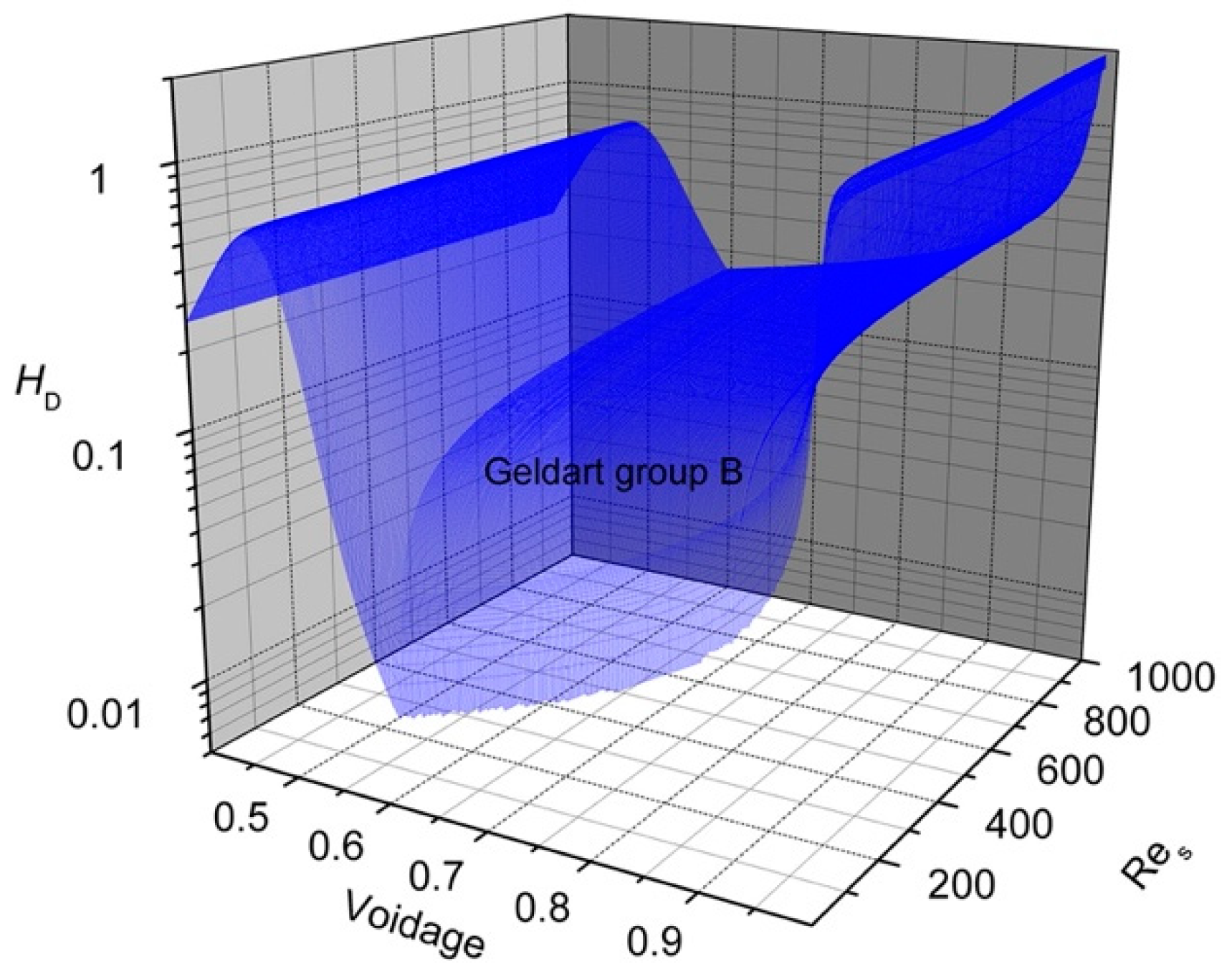
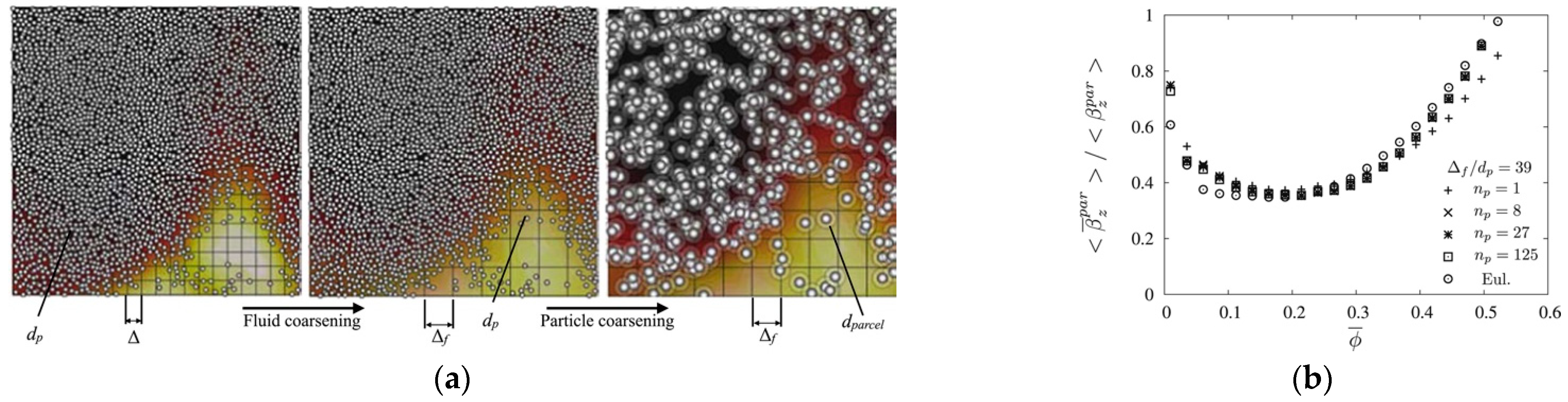
3.5. Hydrodynamic (Drag and Pressure Gradient) Forces

For the drag force, a large consensus points to the need that grains experience the same total force as all the represented particles under the same conditions. For compact coarse grains, this corresponds to assuming the following simple relationship

$$F_{dg}=n_{CG}{F}_{dp}=f^3{V}_p\frac{{\beta }_p}{1-\epsilon }\left(u-v_p\right)=V_g\frac{{\beta }_p}{1-\epsilon }\left(u-v_g\right),$$

(63)

in which ${\beta }_p$ is to be calculated using the particle properties, not the grain properties, and the fact that $v_p=v_g$ was used. An implicit assumption of Equation (63) is that all represented particles are close enough to one another to experience the same relative velocity and voidage.

A similar scaling applies to the pressure gradient force:

$$F_{bg}=n_{CG}{F}_{bp}=f^3{V}_p\nabla p=V_g\nabla p.$$

(64)

For the case of non-compact, porous grains, the following modifications were proposed in the context of the EMMS-DPM model:

$$F_{dg}=\frac{V_g{\beta }_{ph}}{1-\epsilon }\left(1-{\epsilon }_{CGM}\right)\left(u-v_g\right)$$

(65)

and

$$F_{bg}=V_p\left(1-{\epsilon }_{grain}\right)\nabla P.$$

(66)

In Equation (65) the parameter ${\beta }_{ph}$ is the conventional coefficient in the drag expression multiplied by a correction factor known as heterogeneity index, ${\beta }_{ph}={\beta }_p{H}_D$, defined by

$$H_D=a{\left(R{e}_p+b\right)}^c,$$

(67)

in which $R{e}_p$ is the particle Reynolds’ number and the constants $a$, $b$ and $c$ are complex functions of the local voidage $\epsilon$. A representative plot of the heterogeneity index for a particle of Geldart’s group B is shown in Figure 7.

At this point it is worth noting that the use of larger particles (the grains) pushes towards the use of a coarser Eulerian grid for the fluid. In turn, if the cell to grain size ratio is kept constant, increasing the coarse graining degree quickly brings about the issues associated with the use of a large cell size compared to the particle size [77]. Therefore, either the need for grid size scaling or sub-grid corrections was recognized and pointed out [78,79,80], as a common requirement also for Eulerian-Eulerian and MP-PIC simulations on coarse grids (Figure 8a). For example, Radl and Sundaresan [78] examined the vertical upflow in periodic domains at different Reynolds’ number and solids concentration, later focusing specifically on fluid and particle coarsening for parcel-based simulations [81]. Figure 8a shows graphically a typical effect of the use of coarse-grained parcels, which requires fluid grid coarsening. Figure 8b shows the effect of the fluid grid coarsening (filter-to-particle size ratio = 39) on the normalized drag coefficient as a function of porosity and the number of particles per parcel. Remarkably, the dependence on voidage of the correction on the drag coefficient (Figure 8b) appears in reasonable agreement with the same dependence of the heterogeneity index in the EMMS model (Figure 7), at least for sufficiently high Reynolds’ numbers, although they arise from apparently different points of departure. Both plots highlight the strong need for corrections to the conventional drag models for flow in risers and if significant particle coarse graining is targeted.

3.6. Cohesive Force Modelling

The scaling of cohesive forces is less well established than contact and hydrodynamic forces, so the models appearing will be listed as presented by the authors. On the other hand, scaling for cohesive solids has more severe implications on the accuracy of the computations [82].

In their analysis of the coarse graining using Hertz contacts, Bierwisch et al. [24] presented also the scaling rule for the Johnson, Kendall, Roberts (JKR) theory of cohesion, considered without hysteresis. The material parameter is the work of adhesion per unit contact area $w$, which is clearly proved to depend on the coarse graining degree

$$\frac{w_g}{R_{eq,g}}=\frac{w_p}{R_{eq,p}},$$

(68)

leading to a cohesive force scaling with $f^2$.

A different scaling for the JKR cohesive model was recently introduced by Chen and Elliott [83], who found correct scaling of the cohesive force and surface energy with $f^3$ and $f^2$, respectively. However, the work of adhesion was also scaled to keep the same dissipative restitution (i.e., rebound vs. impact velocity) according to $f^3$, which led to the corresponding scaling of the Young’s modulus $E_g=f^{2.5}{E}_p$ and the overlap during collisions is obtained to be the same, i.e., ${\delta }_{ng}={\delta }_{np}$.

In Sakai et al. (2012) [63], the coarse grain scaling on DEM is presented including van der Waals interactions. Similar to the other phenomena, the interparticle cohesion on one grain is applied assuming that all represented particles interact simultaneously with all the particles represented by the close grain. Scaling of the force is initially set to depend on $f^3$, in analogy with the other force contributions. Considering that the inter-particle distance, $h_p$, may be smaller than the inter-grain distance, $h_g$, the following correction is proposed

$$h_g=\frac{h_p}{f}.$$

(69)

Thus, the overall cohesive force scales with $f^2$

$$F_{kg}=f^3\frac{H_A{d}_g}{6h_g^2}=f^2\frac{H_A{d}_p}{6h_p^2}.$$

(70)

where the Hamaker constant is assumed to be the same for grains as for the particles. The cohesive force does not change the contact force, and the DEM time step is set to be the same as the cohesionless case.

In Mokhtar (2012) [59], the Similar Particle Assembly model [20] is integrated with the cohesive liquid bridge force, which is not scaled. Grains have diameter $f$ times that of the particle, with equal density and assuming same velocities. The contact model is LSD. The forces are scaled with the third power of $f^3$, but all other properties are kept equal to the original particle case, including the DEM time step.

More recently, Chan and Washino [84] proposed a coarse graining strategy for liquid bridge cohesive interactions between grains for applications in agitated mixers. They based the derivation on the assumption that interfacial interactions such as the liquid bridge cohesion shall scale with $f^2$. Therefore, in analogy with the $f^2$ dependence of the (Hertz-based) contact force, also the liquid bridge force (capillary plus normal and tangential viscous contributions) is calculated by

$$F_{kg}=f^2{F}_{kp}.$$

(71)

The following additional parameter scaling were shown to be successful.

Liquid bridge volume:

$$V_{lg}=f^3{V}_{lp};$$

(72)

Separation distance:

$$S_g=S_p;$$

(73)

Rupture distance:

$$S_g^{\prime }=S_p^{\prime }.$$

(74)

The most recent investigation by Tausendschön et al. [85] concerns a detailed analysis of liquid bridge and van der Waals cohesive force scaling in coarse grained CFD-DEM simulations of periodic fluidized systems. In the context of contact scaling based on maintaining constant the relative overlap (see Table 2), starting from three different theoretical bases led essentially to confirm correct scaling if the surface tension and liquid viscosity scale linearly with $f$ and the Hamaker constant scales with $f^3$. In addition, they pointed their attention to the significant role that the field smoothing filter plays in hydrodynamics for grain sizes growing similar to or larger than cell sizes.

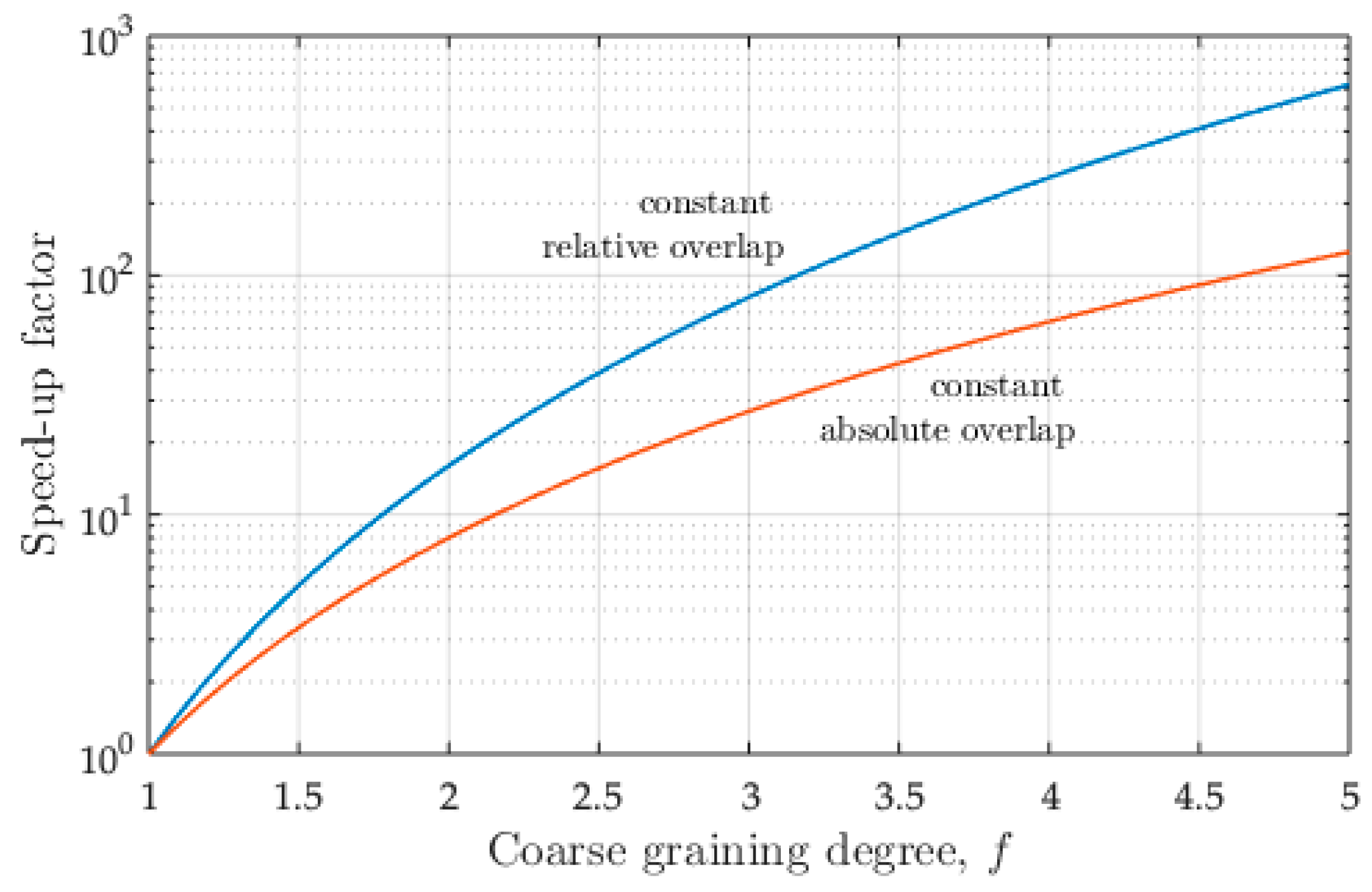
4. Computational Savings

As anticipated in the introduction, the main advantages of the coarse graining approach and its most attractive features are the conceptual simplicity, which translates into simple steps to deploy it into a code, and the computational saving compared to classical DEM. For nearly all the approaches presented so far, the changes to the code required to implement coarse graining are very limited. The core of the coarse graining lays in adapting the parameters so that the (same) DEM equations of motion and CFD part provide the results in terms of grains instead of the particles. Therefore, another attractive property of the method is the ease of implementation.

The theoretical scaling of the computational time required to simulate a given time can be estimated assuming an inverse proportionality of the total time on the integration time step (realistic) and on the number of particles (pessimistic). As discussed in Section 3, the key step determining the time step is the contact model: with the constant absolute overlap linear model, the time step with grains is the same as the one with particles; with the constant relative overlap linear model and the Hertz model, the time step increases proportionally with $f$. The number of particles scales with $f^3$. The coarse graining factor represent the ratio between the grain size and the particle size. Therefore, constant absolute overlap and constant relative overlap schemes scale with the 3rd and 4th power of the coarse graining factor, respectively. A plot of these theoretical speed-up trends is shown in Figure 9. In the best case (constant relative overlap), grains twice as big as the particles they represent ($n_{CG}=8$) already allow an estimated speed-up = 16. With grains just three times bigger ($n_{CG}=27$), the speed-up is greater than 80. Eighty times faster!

It is worth mentioning that the above estimate is not optimistic, as a decrease in the number of particles is very likely to produce a higher than linear decrease in CPU time. However, in CFD-DEM simulations part of the time is also spent in the CFD part, with overall savings that can be less striking.

To show examples of performance achievable with coarse graining CFD-DEM, selected applications from the literature are listed in

Table 3. List of selected applications of coarse graining approaches and corresponding performance improvements.

Reference	Investigated CG Range	Typical Performance
[19]	$f=1, 3, 6$	speed-up = 15 ($f=3$), 50 ($f=6$)
[60]	$f=1 \mathrm{to} 13.3$	$\log CPUtime=-2.55·\log f$
[20]	$f=200$	8 k grains for 64 billion particles
[24]	$f=4.7, 9.4, 18.8$	at $f=9.4$, 66 k grains for 60 M particles
[68]	Shear flow: $n_{CG}$ = 1,2,5,10   ($f=1, 1.25, 1.71, 2.15)$ Periodic riser: $n_{CG}$ = 10, 20, 50, 100 (relative $f^{*}=1, 1.25, 1.71, 2.15$)	speed-up: 1, 3.6, 26, 102 relative speed-up *: 1, 3.3, 11, 15
[61]	$f=1, 2, 3$	speed-up: 1, 3, 4.3,
[26]	$f=1.5, 2, 3$	speed-up: 4.2, 15.7, 68.6
[16]	$\mathrm{CFB}1: f=1, 2, 3, 4$ $\mathrm{CFB}2: f=1, 6, 8, 10$ $\mathrm{CFB}3: f=10$	48 k grains for 1.6 M particles 190 k grains for 4.1 M particles 14 M grains for a real CFB loop
[86]	$f=2, 3$	speed-up = 8.2, 29
[87]	$f=5, 10$	at f = 5, speed-up = 625 (estimated); for the relative f* = 2, speed-up = 6.
	$f=5, 10, 15$	speed-up * = 1, 35, 131
[80]	$f=0.8, 2$	speed-up $\propto f^3$
[85]	$f=2, 4$	speed-up = 14, 30

^* Relative coarse graining degree and speed-up with respect to the lowest $f$.

.

Considering the one decade since introduction and widespread diffusion, it must be admitted that the question on to what extent the highly attractive savings come at the cost of accuracy is still not fully answered. To investigate validation at extreme coarse graining, a recent application in fluidized beds involved grains with $n_{CG}=\mathrm{300,000},$ i.e., $f\approx 67$ [33], but the expected speed-up was not reported.

5. Applications to Bubbling/Spouted Beds

5.1. Bubbling/Spouted/Liquid Fluidized Beds

Initial verification and validation studies have been carried out on small pseudo-2D geometries and bubbling fluidization conditions [61,62,63]. More recently, CG-DEM was simulated in lab-scale bubbling beds with immersed tubes [66]. Simulations have been reported on the small-scale NETL bubbling bed challenge [88], including also the benefit of hard-sphere model for the collisions, which further considerably improves numerical efficiency.

Coal gasification was studied in a bubbling fluidized bed including heat transfer and heterogeneous chemical reactions, which allowed the influence of the operating parameters to be effectively characterized [89]. Using a commercial software, the steam gasification of biomass was studied in a bubbling bed including heat transfer, chemical reaction and particle shrinkage [34,90]. The fast pyrolysis of biomass was investigated using a multiscale approach, combining coarse-grain particle scale simulations with reactor scale modelling [91,92]; similarly, coarse grain DEM-CFD combined with reduced-order modelling was used to simulate a pilot-scale updraft coal gasification reactor [93]. Bubbling fluidization of a sand-biomass mixture was compared against experiment for degree of mixing and pressure drop (average and fluctuations) [94,95]. Different testing methods for measuring solids distribution have been compared and improved by simulating the so-called “travelling fluidized bed” [96]. A coarse-graining application to segregation in vibrated fluidized beds can be found in Reference [97].

Very long simulations have been achieved using EMMS-DPM for the methanol-to-olefin process [98] (Figure 10), reaching as long as 8 h of simulated time. Similar long runs were obtained with a similar model for the simulation of a continuous compartment fluidized bed, with computation of the residence time distribution of the polydisperse fluidized solids [99].

Solids motion in spouted beds was investigated with focus on the solids and velocity distributions, pressure drop and solids mixing [86]. The effect of gas inlet in prismatic spouted beds was also investigated successfully [100]. As a peculiar application, intermittent fluidization during solids discharge of lunar regolith simulants was shown to be successfully simulated [101].

Simulations of a liquid-fluidized reactor, including chemical conversion were reported in [70].

5.2. Circulating Fluidized Beds and Cyclones

Since the introduction of the coarse grain technique, applications in riser flow and CFBs have started to appear in noticeable number. Several periodic systems were investigated, mostly with the objective to improve understanding, characterize the influence of the coarse graining degree and grid size. Examples of such analyses are [68,78,80,81].

Larger scale riser flow simulations were carried out for energy applications, such as for a chemical looping system [102] and for a fluidized bed carbonator [103,104], in both cases using a commercial software. A complex combination of tools including coarse grain CFD-DEM was successfully utilized to simulate the multiphase flow of liquid, magnetite fine particles, coal particles, with the formation of an internal air core [105]. The combined use of EMMS-DPM has also been extensively used for riser flow, e.g., [16,106].

6. Recent Promising Extensions and Open Problems

6.1. Physical Models

Since its introduction, the concepts of parcels and grains appeared to be limited to a constant (in time) and uniform (across the system) number of particles per grain. This restriction had severe implications from the point of view of industrial applicability, as real particles are all but monodisperse spherical particles. On the other hand, DEM is notorious for its capability to treat particle individually, so potentially each one different from the rest. In one of their recent efforts, Lu et al. [71] introduced two strategies to deal with coarse graining of a particle system with size distribution. The two strategies differ for the constant quantity of the coarse graining: in strategy SSW (same statistical weight), the grains contain the same number of particles; in the SSP (same size parcel), all the grains share the same size (Figure 11). As a consequence, in the former case, there is a size distribution of the simulated grains; in the latter, there is a number distribution of represented particles by each grain and all grains are monodisperse. The technique was successfully applied to the fluidization of Geldart’s group A (FCC) and group B (glass beads) particles and showed that the agreement with pure DEM and experiments is reasonable. Lu et al. [71] conclude that the accuracy of the SSW method at low velocity is higher than that of the SSP method. At higher velocity their accuracy is similar. On the other hand, the monodisperse nature of the grains with the SSP strategy allows for improvements in the computational efficiency, avoiding the limitation on the time step imposed by smaller particles/grains.

Another improvement in coarse-grain simulations concerns accurate procedures for scaling heat transfer parameters. This has been thoroughly investigated by Lu et al. [107], who determined scaling parameters for both the particle-fluid-wall transfer mechanism and the direct contact heat transfer mechanism. The results indicate that: the particle minimum distance and gas layer length must be kept constant in dimensionless terms, i.e., they should scale with the coarse graining degree $f$; the dimensionless particle-wall distance scales with $f^{-1}$; so, overall, the particle-fluid-wall transfer mechanism calculated using the grain properties must be scaled by

$$Q_{pfw}=\frac{Q_{pfw,g}}{f^2}.$$

(75)

Similarly, for the direct contact mechanism,

$$Q_c=\frac{Q_{c,g}}{f^{\frac{9}{4}}}\sqrt{\frac{f\left(e_p\right)}{f\left(e_g\right)}}.$$

(76)

in which $f\left(e\right)$ is an explicit function of the coefficient of restitution. Note that the result for the scaling of the direct contact mechanism assumes the linear spring-dashpot model with the same particle stiffness of the grains as the particles.

Treatment of the erosion of tubes in bubbling fluidized beds was investigated by Zhou and Zhao [108].

6.2. Computational Improvements

Recently proposed computational improvements are aimed either at extending the specific coarse graining technique beyond the previous boundaries or at combining multiple techniques to further speed up the computations, without compromising the accuracy.

Starting from the reduced particle stiffness model [109], the augmented coarse graining method for the CFD-DEM simulations of fluidized beds was proposed by Lin et al. [110], who tested the combined model in bubbling and circulating fluidized beds against experimental averaged solids velocity profiles. The computational benefits of coarse graining ($f=5$) is combined with the advantage of the reduced particle stiffness model (reduced stiffness factor = 0.01), reaching a speed-up factor of almost 5000. The actual loss in accuracy requires additional and more extensive quantification.

The multilevel coarse graining technique for DEM introduced by Queteshiner et al. [44,111] aims at making it possible to adapt the coarse graining level to different regions, so that a coarser realization is used in regions whose behavior is simpler to represent and a finer level is used in spatially confined regions of interest. Different levels are coupled by exchanging volume-average flow properties. One application is the discharge of solids from a bin, taken as reference test for comparison. It is a method with promising potential for improved accuracy and likely to be useful also in fluidized bed applications. On the other hand, the improved accuracy and representation capability comes at the cost of the computational efficiency, which deteriorates compared to pure coarse graining and further work is needed to recover as much as possible of this attractive property.

A very significant improvement in speed for computations is obtained by combining coarse graining and hard-sphere event-driven models for collisions, without compromising the accuracy of the predictions in fluidized beds, according to Lu et al. [87,88] (Figure 12). Together with coarse-graining, a corrected hard-sphere model specifically derived by the authors, formed the CGHS (coarse grain hard-sphere) model, capable of providing an overall impressive speed-up of 24 using $f=2$. The solver was fast enough to require computational times comparable with those of MP-PIC, known to be less accurate but much faster. The actual comparison with MP-PIC simulations on the same system (small-scale fluidized bed) revealed a clear superiority of the discrete CGHS model. Indeed, the conclusions of the authors are that the CGHS combinations provide an accurate and inexpensive way to simulate fluidized beds.

Finally, other dynamic coarse graining strategies were proposed by Wang et al. [112] with particle-group crushing and polymerization. The method requires additional corroboration and more extensive validation.

6.3. Open Problems

To really reach sufficient maturity and industrial relevance like it is now for CFD, the attractive computational gain achieved with coarse-grain CFD-DEM still requires substantial effort in terms of further development and validation. Not only are simulations to be confronted with full CFD-DEM results as in many of the articles cited here but also directly with experimental data, as the number of modelling “layers” and corresponding parameters is high. The coarse graining procedure enhances the importance of accurate parameters and requires closed-form procedures for particle-to-grain property scaling. Therefore, it would be highly desirable to compare simulated results with sufficiently simple experiments, whose measured data relate as directly as possible to the microscopic mechanisms that originate them.

To conclude, the following topics, insufficiently covered in previous studies, are proposed as future objectives of interest:

• Coarse graining of non-spherical particles;
• Rotational motion and rolling friction for applications e.g., in cyclones;
• Further testing on multi-component polydisperse particles, with coarse-graining of polydisperse drag;
• Hydrodynamic interactions in dilute regions (collisional regime) at extreme coarse graining degrees and with coarse grids;
• Further development of adaptive coarse graining;
• Scaling for mass transfer, chemical reactions and other cohesive interactions, e.g., triboelectric charging.

7. Conclusions

Starting from the beginning of the 2000s, a new class of methods to expand the applicability of CFD-DEM have established in the field for the simulation of fluidized beds. Thanks to their significant computational advantages, in the last decade, the coarse-graining approach has grown to become a relatively widespread technique. The present review summarizes the essential ingredients of the coarse graining method, covering in detail: contact forces (linear and Hertz-based), hydrodynamic interactions and cohesive forces for both compact and porous grains. More than one possible approach is found, depending whether the absolute or relative displacement is kept constant, and discussed. As a byproduct of this process, new links between the scaling with the linear and Hertz-based contact model are highlighted. Scaling of the most important hydrodynamic forces, drag and pressure gradient, in homogeneous systems is obtained relatively easily and ensures conservation of the pressure drop for uniform systems (e.g., the dense phase). Where heterogenous structures are dominating (e.g., clustering in risers), the use of a coarse grid for the CFD part often requires additional corrections and adjustments on the drag law. Scaling of interparticle cohesive forces depends on the force model and can be different in the case of Hamaker’s model, JKR theory or capillary interactions due to liquid bridges.

The advantages in terms of computational savings is quantified, depending on the coarse graining choice, i.e., constant absolute overlap vs. constant relative overlap models, showing 3rd or 4th power scaling, respectively. Some applications in the field of bubbling and circulating fluidized beds are illustrated, to provide a picture of the state-of-the art and showcase the explored possibilities. New extensions for accuracy improvement (e.g., handling polydisperse solids, scaling of heat transfer and adaptive coarse graining) and further computational saving (combined coarse graining hard-sphere, CGHS) are discussed.

In terms of model fundamentals, this review shows that the basic equations are ready for implementation for most applications. Thus, CGDEM simulations of fluidized bed systems can benefit from unparallel speedup factors. The loss of accuracy is generally limited, for example, if heterogeneities are not dominating, and there are no key particle-wall interactions, such as in highly complex geometries. In these cases, the actual loss is yet to be fully quantified, particularly if the coarse graining degree is high. Therefore, expected progress is in the area of validation, possibly with directly comparable experiments (see e.g., [35]) and attempts to quantify the uncertainty associated with coarse graining at different scales (see e.g., [113]). Moreover, developments to include new, locally adaptive schemes would be particularly useful. Overall, the increasing impact of the coarse grained CFD-DEM in recent years is expected to grow further and lead to widespread adoption, both in fluidized bed research and industrial applications.

References

1. Grace, J.R.; Bi, X.; Ellis, N. Essentials of Fluidization Technology; Wiley-VCH: Weinheim, Germany, 2020; ISBN 9783527340644. [Google Scholar]
2. Figaro, S.; Pereira, U.; Rada, H.; Semenzato, N.; Pouchoulin, D.; Paullier, P.; Dufresne, M.; Legallais, C. Optimizing the Fluidized Bed Bioreactor as an External Bioartificial Liver. Int. J. Artif. Organs 2017, 40, 196–203. [Google Scholar] [CrossRef] [PubMed]
3. Naghib, S.D.; Pandolfi, V.; Pereira, U.; Girimonte, R.; Curcio, E.; Di Maio, F.P.; Legallais, C.; Di Renzo, A. Expansion properties of alginate beads as cell carrier in the fluidized bed bioartificial liver. Powder Technol. 2017, 316, 711–717. [Google Scholar] [CrossRef]
4. Anderson, T.B.; Jackson, R. A Fluid Mechanical Description of Fluidized Beds. Equations of Motion. Ind. Eng. Chem. Fundam. 1967, 6, 527–539. [Google Scholar] [CrossRef]
5. Gidaspow, D. Multiphase Flow and Fluidization: Continuum and Kinetic Theory Descriptions; Academic Press Inc.: Boston, MA, USA, 1994; ISBN 0122824709. [Google Scholar]
6. Tsuji, Y.; Kawaguchi, T.; Tanaka, T. Discrete particle simulation of two-dimensional fluidized bed. Powder Technol. 1993, 77, 79–87. [Google Scholar] [CrossRef]
7. Deen, N.G.; van Sint Annaland, M.; van der Hoef, M.A.; Kuipers, J.A.M. Review of discrete particle modeling of fluidized beds. Chem. Eng. Sci. 2007, 62, 28–44. [Google Scholar] [CrossRef]
8. Yu, A.B.; Xu, B.H. Particle-scale modelling of gas-solid flow in fluidisation. J. Chem. Technol. Biotechnol. 2003, 78, 111–121. [Google Scholar] [CrossRef]
9. van der Hoef, M.A.; van Sint Annaland, M.; Deen, N.G.; Kuipers, J.A.M. Numerical Simulation of Dense Gas-Solid Fluidized Beds: A Multiscale Modeling Strategy. Annu. Rev. Fluid Mech. 2008, 40, 47–70. [Google Scholar] [CrossRef]
10. Golshan, S.; Sotudeh-Gharebagh, R.; Zarghami, R.; Mostoufi, N.; Blais, B.; Kuipers, J.A.M. Review and implementation of CFD-DEM applied to chemical process systems. Chem. Eng. Sci. 2020, 221, 115646. [Google Scholar] [CrossRef]
11. Kieckhefen, P.; Pietsch, S.; Dosta, M.; Heinrich, S. Possibilities and Limits of Computational Fluid Dynamics–Discrete Element Method Simulations in Process Engineering: A Review of Recent Advancements and Future Trends. Annu. Rev. Chem. Biomol. Eng. 2020, 11, 397–422. [Google Scholar] [CrossRef] [Green Version]
12. Kuang, S.; Zhou, M.; Yu, A. CFD-DEM modelling and simulation of pneumatic conveying: A review. Powder Technol. 2020, 365, 186–207. [Google Scholar] [CrossRef]
13. Tsuji, T.; Yabumoto, K.; Tanaka, T. Spontaneous structures in three-dimensional bubbling gas-fluidized bed by parallel DEM–CFD coupling simulation. Powder Technol. 2008, 184, 132–140. [Google Scholar] [CrossRef]
14. Jajcevic, D.; Siegmann, E.; Radeke, C.; Khinast, J.G. Large-scale CFD–DEM simulations of fluidized granular systems. Chem. Eng. Sci. 2013, 98, 298–310. [Google Scholar] [CrossRef]
15. Ge, W.; Wang, L.; Xu, J.; Chen, F.; Zhou, G.; Lu, L.; Chang, Q.; Li, J. Discrete simulation of granular and particle-fluid flows: From fundamental study to engineering application. Rev. Chem. Eng. 2017, 33, 551–623. [Google Scholar] [CrossRef]
16. Lu, L.; Xu, J.; Ge, W.; Yue, Y.; Liu, X.; Li, J. EMMS-based discrete particle method (EMMS–DPM) for simulation of gas–solid flows. Chem. Eng. Sci. 2014, 120, 67–87. [Google Scholar] [CrossRef]
17. Kruggel-Emden, H.; Stepanek, F.; Munjiza, A. A study on adjusted contact force laws for accelerated large scale discrete element simulations. Particuology 2010, 8, 161–175. [Google Scholar] [CrossRef]
18. Sakano, M.; Yaso, T.; Nakanishi, H. Numerical simulation of two-dimensional fluidized bed using discrete element method with imaginary sphere model. Jpn. J. Multiph. Flow 2000, 14, 66–73. [Google Scholar] [CrossRef]
19. Kuwagi, K.; Takeda, H.; Horio, M. Similar Particle Assembly (SPA) Model. An Approach to Large-Scale Discrete Element (DEM) Simulation. In Proceedings of the Fluidization XI, Ischia, Italy, 9–14 May 2004; pp. 243–250. [Google Scholar]
20. Kuwagi, K.; Mokhtar, M.A.; Okada, H.; Hirano, H.; Takami, T. Numerical Experiment of Thermoset Particles in Surface Modification System with Discrete Element Method (Quantization of Cohesive Force Between Particles by Agglomerates Analysis). Numer. Heat Transf. Part A Appl. 2009, 56, 647–664. [Google Scholar] [CrossRef]
21. Sakai, M.; Koshizuka, S.; Takeda, H. Development of Advanced Representative Particle Model-Application of DEM Simulation to Large-scale Powder Systems. J. Soc. Powder Technol. Jpn. 2006, 43, 4–12. [Google Scholar] [CrossRef] [Green Version]
22. Patankar, N.A.; Joseph, D.D. Modeling and numerical simulation of particulate flows by the Eulerian–Lagrangian approach. Int. J. Multiph. Flow 2001, 27, 1659–1684. [Google Scholar] [CrossRef] [Green Version]
23. Sakai, M.; Koshizuka, S. Large-scale discrete element modeling in pneumatic conveying. Chem. Eng. Sci. 2009, 64, 533–539. [Google Scholar] [CrossRef]
24. Bierwisch, C.; Kraft, T.; Riedel, H.; Moseler, M. Three-dimensional discrete element models for the granular statics and dynamics of powders in cavity filling. J. Mech. Phys. Solids 2009, 57, 10–31. [Google Scholar] [CrossRef]
25. Radl, S.; Radeke, C.; Khinast, J.G.; Sundaresan, S. Parcel-Based Approach For The Simulation Of Gas-Particle Flows. In Proceedings of the 8th Interantional Conference on CFD in Oil & Gas, Metallurgical and Process Industries, Trondheim, Norway, 21–23 June 2011. paper no. CFD11-124. [Google Scholar]
26. Hilton, J.E.; Cleary, P.W. Comparison of resolved and coarse grain DEM models for gas flow through particle beds. In Proceedings of the Ninth International Conference on CFD in the Minerals and Process Industries, Melbourne, Australia, 10–12 December 2012; pp. 1–6. [Google Scholar]
27. Hilton, J.E.; Cleary, P.W. Comparison of non-cohesive resolved and coarse grain DEM models for gas flow through particle beds. Appl. Math. Model. 2014, 38, 4197–4214. [Google Scholar] [CrossRef]
28. Di Maio, F.P.; Di Renzo, A. Verification of scaling criteria for bubbling fluidized beds by DEM–CFD simulation. Powder Technol. 2013, 248, 161–171. [Google Scholar] [CrossRef]
29. van Ommen, J.R.; Teuling, M.; Nijenhuis, J.; van Wachem, B.G.M. Computational validation of the scaling rules for fluidized beds. Powder Technol. 2006, 163, 32–40. [Google Scholar] [CrossRef]
30. Feng, Y.T.; Owen, D.R.J. Discrete element modelling of large scale particle systems—I: Exact scaling laws. Comput. Part. Mech. 2014, 1, 159–168. [Google Scholar] [CrossRef] [Green Version]
31. Zhou, Z.Q.; Ranjith, P.G.; Yang, W.M.; Shi, S.S.; Wei, C.C.; Li, Z.H. A new set of scaling relationships for DEM-CFD simulations of fluid–solid coupling problems in saturated and cohesiveless granular soils. Comput. Part. Mech. 2019, 6, 657–669. [Google Scholar] [CrossRef]
32. Baran, O.; Kodl, P.; Aglave, R. DEM Simulations of Fluidized Bed using a Scaled Particle Approach. In Proceedings of the 2013 AIChE Annual Meeting, San Francisco, CA, USA, 3–8 November 2013. [Google Scholar]
33. Jurtz, N.; Kruggel-Emden, H.; Baran, O.; Aglave, R.; Cocco, R.; Kraume, M. Impact of Contact Scaling and Drag Calculation on the Accuracy of Coarse-Grained Discrete Element Method. Chem. Eng. Technol. 2020, 43, 1959–1970. [Google Scholar] [CrossRef]
34. Ostermeier, P.; Fischer, F.; Fendt, S.; DeYoung, S.; Spliethoff, H. Coarse-grained CFD-DEM simulation of biomass gasification in a fluidized bed reactor. Fuel 2019, 255, 115790. [Google Scholar] [CrossRef]
35. Stroh, A.; Daikeler, A.; Nikku, M.; May, J.; Alobaid, F.; von Bohnstein, M.; Ströhle, J.; Epple, B. Coarse grain 3D CFD-DEM simulation and validation with capacitance probe measurements in a circulating fluidized bed. Chem. Eng. Sci. 2019, 196, 37–53. [Google Scholar] [CrossRef]
36. Dietiker, J. MFIX 20.4 Release Announcement. Available online: https://mfix.netl.doe.gov/mfix-20-4-release-announcement/ (accessed on 20 December 2020).
37. Weinhart, T.; Labra, C.; Luding, S.; Ooi, J.Y. Influence of coarse-graining parameters on the analysis of DEM simulations of silo flow. Powder Technol. 2015, 293, 138–148. [Google Scholar] [CrossRef]
38. Sun, R.; Xiao, H. Diffusion-based coarse graining in hybrid continuum–discrete solvers: Theoretical formulation and a priori tests. Int. J. Multiph. Flow 2015, 77, 142–157. [Google Scholar] [CrossRef] [Green Version]
39. Cundall, P.A.; Strack, O.D.L. A discrete numerical model for granular assemblies. Geotechnique 1979, 29, 47–65. [Google Scholar] [CrossRef]
40. Di Renzo, A.; Di Maio, F.P. Comparison of contact-force models for the simulation of collisions in DEM-based granular flow codes. Chem. Eng. Sci. 2004, 59, 525–541. [Google Scholar] [CrossRef]
41. Di Maio, F.P.; Di Renzo, A. Modelling Particle Contacts in Distinct Element SimulationsLinear and Non-Linear Approach. Chem. Eng. Res. Des. 2005, 83, 1287–1297. [Google Scholar] [CrossRef]
42. Di Renzo, A.; Di Maio, F.P. An improved integral non-linear model for the contact of particles in distinct element simulations. Chem. Eng. Sci. 2005, 60, 1303–1312. [Google Scholar] [CrossRef]
43. Antypov, D.; Elliott, J.A. On an analytical solution for the damped Hertzian spring. Europhys. Lett. 2011, 94, 50004. [Google Scholar] [CrossRef] [Green Version]
44. Queteschiner, D.; Lichtenegger, T.; Pirker, S.; Schneiderbauer, S. Multi-level coarse-grain model of the DEM. Powder Technol. 2018, 338, 614–624. [Google Scholar] [CrossRef]
45. Di Felice, R. The voidage function for fluid-particle interaction systems. Int. J. Multiph. Flow 1994, 20, 153–159. [Google Scholar] [CrossRef]
46. Beetstra, R.; van der Hoef, M.A.; Kuipers, J.A.M. Drag force of intermediate Reynolds number flow past mono- and bidisperse arrays of spheres. AIChE J. 2007, 53, 489–501. [Google Scholar] [CrossRef]
47. Holloway, W.; Yin, X.; Sundaresan, S. Fluid-particle drag in inertial polydisperse gas-solid suspensions. AIChE J. 2009, 56, 1995–2004. [Google Scholar] [CrossRef]
48. Yin, X.; Sundaresan, S. Fluid-particle drag in low-Reynolds-number polydisperse gas-solid suspensions. AIChE J. 2009, 55, 1352–1368. [Google Scholar] [CrossRef]
49. Rong, L.W.; Dong, K.J.; Yu, A.B. Lattice-Boltzmann simulation of fluid flow through packed beds of uniform spheres: Effect of porosity. Chem. Eng. Sci. 2013, 99, 44–58. [Google Scholar] [CrossRef]
50. Cello, F.; Di Renzo, A.; Di Maio, F.P. A semi-empirical model for the drag force and fluid–particle interaction in polydisperse suspensions. Chem. Eng. Sci. 2010, 65, 3128–3139. [Google Scholar] [CrossRef]
51. Tang, Y.; Peters, E.A.J.F.; Kuipers, J.A.M.; Kriebitzsch, S.H.L.; Van der Hoef, M.A. A new drag correlation from fully resolved simulations of flow past monodisperse static arrays of spheres. AIChE J. 2015, 61, 688–698. [Google Scholar] [CrossRef] [Green Version]
52. Rong, L.W.; Dong, K.J.; Yu, A.B. Lattice-Boltzmann simulation of fluid flow through packed beds of spheres: Effect of particle size distribution. Chem. Eng. Sci. 2014, 116, 508–523. [Google Scholar] [CrossRef]
53. Norouzi, H.R.; Zarghami, R.; Sotudeh-Gharebagh, R.; Mostoufi, N. Coupled CFD-DEM Modeling: Formulation, Implementation and Application to Multiphase Flows; John Wiley and Sons Inc.: Hoboken, NJ, USA, 2016; ISBN 978-1-119-00513-1. [Google Scholar]
54. Liu, P.; LaMarche, C.Q.; Kellogg, K.M.; Hrenya, C.M. Fine-particle defluidization: Interaction between cohesion, Young’s modulus and static bed height. Chem. Eng. Sci. 2016, 145, 266–278. [Google Scholar] [CrossRef] [Green Version]
55. Breuninger, P.; Weis, D.; Behrendt, I.; Grohn, P.; Krull, F.; Antonyuk, S. CFD–DEM simulation of fine particles in a spouted bed apparatus with a Wurster tube. Particuology 2019, 42, 114–125. [Google Scholar] [CrossRef]
56. Grohn, P.; Lawall, M.; Oesau, T.; Heinrich, S.; Antonyuk, S. CFD-DEM Simulation of a Coating Process in a Fluidized Bed Rotor Granulator. Processes 2020, 8, 1090. [Google Scholar] [CrossRef]
57. Pei, C.; Wu, C.-Y.; England, D.; Byard, S.; Berchtold, H.; Adams, M. Numerical analysis of contact electrification using DEM–CFD. Powder Technol. 2013, 248, 34–43. [Google Scholar] [CrossRef]
58. Alfano, F.O.; Di Renzo, A.; Di Maio, F.P.; Ghadiri, M. Computational analysis of triboelectrification due to aerodynamic powder dispersion. Powder Technol. 2021, 382, 491–504. [Google Scholar] [CrossRef]
59. Mokhtar, M.A.; Kuwagi, K.; Takami, T.; Hirano, H.; Horio, M. Validation of the similar particle assembly (SPA) model for the fluidization of Geldart’s group A and D particles. AIChE J. 2012, 58, 87–98. [Google Scholar] [CrossRef]
60. Washino, K.; Hsu, C.-H.; Kawaguchi, T.; Tsuji, Y. Similarity Model for DEM Simulation of Fluidized Bed. J. Soc. Powder Technol. Jpn. 2007, 44, 198–205. [Google Scholar] [CrossRef]
61. Sakai, M.; Yamada, Y.; Shigeto, Y.; Shibata, K.; Kawasaki, V.M.; Koshizuka, S. Large-scale discrete element modeling in a fluidized bed. Int. J. Numer. Methods Fluids 2010, 64, 1319–1335. [Google Scholar] [CrossRef]
62. Sakai, M.; Abe, M.; Shigeto, Y.; Mizutani, S.; Takahashi, H.; Viré, A.; Percival, J.R.; Xiang, J.; Pain, C.C. Verification and validation of a coarse grain model of the DEM in a bubbling fluidized bed. Chem. Eng. J. 2014, 244, 33–43. [Google Scholar] [CrossRef]
63. Sakai, M.; Takahashi, H.; Pain, C.C.; Latham, J.-P.P.; Xiang, J. Study on a large-scale discrete element model for fine particles in a fluidized bed. Adv. Powder Technol. 2012, 23, 673–681. [Google Scholar] [CrossRef]
64. Sakai, M. How Should the Discrete Element Method Be Applied in Industrial Systems?: A Review. KONA Powder Part. J. 2016, 33, 169–178. [Google Scholar] [CrossRef] [Green Version]
65. Yue, Y.; Wang, T.; Sakai, M.; Shen, Y. Particle-scale study of spout deflection in a flat-bottomed spout fluidized bed. Chem. Eng. Sci. 2019, 205, 121–133. [Google Scholar] [CrossRef]
66. Mori, Y.; Wu, C.-Y.Y.; Sakai, M. Validation study on a scaling law model of the DEM in industrial gas-solid flows. Powder Technol. 2019, 343, 101–112. [Google Scholar] [CrossRef]
67. Cai, R.; Zhao, Y. An experimentally validated coarse-grain DEM study of monodisperse granular mixing. Powder Technol. 2020, 361, 99–111. [Google Scholar] [CrossRef]
68. Benyahia, S.; Galvin, J.E. Estimation of Numerical Errors Related to Some Basic Assumptions in Discrete Particle Methods. Ind. Eng. Chem. Res. 2010, 49, 10588–10605. [Google Scholar] [CrossRef] [Green Version]
69. Snider, D. An Incompressible Three-Dimensional Multiphase Particle-in-Cell Model for Dense Particle Flows. J. Comput. Phys. 2001, 170, 523–549. [Google Scholar] [CrossRef]
70. Lu, L.; Yoo, K.; Benyahia, S. Coarse-Grained-Particle Method for Simulation of Liquid–Solids Reacting Flows. Ind. Eng. Chem. Res. 2016, 55, 10477–10491. [Google Scholar] [CrossRef]
71. Lu, L.; Xu, Y.; Li, T.; Benyahia, S. Assessment of different coarse graining strategies to simulate polydisperse gas-solids flow. Chem. Eng. Sci. 2018, 179, 53–63. [Google Scholar] [CrossRef]
72. Nasato, D.S.; Goniva, C.; Pirker, S.; Kloss, C. Coarse graining for large-scale DEM simulations of particle flow—An investigation on contact and cohesion models. In Procedia Engineering; Elsevier: Amsterdam, The Netherlands, 2015; Volume 102, pp. 1484–1490. [Google Scholar]
73. O’Rourke, P.J.; Snider, D.M. An improved collision damping time for MP-PIC calculations of dense particle flows with applications to polydisperse sedimenting beds and colliding particle jets. Chem. Eng. Sci. 2010, 65, 6014–6028. [Google Scholar] [CrossRef]
74. Thakur, S.C.; Ooi, J.Y.; Ahmadian, H. Scaling of discrete element model parameters for cohesionless and cohesive solid. Powder Technol. 2016, 293, 130–137. [Google Scholar] [CrossRef] [Green Version]
75. Chu, K.; Chen, J.; Yu, A. Applicability of a coarse-grained CFD–DEM model on dense medium cyclone. Miner. Eng. 2016, 90, 43–54. [Google Scholar] [CrossRef]
76. Lu, B.; Wang, W.; Li, J. Eulerian simulation of gas–solid flows with particles of Geldart groups A, B and D using EMMS-based meso-scale model. Chem. Eng. Sci. 2011, 66, 4624–4635. [Google Scholar] [CrossRef]
77. Peng, Z.; Doroodchi, E.; Luo, C.; Moghtaderi, B. Influence of void fraction calculation on fidelity of CFD-DEM simulation of gas-solid bubbling fluidized beds. AIChE J. 2014, 60, 2000–2018. [Google Scholar] [CrossRef]
78. Radl, S.; Sundaresan, S. A drag model for filtered Euler–Lagrange simulations of clustered gas–particle suspensions. Chem. Eng. Sci. 2014, 117, 416–425. [Google Scholar] [CrossRef]
79. Lu, L.; Konan, A.; Benyahia, S. Influence of grid resolution, parcel size and drag models on bubbling fluidized bed simulation. Chem. Eng. J. 2017, 326, 627–639. [Google Scholar] [CrossRef]
80. Mu, L.; Buist, K.A.; Kuipers, J.A.M.; Deen, N.G. Scaling method of CFD-DEM simulations for gas-solid flows in risers. Chem. Eng. Sci. X 2020, 6, 100054. [Google Scholar] [CrossRef]
81. Ozel, A.; Kolehmainen, J.; Radl, S.; Sundaresan, S. Fluid and particle coarsening of drag force for discrete-parcel approach. Chem. Eng. Sci. 2016, 155, 258–267. [Google Scholar] [CrossRef]
82. Hærvig, J.; Kleinhans, U.; Wieland, C.; Spliethoff, H.; Jensen, A.L.; Sørensen, K.; Condra, T.J. On the adhesive JKR contact and rolling models for reduced particle stiffness discrete element simulations. Powder Technol. 2017, 319, 472–482. [Google Scholar] [CrossRef] [Green Version]
83. Chen, X.; Elliott, J.A. On the scaling law of JKR contact model for coarse-grained cohesive particles. Chem. Eng. Sci. 2020, 227, 115906. [Google Scholar] [CrossRef]
84. Chan, E.L.; Washino, K. Coarse grain model for DEM simulation of dense and dynamic particle flow with liquid bridge forces. Chem. Eng. Res. Des. 2018, 132, 1060–1069. [Google Scholar] [CrossRef]
85. Tausendschön, J.; Kolehmainen, J.; Sundaresan, S.; Radl, S. Coarse graining Euler-Lagrange simulations of cohesive particle fluidization. Powder Technol. 2020, 364, 167–182. [Google Scholar] [CrossRef]
86. Takabatake, K.; Mori, Y.; Khinast, J.G.; Sakai, M. Numerical investigation of a coarse-grain discrete element method in solid mixing in a spouted bed. Chem. Eng. J. 2018, 346, 416–426. [Google Scholar] [CrossRef]
87. Lu, L.; Benyahia, S.; Li, T. An efficient and reliable predictive method for fluidized bed simulation. AIChE J. 2017, 63, 5320–5334. [Google Scholar] [CrossRef]
88. Lu, L.; Gopalan, B.; Benyahia, S. Assessment of Different Discrete Particle Methods Ability To Predict Gas-Particle Flow in a Small-Scale Fluidized Bed. Ind. Eng. Chem. Res. 2017, 56, 7865–7876. [Google Scholar] [CrossRef]
89. Hu, C.; Luo, K.; Wang, S.; Sun, L.; Fan, J. Influences of operating parameters on the fluidized bed coal gasification process: A coarse-grained CFD-DEM study. Chem. Eng. Sci. 2019, 195, 693–706. [Google Scholar] [CrossRef]
90. Qi, T.; Lei, T.; Yan, B.; Chen, G.; Li, Z.; Fatehi, H.; Wang, Z.; Bai, X.-S. Biomass steam gasification in bubbling fluidized bed for higher-H2 syngas: CFD simulation with coarse grain model. Int. J. Hydrogen Energy 2019, 44, 6448–6460. [Google Scholar] [CrossRef]
91. Lu, L.; Gao, X.; Shahnam, M.; Rogers, W.A. Bridging particle and reactor scales in the simulation of biomass fast pyrolysis by coupling particle resolved simulation and coarse grained CFD-DEM. Chem. Eng. Sci. 2020, 216, 115471. [Google Scholar] [CrossRef]
92. Lu, L.; Gao, X.; Gel, A.; Wiggins, G.M.; Crowley, M.; Pecha, B.; Shahnam, M.; Rogers, W.A.; Parks, J.; Ciesielski, P.N. Investigating biomass composition and size effects on fast pyrolysis using global sensitivity analysis and CFD simulations. Chem. Eng. J. 2020, 127789. [Google Scholar] [CrossRef]
93. Yu, J.; Lu, L.; Gao, X.; Xu, Y.; Shahnam, M.; Rogers, W.A. Coupling reduced-order modeling and coarse-grained CFD-DEM to accelerate coal gasifier simulation and optimization. AIChE J. 2021, 67, e17030. [Google Scholar] [CrossRef]
94. Lu, L.; Yu, J.; Gao, X.; Xu, Y.; Shahnam, M.; Rogers, W.A. Experimental and numerical investigation of sands and Geldart A biomass co-fluidization. AIChE J. 2020, 66, e16969. [Google Scholar] [CrossRef]
95. Lu, L.; Gao, X.; Shahnam, M.; Rogers, W.A. Coarse grained computational fluid dynamic simulation of sands and biomass fluidization with a hybrid drag. AIChE J. 2020, 66, e16867. [Google Scholar] [CrossRef]
96. Xu, Y.; Li, T.; Lu, L.; Gao, X.; Tebianian, S.; Grace, J.R.; Chaouki, J.; Leadbeater, T.W.; Jafari, R.; Parker, D.J.; et al. Development and confirmation of a simple procedure to measure solids distribution in fluidized beds using tracer particles. Chem. Eng. Sci. 2020, 217, 115501. [Google Scholar] [CrossRef]
97. Jiang, Z.; Rai, K.; Tsuji, T.; Washino, K.; Tanaka, T.; Oshitani, J. Upscaled DEM-CFD model for vibrated fluidized bed based on particle-scale similarities. Adv. Powder Technol. 2020, 31, 4598–4618. [Google Scholar] [CrossRef]
98. Liu, X.; Xu, J.; Ge, W.; Lu, B.; Wang, W. Long-time simulation of catalytic MTO reaction in a fluidized bed reactor with a coarse-grained discrete particle method—EMMS-DPM. Chem. Eng. J. 2020, 389, 124135. [Google Scholar] [CrossRef]
99. Lan, B.; Xu, J.; Zhao, P.; Zou, Z.; Zhu, Q.; Wang, J. Long-time coarse-grained CFD-DEM simulation of residence time distribution of polydisperse particles in a continuously operated multiple-chamber fluidized bed. Chem. Eng. Sci. 2020, 219, 115599. [Google Scholar] [CrossRef]
100. Kieckhefen, P.; Pietsch, S.; Höfert, M.; Schönherr, M.; Heinrich, S.; Kleine Jäger, F. Influence of gas inflow modelling on CFD-DEM simulations of three-dimensional prismatic spouted beds. Powder Technol. 2018, 329, 167–180. [Google Scholar] [CrossRef]
101. Otto, H.; Kerst, K.; Roloff, C.; Janiga, G.; Katterfeld, A. CFD–DEM simulation and experimental investigation of the flow behavior of lunar regolith JSC-1A. Particuology 2018, 40, 34–43. [Google Scholar] [CrossRef]
102. Peng, Z.; Doroodchi, E.; Alghamdi, Y.A.; Shah, K.; Luo, C.; Moghtaderi, B. CFD–DEM simulation of solid circulation rate in the cold flow model of chemical looping systems. Chem. Eng. Res. Des. 2015, 95, 262–280. [Google Scholar] [CrossRef]
103. Nikolopoulos, A.; Stroh, A.; Zeneli, M.; Alobaid, F.; Nikolopoulos, N.; Ströhle, J.; Karellas, S.; Epple, B.; Grammelis, P. Numerical investigation and comparison of coarse grain CFD-DEM and TFM in the case of a 1 MWth fluidized bed carbonator simulation. Chem. Eng. Sci. 2017, 163, 189–205. [Google Scholar] [CrossRef]
104. Stroh, A.; Alobaid, F.; von Bohnstein, M.; Ströhle, J.; Epple, B. Numerical CFD simulation of 1 MWth circulating fluidized bed using the coarse grain discrete element method with homogenous drag models and particle size distribution. Fuel Process. Technol. 2018, 169, 84–93. [Google Scholar] [CrossRef]
105. Chu, K.W.; Wang, B.; Yu, A.B.; Vince, A.; Barnett, G.D.; Barnett, P.J. CFD–DEM study of the effect of particle density distribution on the multiphase flow and performance of dense medium cyclone. Miner. Eng. 2009, 22, 893–909. [Google Scholar] [CrossRef]
106. Lu, L.; Xu, J.; Ge, W.; Gao, G.; Jiang, Y.; Zhao, M.; Liu, X.; Li, J. Computer virtual experiment on fluidized beds using a coarse-grained discrete particle method—EMMS-DPM. Chem. Eng. Sci. 2016, 155, 314–337. [Google Scholar] [CrossRef]
107. Lu, L.; Morris, A.; Li, T.; Benyahia, S. Extension of a coarse grained particle method to simulate heat transfer in fluidized beds. Int. J. Heat Mass Transf. 2017, 111, 723–735. [Google Scholar] [CrossRef] [Green Version]
108. Zhou, L.; Zhao, Y. CFD-DEM simulation of fluidized bed with an immersed tube using a coarse-grain model. Chem. Eng. Sci. 2021, 231, 116290. [Google Scholar] [CrossRef]
109. Washino, K.; Chan, E.L.; Tanaka, T. DEM with attraction forces using reduced particle stiffness. Powder Technol. 2018, 325, 202–208. [Google Scholar] [CrossRef]
110. Lin, J.; Luo, K.; Wang, S.; Hu, C.; Fan, J. An augmented coarse-grained CFD-DEM approach for simulation of fluidized beds. Adv. Powder Technol. 2020, 31, 4420–4427. [Google Scholar] [CrossRef]
111. Queteschiner, D.; Lichtenegger, T.; Schneiderbauer, S.; Pirker, S. Coupling resolved and coarse-grain DEM models. Part. Sci. Technol. 2018, 36, 517–522. [Google Scholar] [CrossRef]
112. Wang, X.; Chen, K.; Kang, T.; Ouyang, J. A Dynamic Coarse Grain Discrete Element Method for Gas-Solid Fluidized Beds by Considering Particle-Group Crushing and Polymerization. Appl. Sci. 2020, 10, 1943. [Google Scholar] [CrossRef] [Green Version]
113. Lu, L.; Benyahia, S. Method to estimate uncertainty associated with parcel size in coarse discrete particle simulation. AIChE J. 2018, 64, 2340–2350. [Google Scholar] [CrossRef]
Figure 1. Number of indexed articles appeared in the last 15 years related to coarse-graining and DEM. Source: data extracted by the database Scopus® with the following research key: TITLE-ABS-KEY ((“coarse-grain*”) and (“DEM” or “Discrete Element M*”)).
Processes 09 00279 g001
Figure 2. Elements tracked in DEM simulations: (a) elementary particles in a given volume; (b) coarse-grain particles (“grains”) in the same volume. The level of coarse-graining and the characteristics of the link between representative and original particles depend on the specific approach.
Processes 09 00279 g002
Figure 3. Definition of porous coarse grains in the Energy-Minimization Multi-Scale (EMMS)-DPM model. Reprinted from Reference [16], with permission from Elsevier.
Processes 09 00279 g003
Figure 4. Actual particles and representative grains (CGM) according to the approach of Sakai and Koshizuka [23] for (a) translational and (b) rotational motion. Adapted from Reference [23], with permission from Elsevier.
Processes 09 00279 g004
Figure 5. The coarse graining concept adopted by Lu et al. [70] for the simulation of liquid fluidized bed reactor. The statistic weight W is equivalent to the number of particles per grain n C G . Reprinted with permission from Reference [70]. Copyright (2016) American Chemical Society.
Processes 09 00279 g005
Figure 6. Contact model between grains in the EMMS-DPM approach: (a) actual particles; (b) representative grains in contact and linear spring-dashpot model. Note that d C G P = d g in the present notation. Reprinted from [16], with permission from Elsevier.
Processes 09 00279 g006
Figure 7. Dependence of the heterogeneity index H D of the EMMS model on the Reyonlds’ number and voidage for a particle of Geldart’s group B. Reprinted from [76], with permission from Elsevier.
Processes 09 00279 g007
Figure 8. Effect of the fluid and particle coarsening on the drag coefficient at different coarse graining degree. (a) Graphical example of the fluid-particle coarsening sequence leading to large cell sizes compared to the actual particles; (b) effect of the solid volume fraction ( ϕ = 1 ε ) and number of particles per grain ( n p = n C G in the present notation) on the normalized filtered drag coefficient β . Reprinted from [81], with permission from Elsevier.
Processes 09 00279 g008
Figure 9. Scaling performance of coarse graining schemes. The speed-up is the computational gain achievable thanks to the coarse graining to simulate a given time, assuming the computational load scales linearly with the number of particles.
Processes 09 00279 g009
Figure 10. Simulation of the methanol-to-olefin (MTO) process in a bubbling fluidized bed for 8 h of simulated time, with details on the solids flow (a), age (b) and methanol reaction rate (c). Reprinted from [98], with permission from Elsevier.
Processes 09 00279 g010
Figure 11. Coarse graining strategies to deal with polydisperse solids. Reprinted from [71], with permission from Elsevier.
Processes 09 00279 g011
Figure 12. Schematic concept of the coarse-grain hard-sphere (CGHS) model and performance improvement comparison with other approaches for the simulation of a small-scale fluidized bed. Reprinted with permission from Reference [88]. Copyright (2017) American Chemical Society.
Processes 09 00279 g012