Practice-Oriented Validation of Embedded Beam Formulations in Geotechnical Engineering

Abstract

The numerical analysis of many geotechnical problems involves a high number of structural elements, leading to extensive modelling and computational effort. Due to its exceptional ability to circumvent these obstacles, the embedded beam element (EB), though originally intended for the modelling of micropiles, has become increasingly popular in computational geotechnics. Recent research effort has paved the way to the embedded beam element with interaction surface (EB-I), an extension of the EB. The EB-I renders soil–structure interaction along an interaction surface rather than the centreline, making it theoretically applicable to any engineering application where beam-type elements interact with solid elements. At present, in-depth knowledge about relative merits, compared to the EB, is still in demand. Subsequently, numerical analysis are carried out using both embedded beam formulations to model deep foundation elements. The credibility of predicted results is assessed based on a comprehensive comparison with the well-established standard FE approach. In all cases considered, the EB-I proves clearly superior in terms of mesh sensitivity, mobilization of skin-resistance, and predicted soil displacements. Special care must be taken when using embedded beam formulations for the modelling of composite structures.

1. Introduction

The dimensioning of deep foundation elements, such as single piles, pile groups, and piled rafts represents a standard task in geotechnical engineering. Broadly, the behaviour of these structural elements is characterized by two complex effects: (1) non-linear behaviour of the soil surrounding the piles and (2) separation between soil and pile as a result of large inertial forces, generated in the soil, around the pile heads [1]. In order to account for the extended-continuum nature of the embedding soil around piles, the finite element method (FEM), amongst other numerical techniques, has evolved as a widely accepted tool in academia and practice [2,3].

In this context, deep foundation elements are frequently considered as combinations of solid elements, conforming to linear elastic material of the pile, and zero-thickness interface elements allowing for realistic soil-structure interaction (SSI), including possible occurrence of detachment or interface sliding between pile and soil [4,5,6,7]. The so-called standard FE approach (SFEA) represents a very good approximation of related physical problems, especially regarding the simulation of ideal non-displacement piles experiencing subordinate installation effects (in the literature, they are also referred to as “wished-in-place” piles or drilled shafts [8,9]); thus, the SFEA is commonly used as a numerical benchmark solution to assess the credibility of novel pile formulations [10,11]. Nonetheless, the SFEA has deficiencies concerning the analysis of large-scale geotechnical entities comprising a high number of piles [12]. Most significantly, the SFEA requires the application of considerably small elements, implicitly induced by the slenderness inherent to piles; as a consequence, the number of degrees of freedom (DOFs) increases disproportionately, resulting in computational costs that must be regarded as unbearable for most practical purposes [13]. In addition, the SFEA requires an a priori consideration of the orientation and location of the piles during the geometrical setup-up of the model, which makes design optimization cumbersome in engineering practice [14].

To overcome these limitations, Sadek and Shahrour [15] proposed the so-called embedded beam (EB) formulation, which was further enhanced through the contributions of Engin et al. [16], as well as Tschuchnigg and Schweiger [12]; in more recent publications, the EB is also referred to as embedded pile [13,17]. In its actual configuration, EBs constitute line elements composed of beams and non-linear embedded interface elements, allowing for relative beam-soil displacements. Unlike the SFEA, the EB formulation defines piles independent from the solid mesh connectivity; consequently, EBs do not influence the spatial discretization of the soil domain, leading to a significant decrease in DOFs close to the thin geometrical entities, higher calculation efficiency, and lower modelling effort compared to the SFEA. In addition, the EB simplifies the structural analysis with respect to the evaluation of stress resultants [13].

Since the EB modelling technique considers SSI along the centreline only, it was originally intended for the analysis of axially-loaded small diameter piles installed in vertical direction [18]. Due to its deficiency to capture the effect of pile installation in the surrounding soil, it is further recommended to apply the EB framework for the modelling of piles undergoing inconsiderable installation effects, such as non-displacement piles or, more specifically, piles which are constructed using casings [12]. Applications of EBs are reported for single piles under compression [19] and tension [20], pile rows [21], pile groups [22,23], rigid inclusions [24], connected [25,26,27,28,29] and disconnected piled rafts [13]. Despite aforementioned recommendations regarding its field of application, and due to its exceptional ability to simplify the modelling process, EBs were found eligible for the modelling of almost any type of geotechnical reinforcement interacting with solid elements: Abbas et al. investigated both the lateral load behaviour [30] and the uplift load-carrying mechanism [31] of inclined micropiles modelled by means of EBs. El-Sherbiny et al. [32] applied EBs to study the ability of jet-grout columns to stabilize berms in soft soil formations. EBs found also use in the modelling of piles subjected to different modes of loading, namely lateral [33], passive [34,35], and dynamic loading [36]. More recently, use cases suggest the incorporation of EBs to capture the response of tension members, including tunnel front fiberglass reinforcements [37], rock bolts [38], ground anchors [39], and soil nails [40].

However, as relevant as it is poorly considered, the existing EB formulation suffers from severe limitations compared to the SFEA. Most significantly, this modelling approach introduces a mechanical incompatibility, resulting in stress singularities near the pile base [41]. This effect is mesh-dependent and becomes more determinant with increasing mesh refinement in the vicinity of an EB; accordingly, EBs require the employment of sufficiently coarse mesh discretizations in order to accurately predict their system response. Otherwise, increasing the mesh coarseness of the solid domain gives rise to inaccurate solutions and inconvenient convergence to the sought exact solution [13]; from a practical point of view, this may lead to an underestimation of foundation settlements. Hence, engineering judgment, in conjunction with mesh studies, are in demand to evaluate reliable mesh discretizations. Another important limiting factor concerns the SSI principle: as the latter is established along the centreline rather than the physical circumference, EBs cannot distinguish between lateral shear and normal stress components acting on the interface, which are therefore unlimited [18]. In this way, lateral plasticity is solely controlled by the evolution of failure points in the surrounding soil; this obstacle may give rise to inaccurate predictions in the case of complex loading situations [42].

To solve aforementioned problems, Turello et al. [41,43] developed the so-called embedded beam with interaction surface (EB-I). The novelty of this approach concerned the integration of an explicit interaction surface to the existing EB formulation, which allows the spread of non-linear SSI effects over the physical skin, instead of over the centreline. In this way, spurious stress singularities induced by the line element are markedly reduced. More recently, the improved embedded beam framework was further generalized in order to allow for inclined pile configurations as well as non-circular cross-section shapes [10,42]. Aforementioned publications found that the EB-I poses a significant enhancement, in terms of mesh sensitivity and global pile response, in comparison with the original EB. However, it should be noted that these papers were primarily devoted to the theoretical presentation of the EB-I concept, hence little attention was paid to its validation. For example, Turello et al. [44] investigated its ability to resemble pile group members considering linear elastic soil conditions, which must be regarded as considerable simplification with respect to the mechanical soil behaviour. Moreover, Smulders et al. [42] evaluated the EB-I performance solely based on the load-settlement behaviour of single piles, which is mainly controlled by the stiffness of the surrounding soil [11].

The present paper aims at assessing the relative merits of the improved embedded beam formulation, compared to the existing one, in more detail. To this end, the remainder of this paper is organized as follows: Section 2 reconsiders the theoretical framework of both embedded beam formulations and highlights important differences. Section 3 presents the numerical modelling approach applied in the numerical studies. Section 4 investigates the credibility of results computed with both embedded beam formulations based on a single-pile engineering case. In view of their intended use (i.e., to capture the behaviour of SFEA piles; see [11]), the performance of both embedded beam formulations is analysed based on a comparison with the results obtained using the SFEA, which serves as a benchmark model for numerical validation [45]. In this context, it is noted that the (numerical) validation approach applied differs from the traditional validation strategy [46], which generally uses experimental data as a benchmark. To the authors’ knowledge, the underlying studies represent the first attempt to compare the structural performance of embedded beam formulations with respect to the mobilization of skin tractions, load separation between pile shaft and pile base, as well as displacements induced in the surrounding soil. In Section 5, both embedded beam models are utilized to approximate deep foundation elements of a recently constructed railway station, but emphasis is given to practical implications. Section 6 closes with the main conclusions of this work. In the course of this document, boldface uppercase and lowercase letters denote vectors or matrices, respectively. Italic element symbols are defined in the list of symbols.

2. Background

2.1. Embedded Beam Formulation

EBs combine the efficient use of defining beam elements independent of the solid mesh connectivity, with slip between the structural element and the solid mesh defined along the element axis. Over the last decade, many commercial software codes have incorporated an EB-type element; see

Table 1. Overview of EB-type elements employed in numerical software codes.

Numerical Code (Version) Simulation Method	Diana 3D (V10.4) [47] FEM	ZSoil 3D (V20.07) [48] FEM	RS3 (V4.014) [49] FEM	FLAC 3D (V7.0) [50] FDM	PLAXIS 3D (V21.00) [51] FEM
EB-type name	Pile foundations	Composite element	Embedded element	Pile structural element	Embedded beam element
Soil-structure interaction	Line interface along shaft, point interface at base
Skin resistance in axial direction	Soil-dependent or pre-defined traction (kN/m)
Base resistance in axial direction	Pre-defined force (kN)
Application	Piles, ground anchors	Piles, soil nails, fixed end anchors	Piles, forepoles, beams	Structural support members	Piles, rockbolts, anchors

. Though the latter differs in terms of element type name and recommended application, the working principle is broadly the same.

From a numerical point of view, EBs implemented in Plaxis 3D represent composite structural elements comprising three components:

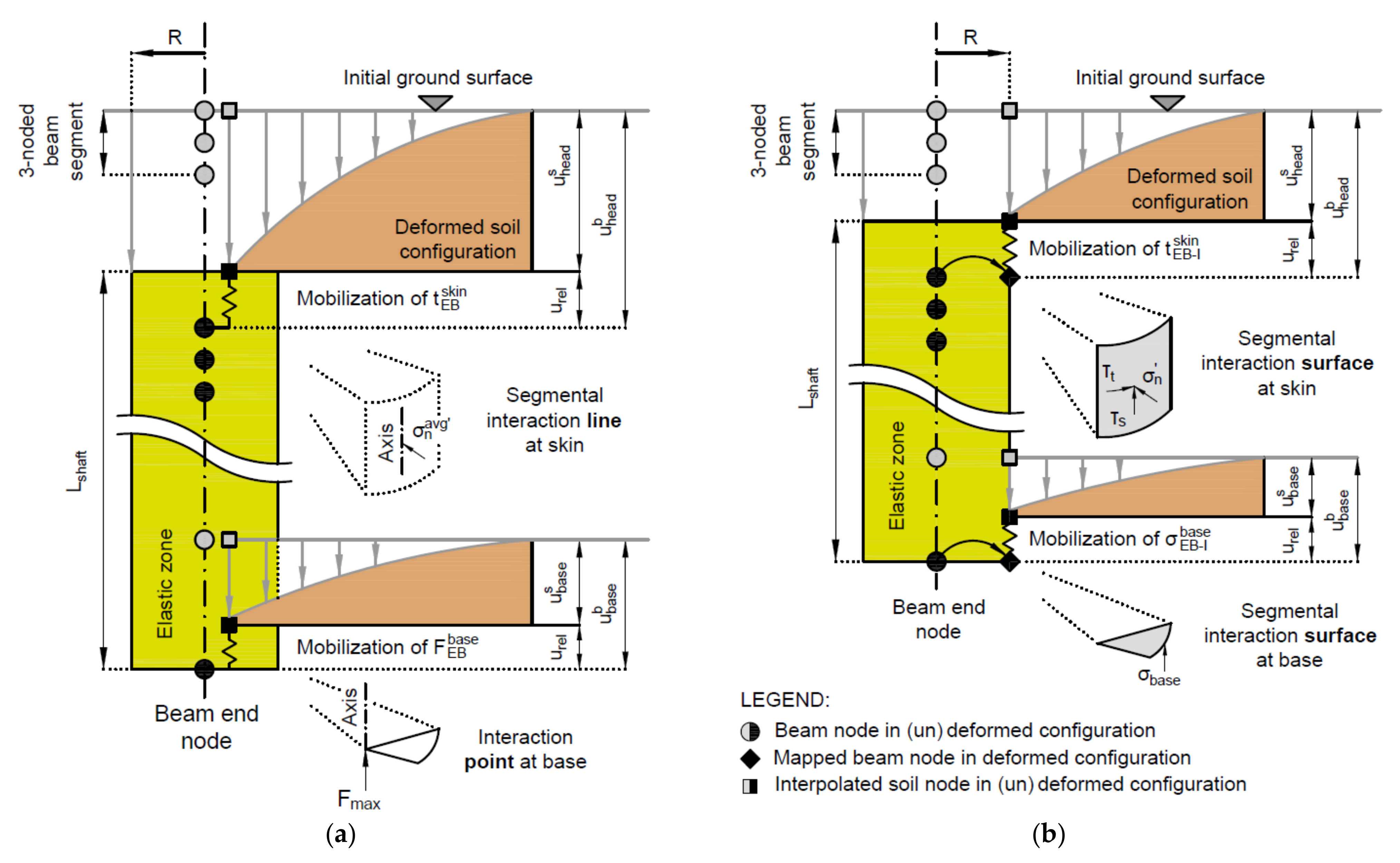
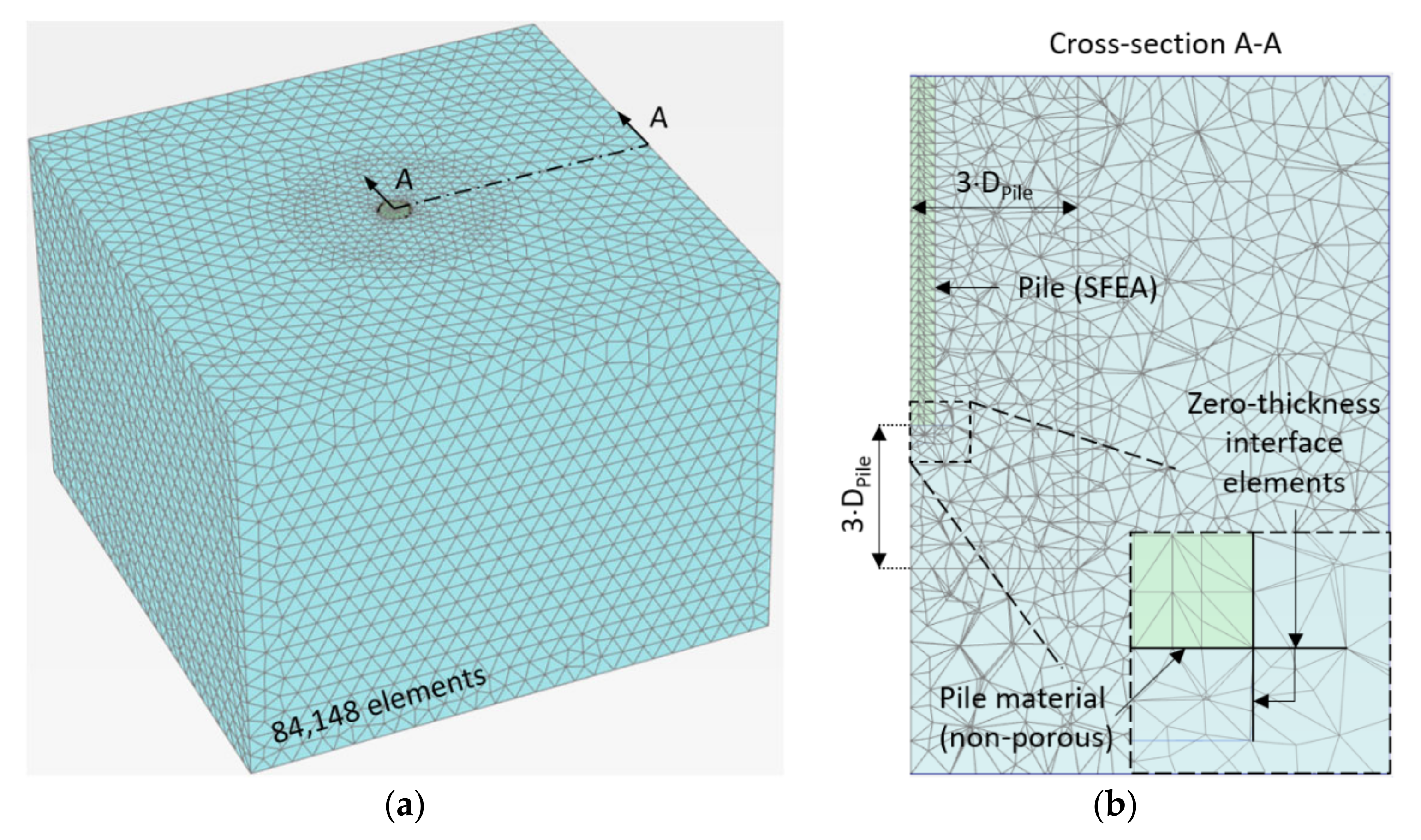
• Three-noded beam element with quadratic interpolation scheme and six DOFs (i.e., three translational DOFs, $u_x$, $u_y$, $u_z$; three rotational DOFs, ${\phi }_x$, ${\phi }_y$, ${\phi }_z$). As Timoshenko’s theory is adopted, shear deformations are explicitly taken into account. In order to improve the numerical stability in case of particularly fine mesh discretizations, an elastic zone is automatically generated in the surrounding soil. In this zone, all Gaussian points of the solid mesh are forced to remain elastic. As the zone size is controlled by the pile radius, the geometrical properties of the beam element influence the stress state in the surrounding soil [16].
• Three-noded line interfaces with the quadratic interpolation scheme and three pairs of nodes instead of single nodes, one belonging to the beam and one to the solid element in which the beam is located. This component accounts for the SSI along the shaft based on a material law that links the skin traction vector ${\mathit{t}}_{\mathit{E}\mathit{B}}^{\mathit{s}\mathit{k}\mathit{i}\mathit{n}}$ (kN/m) to the relative displacement vector ${\mathit{u}}_{\mathit{r}\mathit{e}\mathit{l}}$ (m):

  $${\mathit{u}}_{\mathit{r}\mathit{e}\mathit{l}}={\mathit{u}}^{\mathit{b}}-{\mathit{u}}^{\mathit{s}}={\mathit{N}}^{\mathit{b}}·{\mathit{a}}^{\mathit{b}}-{\mathit{N}}^{\mathit{s}}·{\mathit{a}}^{\mathit{s}}$$

  (1)

  $${\mathit{t}}_{\mathit{E}\mathit{B}}^{\mathit{s}\mathit{k}\mathit{i}\mathit{n}}={\mathit{D}}^{\mathit{e}}·{\mathit{u}}_{\mathit{r}\mathit{e}\mathit{l} }$$

  (2)

  where ${\mathit{u}}^{\mathit{b}}$ and ${\mathit{u}}^{\mathit{s}}$ (m) denote the beam and solid displacement vector, while matrices ${\mathit{N}}^{\mathit{b}}$ and ${\mathit{N}}^{\mathit{s}}$ represent the interpolation matrix, including standard Lagrangian element functions of the corresponding beam and solid elements. The elastic constitutive matrix ${\mathit{D}}^{\mathit{e}}$ (kN/m²) is composed of the embedded interface stiffnesses in normal and tangential directions. Unlike the beam component, interface stiffness matrices are evaluated employing the Newton–Cotes integration scheme, hence element function values at the nodes are either one or zero. While skin traction components in radial direction are defined as unlimited, peak values in axial direction $t_{axial,max}$ (kN/m) may be linked to the actual soil stress state using a Coulomb criterion:

  $$t_{axial, max}\le \left(c^{\prime }-{\sigma }_n^{avg\prime }·\tan {\phi }^{\prime }\right)·2·\pi ·R$$

  (3)

  where $c^{\prime }$ (kPa) and ${\phi }^{\prime }$ (°) represent the effective soil strength parameters, ${\sigma }_n^{avg\prime }$ (kPa) the averaged effective normal stress along the line interface and $R$ (m) the radius.
• Point interface with one integration point at the beam end. In its initial configuration, the latter coincides with a solid node. Similar to the line interface, SSI effects obey a material law defined in terms of ${\mathit{u}}_{\mathit{r}\mathit{e}\mathit{l}}$ (m) and the embedded foot interface stiffness $K_{base}$ (kN/m) in an axial direction. On the contrary, the ultimate tip force is limited through a user-defined tip force $F_{max}$ (kN), hence independent of the surrounding soil. Tensile stresses are internally suppressed through a tension cut-off criterion.

For details concerning virtual work considerations and the iteration procedure, the interested reader can refer to [47,48,49,50,51].

2.2. Improved Embedded Beam Formulation with Interaction Surface

To the best of found knowledge, the EB-I is yet to feature in commercial software codes. However, recent developments have been tested and incorporated in Plaxis 3D [18,42]. In order to get a better understanding of the enhancements compared to the EB, a few remarks on the implementation are noteworthy:

• Unlike EBs, which consider shaft SSI effects along the beam axis, the EB-I spreads the shaft resistance over a number of integration points located at the physical interaction surface; the same applies for SSI at the base, where the resistance is distributed over several points at the base, instead of a single point. In this way, singular stress concentrations, leading to local accumulations of plastic behaviour and large displacements along the axis, are avoided. In analogy to the EB, the skin traction vector ${\mathit{t}}_{\mathit{E}\mathit{B}-\mathit{I}}^{\mathit{s}\mathit{k}\mathit{i}\mathit{n}}$ (kN/m²) is expressed in terms of the relative displacement vector at the interaction surface ${\mathit{u}}_{\mathit{r}\mathit{e}\mathit{l}}$ (m) and the elastic stiffness matrix ${\mathit{D}}^{\mathit{e}}$ (kN/m³):

  $${\mathit{u}}_{\mathit{r}\mathit{e}\mathit{l}}={\mathit{u}}^{\mathit{b}}-{\mathit{u}}^{\mathit{s}}=\mathit{H}·{\mathit{a}}^{\mathit{b}}-{\mathit{N}}^{\mathit{s}}·{\mathit{a}}^{\mathit{s}}$$

  (4)

  $${\mathit{t}}_{\mathit{E}\mathit{B}-\mathit{I}}^{\mathit{s}\mathit{k}\mathit{i}\mathit{n}}=\frac{{\mathit{D}}^{\mathit{e}}}{2\pi \mathrm{R}}·{\mathit{u}}_{\mathit{r}\mathit{e}\mathit{l} }$$

  (5)

  where ${\mathit{u}}^{\mathit{b}}$ (m) denotes the mapped beam displacement at the interaction surface expressed in terms of the mapping matrix $\mathit{H}$ and beam nodal DOFs ${\mathit{a}}^{\mathit{b}}$. ${\mathit{u}}^{\mathit{s}}$ (m) is the solid displacement vector at the interaction surface obtained by means of interpolation, within solid elements, located at the interaction surface. The latter is calculated based on vector ${\mathit{a}}^{\mathit{s}}$ containing solid nodal DOFs and the interpolation matrix ${\mathit{N}}^{\mathit{s}}$ including standard Lagrangian element functions of the corresponding solid elements. $R$ (m) represents the beam radius and ${\mathit{D}}^{\mathit{e}}$ (kN/m²) represents the elastic stiffness matrix containing the interface stiffnesses. Since each interface element no longer poses a line, but a surface, the latter is divided by the shaft circumference. A similar approach is applied to resemble SSI at the base.
• In contrast to EBs, EB-Is are able to distinguish between two shear stress directions perpendicular to the beam axis. This allows them to enrich the slip criterion such that it accounts for any possible direction of slip failure occurring at the interaction surface:

  $${\tau }_{max}=\sqrt{{\tau }_s^2+{\tau }_t^2}\le c^{\prime }-{\sigma }_n^{\prime }·\tan {\phi }^{\prime }$$

  (6)

  where ${\tau }_{max}$ (kN/m²) is the max. local shear stress, controlled by the (perpendicularly oriented) local shear stress components ${\tau }_s$ and ${\tau }_t$ (kN/m²) acting on the interaction surface. ${\sigma }_n^{\prime }$ (kN/m²) denotes the actual normal stress developing in the surrounding soil, $c^{\prime }$ (kN/m²) and ${\phi }^{\prime }$ (°) the effective soil strength parameters. Accordingly, the intrinsic slip criterion is not restricted to the axial direction, as is the case for the EB.
• Depending on the discretization and the number of integration points at the interaction surface, the EB-I connects multiple continuum elements to one beam element. From a numerical point of view, the embedded beam stiffness is spread over a higher number of nodes, leading to relative merits in terms of global stiffness matrix conditioning (i.e., smaller difference between max. and min. diagonal terms). As a consequence, the robustness of the numerical procedure is improved compared to the EB.

For the sake of clarity, Figure 1 compares the global response of a vertically loaded single pile, modelled by means of both embedded beam formulations, namely the existing embedded beam (EB) and the improved embedded beam with interaction surface (EB-I).

3. Finite Element Modelling

3.1. Investigated Scenario and Model Description

Although single piles are rarely constructed in isolation, it is useful to consider their analysis for the numerical validation of new pile modelling methods [4]. Accordingly, the Alzey Bridge pile load test [52] serves as a reference scenario to compare the performance of the EB with the EB-I. The test program was originally intended to optimize the foundation design of a highway bridge in slightly overconsolidated Frankfurt clay. Recently, it has gained increasing popularity for the performance assessment of novel pile formulations; for example, see [16,42].

The numerical simulations, carried out in the present study, consider different pile modelling approaches and mesh discretizations. All simulations are carried out with Plaxis 3D [51]. For the sake of numerical consistency, in terms of solid element type and domain dimensions, all results are obtained using full 3D models, instead of axisymmetric 2D models or reduced 3D models for the SFEA. In view of the number of elements and DOFs required to discretize the domain, this allows for a direct comparison between SFEA and EB/EB-I models. Following the results of trial simulations, the model domain has been defined such that boundary effects are reduced to an acceptable limit; see Appendix A. Consequently, the model dimensions B_m = L_m/D_m are set to 26/19 m, which is equal to 20 and 2 times the pile diameter and length, respectively; see Figure 2a. With regard to the boundary conditions, conventional kinematic conditions are considered: a fully fixed support, with blocking of the displacements in all directions, at the lower horizontal model boundary and a horizontally fixed support with freedom of vertical displacements along lateral model boundaries. Moreover, mesh sensitivity analyses, concerning the (numerical) benchmark solution, ensure that the reference model is stable and reliable; see Appendix B.

Regardless of the pile modelling approach, the majority of the performed finite element analyses (FEA) consist of five phases. All simulations start with the definition of the initial conditions, where the initial stress field is generated by means of the K0 procedure; this is reasonable given a horizontal ground surface and homogeneous soil. The next phase concerns the pile installation; depending on the considered pile configuration, this includes the assignment of hardened concrete properties and the activation of interface elements between the pile and the surrounding soil (SFEA), or the activation of the respective embedded beam element (EB, EB-I). Hence, the piles are assumed to be homogenous in strength, stiffness, and weight, thereby ignoring effects of improper concreting [6]. According to the reference scenario, the soil around the pile is assumed to be in its initial state, which may be regarded as reasonable for non-displacement piles, where installation effects are of subordinate importance with respect to the pile behaviour [8]. Unless otherwise stated, the pile is finally subjected to displacement-driven head-down loading.

In the course of the evaluation of results, the mesh size effect on derived quantities (for example, the mobilization of skin and base resistance) is compared at different displacement levels. To satisfy practical relations on the one hand, and reduce bias on the other hand, the prescribed displacements are specified beforehand, following the L1-L2 method [53]; see Figure 2b.

Assuming drained conditions, the following prescribed displacements are determined as a function of the pile diameter ${\mathrm{D}}_{\mathrm{Pile}}$:

• $u_{L1}={\mathrm{u}}_{\mathrm{Pile}}/{\mathrm{D}}_{\mathrm{Pile}}=0.34\%$, approximating the end of the initial linear region [54].
• $u_{L2}={\mathrm{u}}_{\mathrm{Pile}}/{\mathrm{D}}_{\mathrm{Pile}}=4\%$, indicating the initiation of the final linear region [55].
• $u_{ult}={\mathrm{u}}_{\mathrm{Pile}}/{\mathrm{D}}_{\mathrm{Pile}}=10\%$, complying with the ultimate pile resistance defined in [56].

As shown in Figure 2b, $u_{L1}$ and $u_{L2}$ correspond to the pile head displacement ${\mathrm{u}}_{\mathrm{Pile}}$ at the end of the initial linear region, as well as at the initiation of the final linear region. $u_{ult}$ marks the pile head displacement at the end of loading.

3.2. Pile Modelling Approach

As suggested by [10,38,41], the numerical behaviour of embedded beam formulations is numerically validated against SFEA results (i.e., full 3D FE model). In the latter case, the swept meshing technique [57] is applied to discretize the domain with 84,148 10-noded tetrahedral elements. In this way, the solid elements representing the SFEA pile are discretized with a structured swept mesh, allowing for both a faster mesh generation process, as well as a considerable mesh size reduction compared to the default solid mesh.

In order to minimize the interpolation error associated with the mesh discretization of the model, the mesh is refined inside the pile structure, and within a zone of 3⋅${\mathrm{D}}_{\mathrm{Pile}}$ below the tip and beside the shaft, respectively; see Figure 3. To address possible occurrence of relative displacements and plastic slip parallel to the soil-structure contacts, standard zero-thickness interface elements are considered at soil-structure contacts [58,59]. The interface elements are extended beyond the physical pile boundary in order to reduce the effect of singular plasticity points developing close to the pile edge [11,60]. The interface strength is specified with a Coulomb criterion that limits the max. shear stress ${\tau }_{ max}$ (kN/m²) by

$${\tau }_{ max}=\left(c^{\prime }-{\sigma }_n^{\prime }·\tan {\phi }^{\prime }\right)·R_{inter}$$

(7)

where ${\sigma }_n^{\prime }$ (kN/m²), ${\phi }^{\prime }$ (°), and $c^{\prime }$ (kN/m²) are the effective interface normal stress, interface friction angle, and interface cohesion. In accordance with recommendations given in [61], an interface reduction factor $R_{inter}$ = 0.9 is adopted in the analyses, which represents a typical value to account for SSI between concrete piles and fine grained soils.

Contrary to SFEA interfaces, embedded interface elements are not explicitly modelled, but they are internally defined after the global mesh discretization; thus, assigning interface parameters reduces the definition of the ultimate skin and base resistance. For the sake of numerical consistency, the skin resistance is defined as layer-dependent (i.e., dependent of the stress state in the surrounding soil; see Equation (3)). In this way, the embedded interface elements are defined similarly to the interface elements used in the SFEA [12]. In an attempt to capture the SFEA pile capacity with sufficient accuracy, the base resistance is limited by the SFEA normal force developing at the pile base after the final loading step. The mesh sensitivity of both embedded beam formulations is investigated with five different mesh refinements, which are referred to as very fine, fine, medium, coarse, and very coarse (Figure 4). The model boundary conditions are specified equal to the SFEA case.

It is noted that both embedded beam formulations are analysed with the same mesh discretizations and considerably less DOFs compared to the SFEA. Since beam elements are superimposed on the solid domain, and therefore overlap the soil, the beam unit weight represents a delta unit weight to the surrounding soil [11]. Noteworthy, this differs from previous interpretations of the embedded beam unit weight documented in [27,30,31,62], where the unit weight is assigned with the actual unit weight of the volume pile; as a consequence, this approach leads to an overestimation of the soil-structure unit weight. To realistically approximate the kinematics at the pile head, the uppermost connection point is considered as free to move and rotate, relative to the surrounding soil. Additional modelling parameters summarized in

Table 2. Overview of pile parameters applied in the Alzey Bridge model.

Parameter	Symbol	Unit	SFEA		EB/EB-I 1
			Pile	Interface	Pile	Interface
Unit weight	$\gamma$	kN/m3	25.0		5.0
Young’s modulus	$E$	GPa	10.0		10.0
Poisson’s ratio	$\nu$	-	0.2
Pile diameter	$D$	m	1.3		1.3
Pile length	$L$	m	9.5		9.5
Base resistance	$F_{max}$	kN			2300.0
Interface reduction factor	$R_{inter}$	-		0.9		0.9
Effective friction angle	${\mathit{\phi }}^{\prime }$	deg		20.0		20.0
Effective cohesion	$c\prime$	kN/m2		20.0		20.0

¹ Calibrated numerical model documented in [18].

are taken from [16] and resemble on-site conditions as described in [52].

3.3. Constitutive Model and Parameter Determination

Regardless of the pile modelling approach, the use of a proper constitutive model is crucial to cover the complex stress-strain behaviour of soils. Specific to this study, this includes a realistic evolution of potential slip planes along the pile-soil contacts, which is fundamental in the analysis of the pile behaviour. Since piles may undergo a wide range of deformations, leading to considerable strains in the soil, the constitutive model should also be capable of effectively simulating the shear modulus degradation with the evolution of shear strain [63]. Lastly, the constitutive model is supposed to account for the stress dependency of soil stiffness in order to capture the gradual mobilization of skin friction with sufficient accuracy [11].

Concerning these critical modelling aspects, the Hardening Soil Small (HSS) with non-associated flow rule and small-strain stiffness overlay [64], an extension of the Hardening Soil (HS) model [65], is used in this study. While HS parameters and drainage conditions are adopted from [16], HSS-specific model parameters, namely the threshold shear strain for stiffness degradation, ${\mathsf{\gamma }}_{0.7}$, and the initial shear modulus, ${\mathrm{G}}_0$, are defined using empirical correlations documented in [66] and [67], respectively. The groundwater table is located 3.5 m below ground surface. Soil parameters adopted in the analyses are listed in

Table 3. Overview of soil parameters applied in Alzey Bridge model.

Parameter	Symbol	Unit	Value
Drainage conditions	-	-	drained
Depth of groundwater table	-	m	3.5
Unit weight	${\gamma }_{sat}$,${\gamma }_{unsat}$	kN/m3	20.0
Reference deviatoric hardening modulus at pref	$E_{50}^{ref}$	kN/m2	45,000
Reference oedometer stiffness at pref	$E_{oed}^{ref}$	kN/m2	27,150
Reference un-/reloading stiffness at pref	$E_{ur}^{ref}$	kN/m2	90,000
Power index	$m$	-	1.0
Isotropic Poisson’s ratio	${\nu }_{ur}^{\prime }$	-	0.2
Effective friction angle	${\mathit{\phi }}^{\prime }$	deg	20.0
Effective cohesion	$c^{\prime }$	kN/m2	20.0
Pre-overburden pressure	$POP$	kN/m2	50.0
Reference pressure	$p_{ref}$	kN/m2	100.0
Initial shear modulus at pref	$G_0^{ref}$	kN/m2	116,000
Threshold shear strain	${\gamma }_{0.7}$	-	0.00015

.

4. Numerical Validation

A series of finite element analyses has been performed to assess the performance of the improved embedded beam with interaction surface. Therefore, the latter is compared to the existing embedded beam formulation, as well as the SFEA, which serves as the benchmark. The simulations focus on two specific points: mesh sensitivity studies and displacements induced in the surrounding soil. In addition, practical implications are drawn based on the results.

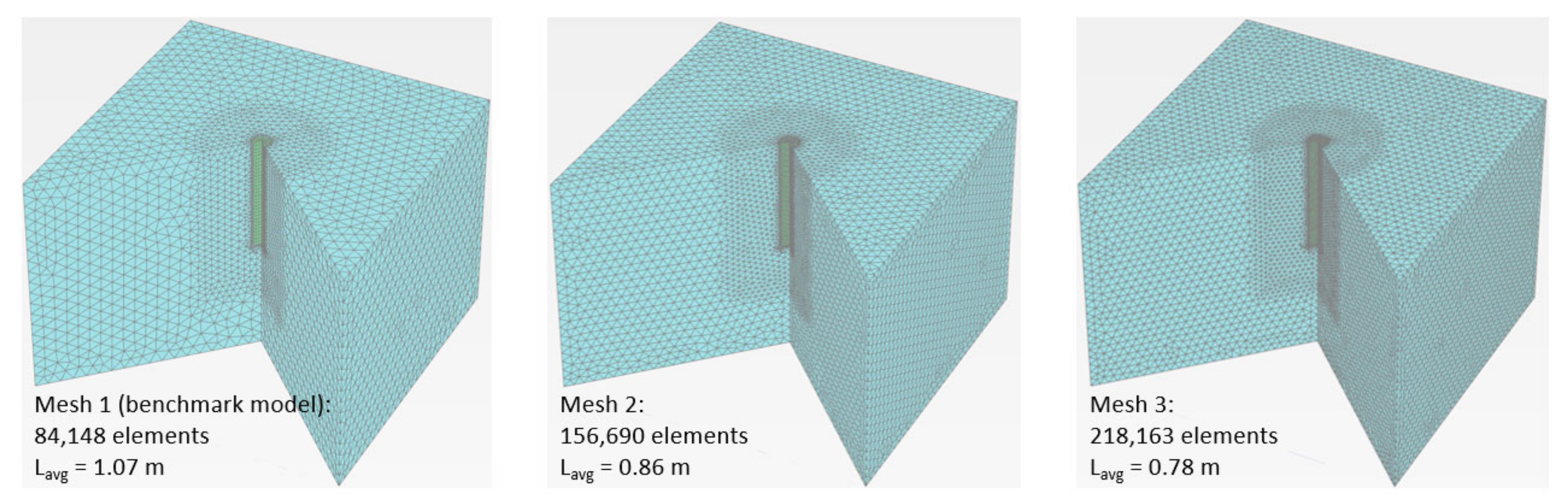
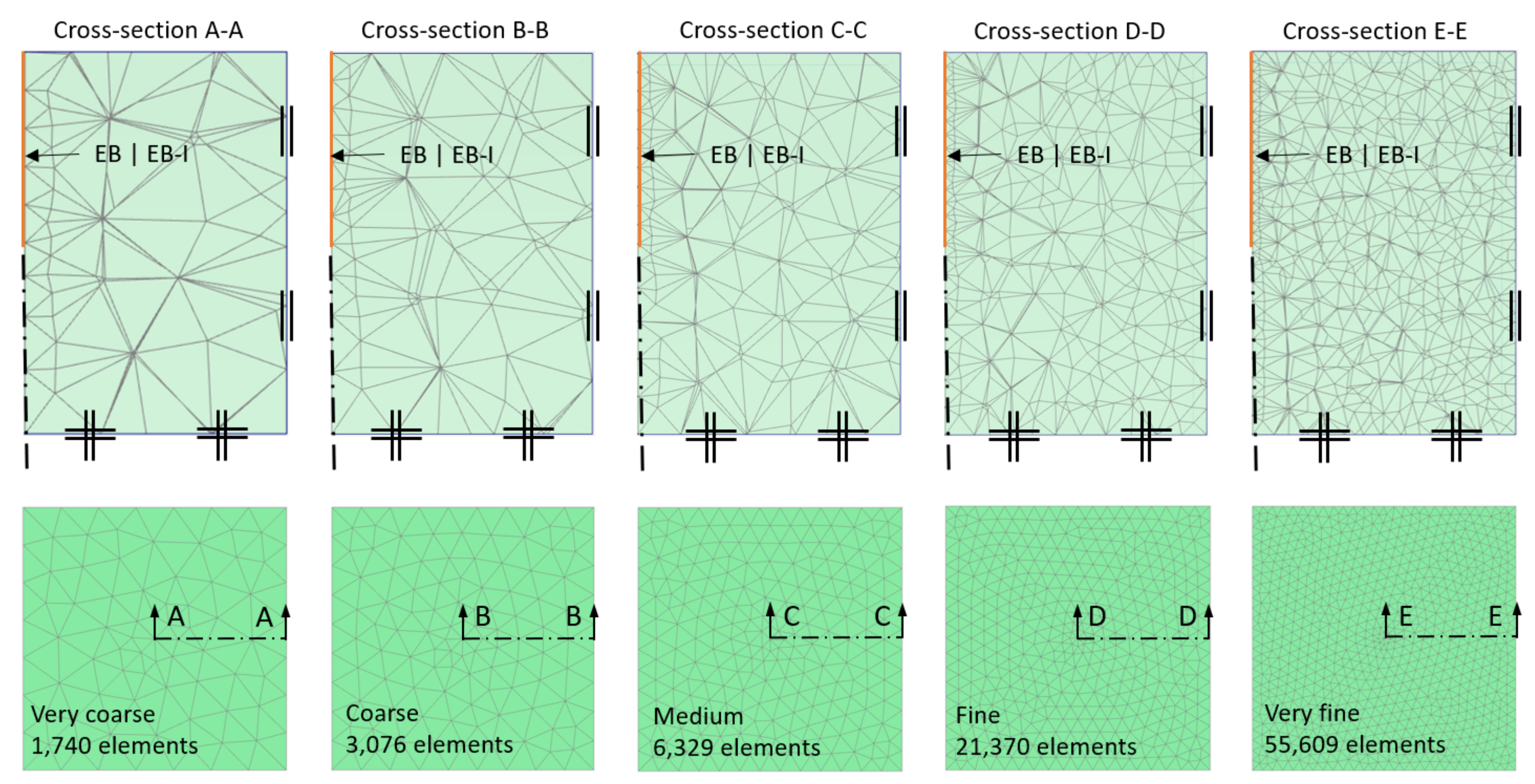
4.1. Influence of Mesh Size on Global Pile Behaviour

The most critical issue in the design of pile supported structures is a reliable prediction of the pile behaviour, in terms of bearing capacity and settlement, under working load conditions [68]. Consequently, the first series of calculations has been performed to investigate the mesh size effect on the mobilization of compressive pile resistance $R_c$ (kN).

As it can be observed in Figure 5, all pile models show a similar behaviour in the first stage of loading, regardless of spatial discretization level and pile modelling approach. However, as the load increases beyond 2000 kN, the results reveal considerable limitations of the EB, including a significant scatter of results and overestimation of bearing capacity, compared to the reference solution. Although it is generally known that coarser meshes yield a stiffer pile response, the wide scatter of load-displacement curves must be regarded as considerable obstacles to produce consistent results. In contrast, a more realistic pile response is obtained when employing the EB-I, thereby transforming the pile-soil line interface to an explicit interaction surface. Up to a relative displacement of 2%, the mobilized pile resistance magnitudes are almost independent of the domain discretization. Even at higher displacement levels, the mesh size effect remains insignificant compared to the EB.

In view of the load-displacement behaviour, the EB-I gives a softer global response compared to the EB after reaching the ultimate skin resistance, which is mainly attributed to the different mobilization of base resistance $R_b$ (kN); see Figure 6. The base–resistance curves, deduced from both embedded beam formulations, may be well approximated through bi-linear functions bounded by the max. base resistance $F_{max}$, which is a direct input to the analysis. However, the EB shows considerably steeper gradients in comparison with the EB-I, which is a direct consequence of the modified embedded base interface stiffness considered in the actual EB-I configuration. As a by-product, EB-I curves are in remarkable agreement with the reference solution. Moreover, the results confirm that the EB-I is less mesh-size dependent; for example, at a relative displacement of 2%, the range of $R_c$-values obtained with the EB-I (<100 kN) is considerably smaller when compared with the EB (>1000 kN). Nevertheless, both formulations have deficiencies regarding the initial mobilization of base resistance in the first part of loading (see Figure 6); in all cases considered, the base resistance is considerably underestimated and shows a lower mobilization rate compared to the SFEA. This must be regarded as a considerable limitation of the actual embedded beam configurations.

Figure 7 provides more insight into the effect of different mesh discretizations on the mobilization of $R_c$ at different pile displacement levels, namely $u_{L1}$, $u_{L2}$, and $u_{ult}$; see Figure 2b. The obtained $R_c$-values are normalized with respect to the benchmark solution:

$$R_{c,norm}=\frac{R_{c,EB|EB-I}}{R_{c,SFEA}}·100 \%$$

(8)

where $R_{c,norm}$ (%) is the normalized compressive pile resistance. $R_{c,EB|EB-I}$ (kN) and $R_{c,SFEA}$ (kN) represent the mobilized compressive pile resistance, either obtained with the EB, EB-I, or SFEA at a given pile head displacement. To quantify the refinement level of the considered mesh, independent of the model dimensions, the results are plotted versus the average element size $L_{avg}$ (m), which is internally controlled by the mesh coarseness factor and the model dimensions [57].

In compliance with the previous results, the EB-I achieves a satisfactory agreement with the reference solution, with the max. deviation being as little as 12%. On the contrary, $R_c$-magnitudes obtained with the EB are highly mesh-dependent. In all cases considered, the EB yields the highest $R_c$-values. In particular, for coarse mesh discretizations, the benchmark value is considerably overestimated with a peak deviation of 58%.

In order to describe the mesh size effect by means of a quantitative measure, the mesh dependency ratio $MDR$ is introduced:

$$MDR=\frac{R_{c,max}}{R_{c,min}}\ge 1.0$$

(9)

where $R_{c,max}$ and $R_{c,min}$ (kN) represent the max. and min. compressive pile resistance values obtained at a given pile head displacement, either using the EB or the EB-I. Obviously, a $MDR$ of 1.0 indicates mesh-independency, even though the results may differ from the reference solution. As expected, $MDR$-values listed in

Table 4. Summary of pile resistance values obtained at different displacement levels.

Mesh Configuration	${\mathit{L}}_{\mathit{a}\mathit{v}\mathit{g}}$	EB			EB-I			Unit
	m	${\mathit{R}}_{\mathit{c}, {\mathit{u}}_{\mathit{L}1}}$	${\mathit{R}}_{\mathit{c}, {\mathit{u}}_{\mathit{L}2}}$	${\mathit{R}}_{\mathit{c}, {\mathit{u}}_{\mathit{u}\mathit{l}\mathit{t}}}$	${\mathit{R}}_{\mathit{c}, {\mathit{u}}_{\mathit{L}1}}$	${\mathit{R}}_{\mathit{c}, {\mathit{u}}_{\mathit{L}2}}$	${\mathit{R}}_{\mathit{c}, {\mathit{u}}_{\mathit{u}\mathit{l}\mathit{t}}}$
Very coarse	4.15	2355	4642	4667	1867	3284	3855	kN
Coarse	3.44	2363	4386	4385	1877	3208	3876	kN
Medium	2.48	2045	4224	4208	1887	3017	3863	kN
Fine	1.81	1974	3723	3975	1891	3283	3916	kN
Very Fine	1.32	1940	3603	4228	1906	3071	3796	kN
	$\mathit{M}\mathit{D}\mathit{R}$	1.22	1.29	1.17	1.02	1.09	1.03	-

are remarkably smaller for the EB-I, thus underlining that the EB-I is clearly superior in the elimination of the mesh-size effect for all cases considered. For example, at the pile head displacement of $u_{L1}$, the $MDR$ reduces to 1.02 for the EB-I; at the other extreme, the $MDR$ gives 1.22 for the EB.

4.2. Influence of Mesh Size on Pile Load Transfer Mechanism

A realistic representation of the load sharing between pile shaft and pile base is critical in the analysis of geotechnical structures, including deep foundation elements. For example, Zhou et al. [69] have reported that the development of differential settlements, developing between the pile and surrounding soil, is more pronounced for end-bearing piles, in comparison with floating piles. In addition, the load-carrying mechanism influences the development of skin tractions along the pile length, hence, this is of paramount importance in the analysis of composite foundations such as piled rafts [70]. As discussed in Section 1, these structures are often modelled using EB, although the load transfer mechanism has been rarely validated in literature.

To close this knowledge gap, a closer inspection of the load separation is given in Figure 8, where relative pile head displacements are plotted versus skin resistance ratios (i.e., percentage of total load resisted by skin friction). This approach is often utilized to characterize the load-bearing behaviour of piles, whereas admissible values range from 0% (end-bearing pile) to 100% (floating pile). In all cases considered, the results infer that the skin resistance ratio decreases with increasing pile displacement, albeit underestimated, at around 20%, in the initial stage of loading. While all curves obtained with the EB-I converge to the reference solution at approximately 40%, the EB indicates mesh sensitive values that vary within higher bounds. This observation complies with previous findings concerning $R_c$ [42]; as the ultimate base resistance is limited by $F_{max}$, the scatter of magnitudes must be caused by an overestimation of the skin resistance. This tendency, in turn, is presumably triggered by singular skin traction values developing near the pile base, which are likely to occur due to a combination of very high stress gradients in the soil elements around the pile base and constitutive models concerning stress-dependent soil stiffness; a comprehensive discussion on this limitation inherent to EBs is provided in [11].

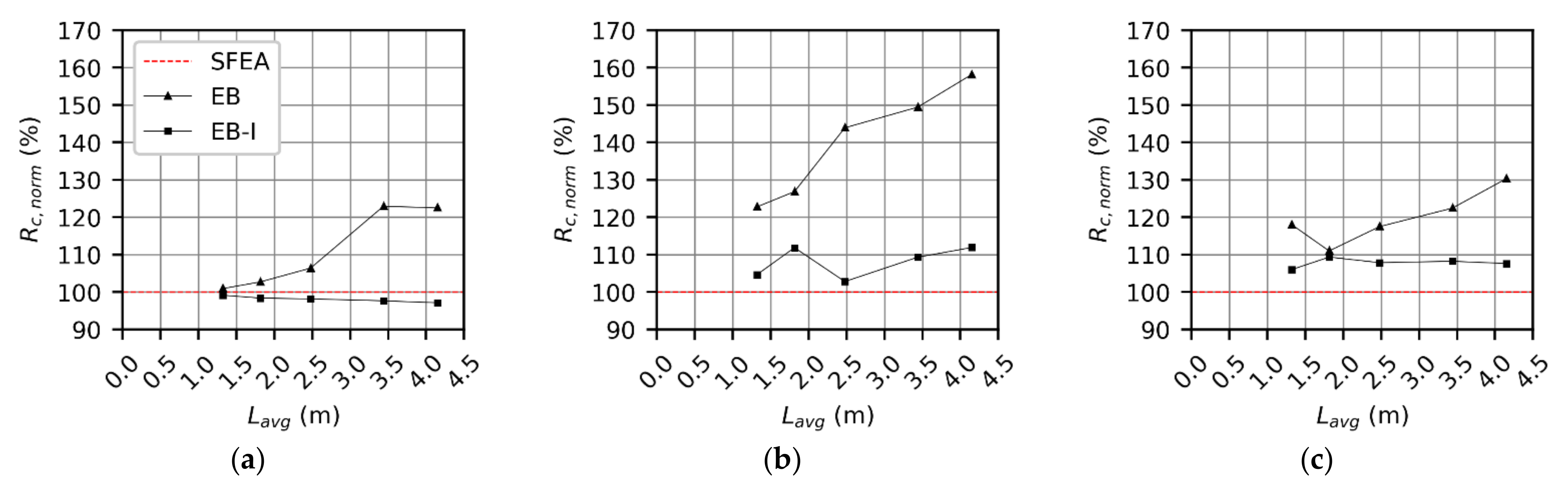
4.3. Influence of Mesh Size on Pile Stiffness Coefficient

In traditional serviceability analysis of pile-plate systems, SSI effects are numerically considered as spring constants acting on bending plates [56]. In this context, the pile stiffness coefficient $k_s$(MN/m), representing the pile stiffness, is expressed by the formula:

$$k_s=\frac{R_{c,i}}{u_i}$$

(10)

where $R_{c,i}$ (kN) is the compressive pile resistance, mobilized at the pile head displacement $u_i$ (mm). The current engineering approach assumes $k_s$ from the secant on the resistance-settlement curve of pile load tests working in the initial linear region, commonly adopting empirical data with respect to allowable settlements [69]. Following engineering practice, $k_s$ is calculated as the slope of the secant line connecting the origin to the curve at $u_{L2}$; see Figure 3b. Figure 9a presents $k_s$-values as a function of $L_{avg}$; in analogy to Equation (8), derived quantities are normalized with respect to the benchmark solution. As one can observe, all EB-I results are in remarkable agreement with the benchmark solution; on the contrary, the EB overestimates $k_s$ up to 26%. With regard to the mesh dependency ratio, the EB-I yields values that are too small to warrant differentiation, while the EB, again, indicates a notable mesh sensitivity; see Figure 9b. From a practical point of view, the EB-I increases the confidence with which $k_s$ may be estimated by reducing the influence of the mesh size.

4.4. Influence of Mesh Size on Mobilization of Skin Traction

Many researchers have focused on the evaluation of normal forces to study the load-transfer mechanism of EB along the pile length (for example, see [13,24,37]). Skin traction profiles, in contrast, have received only subordinate attention. The underlying cause becomes apparent from Figure 10, which compares both approaches at typical working load conditions. Regardless of the pile modelling approach, the normal force distribution indicates a smooth distribution of skin tractions along the pile length. In comparison with the reference solution, increasing deviations towards the pile base are attributed to the spurious mobilization of base resistance, which is underestimated with the EB and EB-I in the initial stage of loading; see Section 4.1.

In contrast, the EB yields numerical oscillations in the predicted skin traction response for all mesh discretizations considered, even though the mean values are almost identical to the benchmark results. To explain the origin for this abnormality, the following points deserve attention:

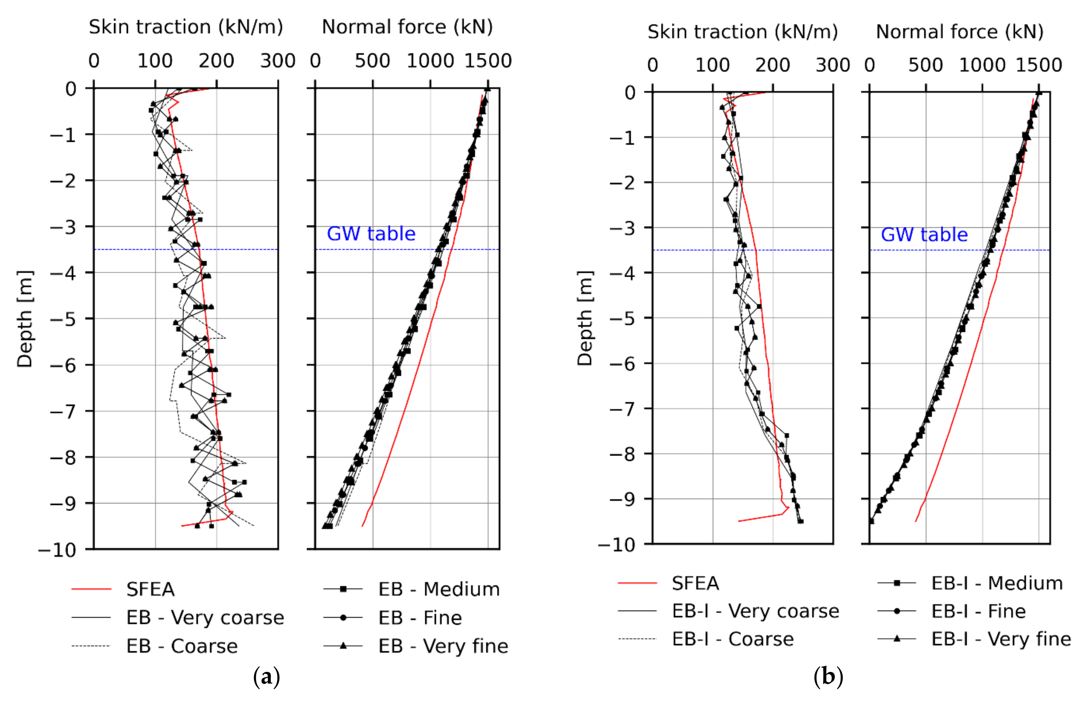
• EB results of the beam and the line interface are presented at the nodes [71]. Therefore, the normal forces are internally extrapolated from Gaussian beam stress points to the node of interest, leading to smooth profiles. In contrast, Equation (2) is used to work out nodal skin tractions, which are consequently a function of the relative displacement vector field and the embedded stiffness matrix. An additional parametric study (not shown) has revealed that skin traction oscillations also occur with linear elastic soil behaviour, ensuring identical (stress-independent) embedded stiffness values along the pile length. Consequently, the apparent reasoning of the oscillations must be attributed to the relative displacement vector field, which is interpolated using displacement vector fields of different continuity at the element boundaries (C0 for soil displacements; C1 for beam displacements).
• The spurious tendency to produce oscillations is amplified by high stress and strain gradients, predominantly occurring at the EB axis. Since the EB-I evaluates the relative displacements at multiple points over the real pile perimeter, instead of one point located at the pile axis, local effects are significantly reduced. As a consequence, skin traction profiles are considerably smoothened.
• Oscillations of integration point stresses, observed with the SFEA, are caused by steep stress gradients at the pile ends. This was already explained in [58].

In view of skin traction analysis, previous observations demonstrate that the EB-I poses a significant enhancement compared to the EB, as it significantly reduces numerical inconsistencies leading to unrealistic oscillations in skin traction.

4.5. Displacements Induced in Surronding Soil

In design situations, where the cost-effectiveness of pile caps are of primary interest, pile spacings should be kept as close as possible [68]. The optimal pile layout, however, should also ensure the effectiveness of resisting piles, which is primarily achieved through sufficiently large pile spacings [72]. The assessment of optimal pile spacings may be based on the evaluation of settlement profiles at different pile depths [52]. Moreover, mixed foundations, involving deep foundation elements, must satisfy serviceability limits, defined in terms of admissible differential settlements [73]. In any of these cases, it is important to realistically capture spatial soil displacements induced by external loads. An insight into the predicted displacement behaviour can be gained by looking at Figure 11, where the final distribution of soil settlements, induced by a vertical load of 1500 kN, are illustrated. At a first glance, it can be observed that:

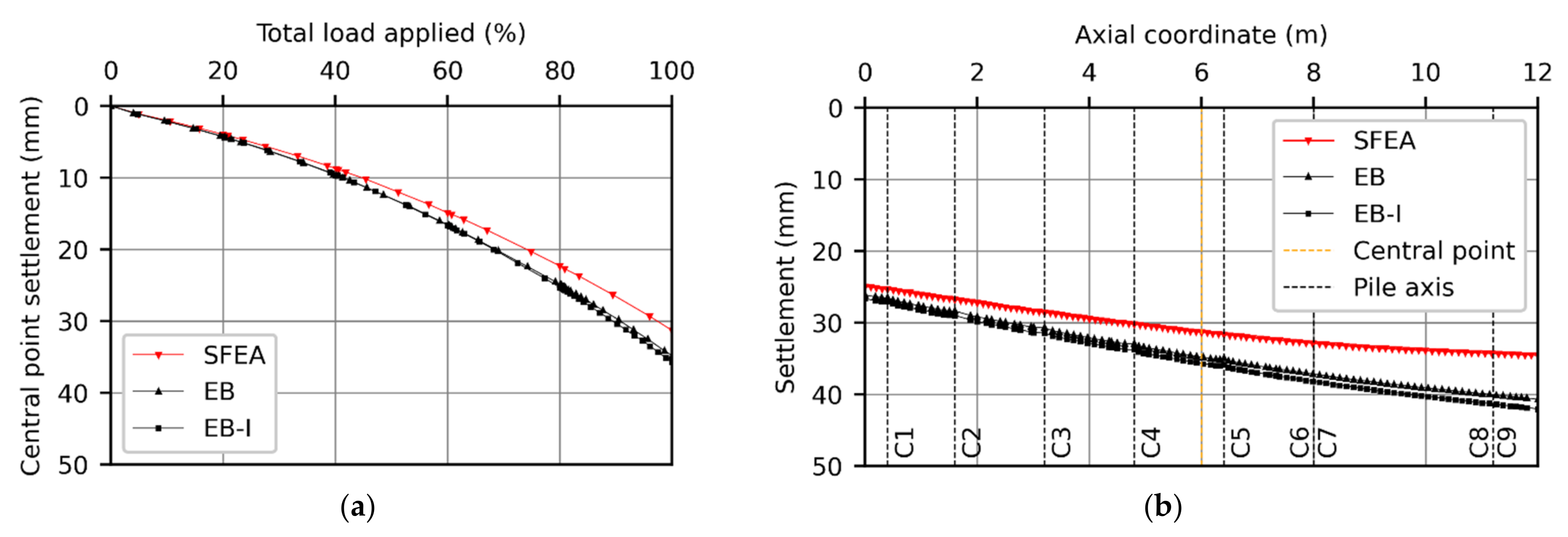
• Except for the displacement field in close proximity to the pile base, all calculations yield similar results within the soil domain (i.e., zone ${\mathsf{\Omega }}_1$).
• Apparently, the pile domain (i.e., zone ${\mathsf{\Omega }}_2$) experiences settlement concentrations, which are particularly pronounced for the EB. This is a direct consequence of the SSI considered along a line, thereby introducing high displacement gradients in a radial direction. In contrast, the EB-I finds homogenous displacement regions of lower magnitude enclosed by the explicit interaction surface; although vertical displacements are slightly underestimated compared to the SFEA, the EB-I is obviously superior to the EB with regard to the prediction of the general deformation pattern inside ${\mathsf{\Omega }}_2$.

A closer inspection of the settlement profiles, at different pile depths, reveals the apparent origin of previous observations (see Figure 12): With the SFEA, an explicit interface (i.e., series of linked pairs of nodes) is inserted at the physical pile-soil contact. This interface fulfils the role of a kinematic discontinuity, capable of accounting for extremely high strain gradients [74]. Concerning both embedded beam formulations, the fallacy to account for the displacement jump at the pile skin becomes obvious. This is due to the implicit nature of the embedded interface, where displacement jumps are internally considered to describe the nodal connectivity of beam and soil nodes, but do not evolve in the physical mesh.

From an engineering perspective, the settlement curves evolving outside the pile domain vary within acceptable bounds; at a distance greater than two times the pile diameter, the settlement profiles of all pile modelling approaches practically coincide. On the contrary, increasing deviations are observed towards the pile axis. While the EB tends to overestimate the settlements, the EB-I gives lower values. In all cases considered, peak deviations are observed at the lowermost settlement profile (EB: −54%, EB-I: 54%). Further improvements of the spatial deformation behaviour are mainly related to the stiffness definition of the embedded interface, which is at the forefront of ongoing research.

5. Case Study

As part of the restructuring of the Vienna rail node, Tschuchnigg [11] has described the application of 3D finite element simulations to the foundation design of central station “Wien Mitte”; see Figure 13. Due to serviceability requirements, critical zones of the existing slab are supported by jet-grout columns to satisfy serviceability criterions, mainly concerning differential settlements.

The performance of previously described embedded beam formulations is assessed by performing the same numerical simulations. In absence of measurement data, the results are, again, numerically validated against a full 3D representation of the problem including SFEA, which is widely recognized as convenient for the numerical analysis of similar problems; for example, see [75,76]. By taking advantage of the symmetry, the model size is defined as 50 × 4 × 48 m; see Figure 14a. The soil layering is similar to the real project. The raft of the simplified model is supported by nine jet-grout columns, which are symmetrically arranged on the foundation axis; see Figure 14b. SSI between soil and raft boundaries are addressed by means of zero-thickness interface elements [58,59] (not shown). The base model boundary condition is defined as fully fixed, whereas the vertical boundaries are set to allow vertical movement of soil layers (i.e., roller supports). Depending on the column modelling approach, the domain is discretized with 102,811 (SFEA) and 41,205 (EB, EB-I) 10-noded tetrahedral elements with quadratic element function.

Table 5. Overview of HSS soil parameters used in the analyses (Wien Mitte).

Parameter	Symbol	Unit	Gravel	Sandy Silt I|II	Sand	Stiff Silt
Depth of groundwater table	-	m	6.0	-	-	-
Layer thickness	$t$	m	8.0	3.0|11.0	14.0|2.0	10.0
Unit weight	${\gamma }_{sat},{\gamma }_{unsat}$	kN/m3	21.5|21.0	20.0	21.0|20.0	20.0
Reference deviatoric hardening modulus at pref	$E_{50}^{ref}$	kN/m2	40,000	20,000	25,000	30,000
Reference oedometer stiffness at pref	$E_{oed}^{ref}$	kN/m2	40,000	20,000	25,000	30,000
Reference un-/reloading stiffness at pref	$E_{ur}^{ref}$	kN/m2	120,000	50,000	62,500	90,000
Power index	$m$	-	0.0	0.8	0.65	0.6
Isotropic Poisson’s ratio	${\nu }_{ur}^{\prime }$	-	0.2	0.2	0.2	0.2
Effective friction angle	${\mathit{\phi }}^{\prime }$	deg	35.0	27.5	32.5	27.5
Effective cohesion	$c\prime$	kN/m2	0.1	20.0|30.0	5.0	30.0
Ultimate dilatancy angle	$\Psi$	deg	5.0	0.0	2.5	0.0
Pre-overburden pressure	$POP$	kN/m2	600	600	600	600
Reference pressure	$p^{ref}$	kN/m2	100	100	100	100
Initial shear modulus at pref	$G_0^{ref}$	kN/m2	138,000	81,000	93,000	116,000
Threshold shear strain	${\gamma }_{0.7}$	-	0.00015	0.00015	0.00015	0.00015

gives the HSS soil parameters adopted in the analyses; in analogy to Section 3.3, HSS-specific soil parameters are obtained using profound empirical correlations [66,67]. Additional material parameters related to the column-raft system, as well as the calculation phase sequence, are described in [11].

Figure 15a compares the load-settlement curves, obtained with the embedded beam models, against the benchmark solution. It is interesting to note that settlements occurring at the central point (see Figure 14) are practically coincident (<1 mm) up to an applied load of around 40%. Beyond this value, one can observe slightly higher settlements for both embedded beam models, presumably due to lower base resistance mobilization rates in the initial stage of loading; see Section 4.1. The settlement profiles, illustrated in Figure 15b, indicate that this tendency is further amplified towards edge columns 8 and 9, which are exposed to a higher surface load. At final load, corresponding edge settlements are 35 mm (SFEA), 41 mm (EB), and 42 mm (EB-I).

Figure 16a indicates the displacements of the foundation at the final loading stage. Following the definition documented in [73], the displacements along the foundation axis are expressed as the tangent rotation $\theta$ (i.e., negative when the tangent of successive nodes points downwards). Again, almost identical results are calculated for both embedded beam formulations. Ignoring the presence of successive peak values, the derived foundation movements appear to be in reasonable agreement with the reference solution. Successive peak values, however, are an important aspect in structural analysis (especially for the design of the raft) and thus, require discussion. In the simulations, all column-raft contacts are imposed with a rigid connection. While the reference solution spreads the column-raft interaction over multiple nodes, both embedded beam formulations consider the column-raft connection at one node only. As the raft is discretized with solid elements occupying no rotational DOFs, the connection type reduces to a hinge for single-node connections, which has a remarkable influence on the magnitude of the tangent rotation developing in direction of the foundation axis.

Figure 16b illustrates the observed deformation patterns schematically. In the reference model, the tangent rotation achieves max. values outside the column-raft contacts, indicating offsets between the columns. Since the tangent rotations are purely negative in sign, the tangent between successive nodes (in direction of the axial coordinate) points strictly downwards. In contrast, tangent rotation peak values evolve at the column-raft contacts with the EB and EB-I. In addition, the tangent rotations vary in sign at the column-raft contacts, indicating relatively high curvatures. Taking into account the bending moment–curvature relationship, this is likely to result in the spurious prediction of internal forces and an inconvenient raft design. To circumvent these obstacles, a more realistic representation of foundation movement could be realized by using alternative modelling techniques such as the hybrid modelling approach described by Lődör and Balázs [24], where embedded beams are circumscribed by volume elements at connection areas.

The last section is devoted to examining the load sharing between members of the composite geotechnical structure. In this context, the column raft coefficient ${\alpha }_{cr}$ at different loading stages is calculated as:

$${\alpha }_{cr}=\frac{\sum R_{column}}{R_{total}}$$

(11)

where $\sum R_{column}$ (kN) defines the sum of loads carried by the columns and $R_{total}$ (kN) the total load applied. Figure 17a depicts ${\alpha }_{cr}$ as a function of relative load applied. All models show higher ${\alpha }_{cr}$-values with increasing load level, indicating that additional load portions are predominantly carried by the columns. On the one hand, both embedded beam formulations show almost identical results and converge to ${\alpha }_{cr}$ = 0.46 after the final stage of loading. On the other hand, deviations compared to the benchmark are striking (${\alpha }_{cr}$ = 0.71) and require discussion.

To study the load transfer characteristics in more detail, Figure 17b shows the normal force distribution along (central) column 5. Obviously, arising differences with regard to ${\alpha }_{cr}$ can be attributed to a combination of remaining issues associated with both embedded beam configurations, namely:

• At load levels, fairly below the ultimate skin resistance, the load carried by the base resistance is significantly underestimated; see Section 4.1. As a consequence, the general column response is too soft.
• The single-node connection causes a combination of unrealistic settlement concentrations and spurious stress path evolutions in the vicinity of column-raft contacts. As a result, column 5 experiences negative skin friction along the upper portion of the shaft (normal force increases up to a depth of around 1.0 m), instead of a direct pile head load. As a consequence, lower ${\alpha }_{cr}$-values are obtained.

More research, with the aim of analysing complex boundary value problems, is part of ongoing research.

6. Discussion and Conclusions

Two different embedded beam formulations for finite element modelling of deep foundation elements have been extensively compared in terms of geotechnical and structural performance, namely the embedded beam element (EB) and the recently developed embedded beam element with interaction surface (EB-I). Derived quantities are numerically validated against the widely accepted standard FE approach (SFEA), a full 3D representation of respective structures. To the authors’ knowledge, this work poses the first attempt to assess the suitability of the EB-I for practical use. In this respect, a number of critical aspects have been tackled, such as load sharing between base and shaft, evolution of soil displacements in the surrounding soil, and mobilization of skin resistance. In this context, particular emphasis has been given to the influence of the mesh sensitivity of results. The following conclusions are drawn from the FEA of deep foundation elements:

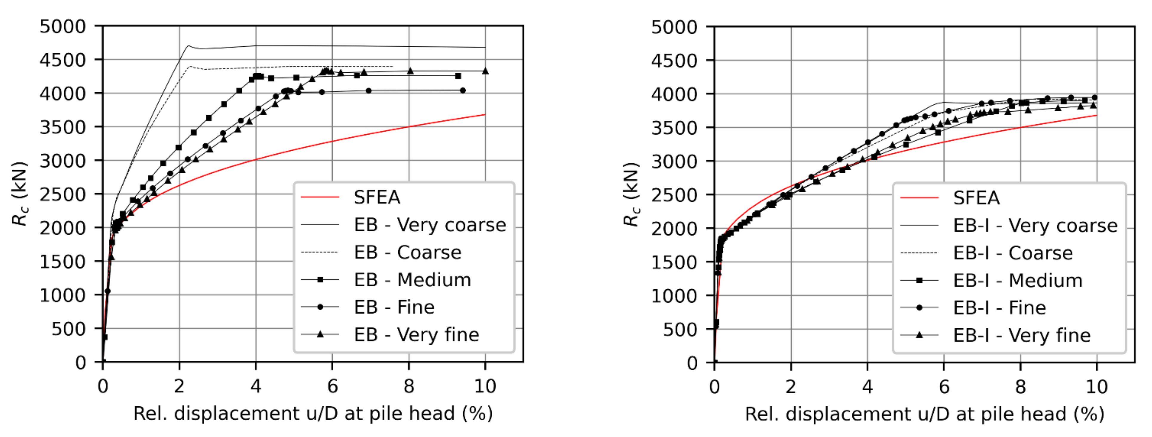
• In the initial phase of loading, both embedded beam formulations yield load-displacement responses which are in remarkable agreement with the SFEA. At load levels beyond the shaft capacity, load-displacement curves obtained with the EB are considerably mesh sensitive, whereas the pile behaves stiffer with increasing mesh-coarseness. The EB-I, in contrast, reduces the mesh size effect tremendously. Moreover, the EB-I achieves a satisfactory agreement with the SFEA.
• Concerning the predicted pile capacity, the EB produces a wide scatter of results which must be regarded as unsatisfactory. This shortcoming is effectively eliminated by the EB-I; in all cases considered, the pile capacity varies, within acceptable bounds, slightly higher than the SFEA target value. Reducing the mesh size effect also allows engineers to deduce pile stiffness coefficients with more confidence.
• At typical working load conditions, skin traction profiles obtained with both embedded beam formulations fit SFEA results qualitatively well. However, the EB produces numerical oscillations about the mean that are significantly reduced with the EB-I.
• Although both embedded beam formulations appear to capture the evolution of spatial soil displacements with sufficient accuracy, major differences occur inside the pile domain. While the EB calculates the highest soil displacement at the pile axis, the EB-I computes almost constant displacement profiles within the pile boundaries, as is the case with the SFEA. However, reproducing displacement jumps at the pile skin lies beyond the capabilities of the actual EB-I configuration.
• When modelling deep foundation elements of composite structures, by means of embedded beams, the connection of the individual structures needs to be considered carefully: specifically, if embedded beams are imposed with a rigid connection. Otherwise, the prediction of structural forces, shaft-base load sharing, and differential settlements may lack physical meaning.

Considering the above findings, the EB-I proves superior to the EB. Nevertheless, several limitation of the current version have been observed which require further research effort. This includes the development of a generally applicable concept capable of predicting SSI effects at the base with sufficient accuracy; in addition, guidelines concerning the definition of the ultimate base resistance are still in demand. Further, future studies should explore whether the elastic zone approach is still required with the EB-I. In the course of this paper, the application of EB-Is was limited to axial loading cases, neglecting passive, as well as lateral, loading; therefore, future studies should focus on more complex loading situations, whereas the credibility of results should be carefully validated using measurement data. Research to resolve remaining issues is ongoing with promising results so far.

References

1. Maheshwari, B.K.; Watanabe, H. Nonlinear Dynamic Behavior of Pile Foundations: Effects of Separation at the Soil-Pile Interface. Soils Found 2006, 46, 437–448. [Google Scholar] [CrossRef] [Green Version]
2. Poulos, H.G.; Davis, E.H. Pile Foundation Analysis and Design, 1st ed.; Poulos, H.G., Davis, E.H., Eds.; Wiley: New York, NY, USA, 1980; ISBN 0471020842. [Google Scholar]
3. von Wolffersdorff, P.-A.; Henke, S. Möglichkeiten und Grenzen numerischer Methoden in der Geotechnik. Bautechnik 2021, 98, 1–17. [Google Scholar] [CrossRef]
4. Potts, D.M.; Zdravkovic, L. Finite Element Analysis in Geotechnical Engineering: Application, 1st ed.; Thomas Telford Ltd.: London, UK, 2001; ISBN 0727728121. [Google Scholar]
5. Engin, H.K. Modelling of Installation Effects: A Numerical Approach. Ph.D. Thesis, Delft University of Technology, Delft, The Netherlands, 2013. [Google Scholar]
6. Schmüdderich, C.; Shahrabi, M.M.; Taiebat, M.; Lavasan, A.A. Strategies for numerical simulation of cast-in-place piles under axial loading. Comput. Geotech. 2020, 125, 1–19. [Google Scholar] [CrossRef]
7. Wehnert, M.; Vermeer, P.A. Numerische Simulation von Probebelastungen an Großbohrpfählen. In Proceedings of the Bauen in Boden und Fels: 4. Kolloquium, Ostfildern, Germany, 20–21 January 2004; TAE: Esslingen, Germany, 2004; pp. 555–565, ISBN 3924813558. [Google Scholar]
8. Han, F.; Salgado, R.; Prezzi, M.; Lim, J. Shaft and base resistance of non-displacement piles in sand. Comput. Geotech. 2017, 83, 184–197. [Google Scholar] [CrossRef]
9. Chen, Y.-J.; Lin, S.-S.; Chang, H.-W.; Marcos, M.C. Evaluation of side resistance capacity for drilled shafts. J. Mar. Sci. Technol. 2011, 19, 210–221. [Google Scholar] [CrossRef]
10. Turello, D.F.; Sánchez, P.J.; Blanco, P.J.; Pinto, F. A variational approach to embed 1D beam models into 3D solid continua. Comput. Struct. 2018, 206, 145–168. [Google Scholar] [CrossRef]
11. Tschuchnigg, F. 3D Finite Element Modelling of Deep Foundations Employing an Embedded Pile Formulation. Ph.D. Thesis, Graz University of Technology, Graz, Austria, 2013. [Google Scholar]
12. Tschuchnigg, F.; Schweiger, H.F. The embedded pile concept—Verification of an efficient tool for modelling complex deep foundations. Comput. Geotech. 2015, 63, 244–254. [Google Scholar] [CrossRef]
13. Tradigo, F.; Pisanò, F.; Di Prisco, C. On the use of embedded pile elements for the numerical analysis of disconnected piled rafts. Comput. Geotech. 2016, 72, 89–99. [Google Scholar] [CrossRef]
14. Ninić, J.; Stascheit, J.; Meschke, G. Beam-solid contact formulation for finite element analysis of pile-soil interaction with arbitrary discretization. Int. J. Numer. Anal. Meth. Geomech. 2014, 38, 1453–1476. [Google Scholar] [CrossRef]
15. Sadek, M.; Shahrour, I. A three dimensional embedded beam element for reinforced geomaterials. Int. J. Numer. Anal. Meth. Geomech. 2004, 28, 931–946. [Google Scholar] [CrossRef]
16. Engin, H.; Brinkgreve, R.; Septanika, E. Improved embedded beam elements for the modelling of piles. In Numerical Models in Geomechanics, Proceedings of the 10th International Symposium on Numerical Models in Geomechanics, Rhodes, Greece, 25–27 April 2007; Pande, G.N., Ed.; Taylor & Francis: London, UK, 2007; ISBN 978-0-415-44027-1. [Google Scholar]
17. Oliveria, D.; Wong, P.K. Use of embedded pile elements in 3D modelling of piled-raft foundations. Aust. Geomech. J. 2011, 46, 9–19. [Google Scholar]
18. Smulders, C.M. An Improved 3D Embedded Beam Element with Explicit Interaction Surface. Master’s Thesis, Delft University of Technology, Delft, The Netherlands, 2018. [Google Scholar]
19. Ukritchon, B.; Faustino, J.C.; Keawsawasvong, S. Numerical investigations of pile load distribution in pile group foundation subjected to vertical load and large moment. Geomech. Eng. 2016, 10, 577–598. [Google Scholar] [CrossRef]
20. Engin, H.K.; Brinkgreve, R.B.J. Investigation of Pile Behaviour Using Embedded Piles. In Proceedings of the 17th International Conference on Soil Mechanics and Geotechnical Engineering, Alexandria, Egypt, 5–9 October 2009; Hamza, M., Shahien, M., El-Mossallamy, Y., Eds.; IOS Press: Amsterdam, The Netherlands, 2009; pp. 1189–1192. [Google Scholar]
21. Jongpradist, P.; Haema, N.; Lueprasert, P. Influence of pile row under loading on existing tunnel. In Tunnels and Underground Cities: Engineering and Innovation Meet Archaeology, Architecture and Art; Peila, D., Viggiani, G., Celestino, T., Eds.; CRC Press: London, UK, 2019; pp. 5711–5719. ISBN 9781003031857. [Google Scholar]
22. Engin, H.; Septanika, E.; Brinkgreve, R. Estimation of Pile Group Behavior using Embedded Piles. In Proceedings of the 12th International Conference on Computer Methods and Advances in Geomechanics, Goa, India, 1–6 October 2008; Jadhav, M.N., Ed.; Curran: New York, NY, USA, 2008. ISBN 9781622761760. [Google Scholar]
23. Engin, H.; Brinkgreve, R.; Bonnier, P.; Septanika, E. Modelling piled foundation by means of embedded piles. In Geotechnics of Soft Soils: Focus on Ground Improvement, Proceedings of the 2nd International Workshop, Glasgow, Scotland, 3–5 September 2008; Karstunen, M., Leoni, M., Eds.; Taylor & Francis: London, UK, 2008; pp. 131–136. ISBN 978-0-415-47591-4. [Google Scholar]
24. Lődör, K.; Balázs, M. Finite element modelling of rigid inclusion ground improvement. In Numerical Methods in Geotechnical Engineering, Proceedings of the 9th European Conference on Numerical Methods in Geotechnical Engineering, Porto, Portugal, 25–27 June 2018; Cardoso, A.S., Borges, J.L., Costa, P.A., Gomes, A.T., Marques, J.C., Vieira, C.S., Eds.; CRC Press: London, UK, 2018; pp. 1–8. ISBN 9781138544468. [Google Scholar]
25. Tschuchnigg, F.; Schweiger, H.F. Numerical study of simplified piled raft foundations employing an embedded pile formulation. In Proceedings of the 1st International Symposium on Computational Geomechanics. ComGeo I, Juan-les-Pins, France, 29 April–1 May 2009; IC2E: Rhodes, Greece, 2009; pp. 743–752. [Google Scholar]
26. Lee, S.W.; Cheang, W.; Swolfs, W.M.; Brinkgreve, R. Modelling of piled rafts with different pile models. In Numerical Methods in Geotechnical Engineering, Proceedings of 7th European Conference on Numerical Methods in Geotechnical Engineering, Trondheim, Norway, 2–4 June 2010; Benz, T., Nordal, S., Eds.; CRC Press: London, UK, 2010; pp. 1–6. ISBN 9780429206191. [Google Scholar]
27. Elshehahwy, E.R.; Eltahrany, A.; Dif, A. Numerical Analysis Validation Using Embedded Pile. In Advances in Numerical Methods in Geotechnical Engineering, Proceedings of 2nd GeoMEast International Congress and Exhibition on Sustainable Civil Infrastructures, Cairo, Egypt, 10–15 November 2019; Shehata, H., Desai, C.S., Eds.; Springer: Berlin/Heidelberg, Germany, 2019; pp. 199–208. ISBN 978-3-030-01925-9. [Google Scholar]
28. Watcharasawe, K.; Jongpradist, P.; Kitiyodom, P.; Matsumoto, T. Measurements and analysis of load sharing between piles and raft in a pile foundation in clay. Geomech. Eng. 2021, 24, 559–572. [Google Scholar] [CrossRef]
29. Banerjee, R.; Bandyopadhyay, S.; Sengupta, A.; Reddy, G.R. Settlement behaviour of a pile raft subjected to vertical loadings in multilayered soil. Geomech. Geoengin. 2020, 1–15. [Google Scholar] [CrossRef]
30. Abbas, Q.; Kim, G.; Kim, I.; Kyung, D.; Lee, J. Lateral Load Behavior of Inclined Micropiles Installed in Soil and Rock Layers. Int. J. Geomech. 2021, 21, 1–13. [Google Scholar] [CrossRef]
31. Abbas, Q.; Choi, W.; Kim, G.; Kim, I.; Lee, J. Characterizing uplift load capacity of micropiles embedded in soil and rock considering inclined installation conditions. Comput. Geotech. 2021, 132, 1–12. [Google Scholar] [CrossRef]
32. El-Sherbiny, M.M.; El-Sherbiny, R.M.; El-Mamlouk, H. Three Dimensional Effect of Grouted Discontinuous Berms for Passive Support of Diaphragm Walls. In Proceedings of the Grouting 2017: Jet Grouting, Diaphragm Walls, and Deep Mixing, Honolulu, HI, USA, 9–12 July 2017; Gazzarrini, P., Richards, J.T.D., Bruce, D.A., Byle, M.J., El Mohtar, C.S., Johnsen, L.F., Eds.; American Society of Civil Engineers: Reston, VA, USA, 2017; pp. 571–583, ISBN 9780784480809. [Google Scholar]
33. Marjanović, M.; Vukićević, M.; König, D.; Schanz, T.; Schäfer, R. Modeling of laterally loaded piles using embedded beam elements. In Contemporary Achievements in Civil Engineering, Proceedings of 4th International Conference, Subotica, Serbia, 22–23 April 2016; Faculty of Civil Engineering: Novi Sad, Serbia, 2016; pp. 349–358. [Google Scholar]
34. Abo-Youssef, A.; Morsy, M.S.; El Ashaal, A.; El Mossallamy, Y.M. Numerical modelling of passive loaded pile group in multilayered soil. Innov. Infrastruct. Solut. 2021, 6, 1–13. [Google Scholar] [CrossRef]
35. Al-abboodi, I.; Sabbagh, T.T. Numerical Modelling of Passively Loaded Pile Groups. Geotech. Geol. Eng. 2019, 37, 2747–2761. [Google Scholar] [CrossRef] [Green Version]
36. Scarfone, R.; Morigi, M.; Conti, R. Assessment of dynamic soil-structure interaction effects for tall buildings: A 3D numerical approach. Soil Dyn. Earthq. Eng. 2020, 128, 1–14. [Google Scholar] [CrossRef]
37. Di Prisco, C.; Flessati, L.; Porta, D. Deep tunnel fronts in cohesive soils under undrained conditions: A displacement-based approach for the design of fibreglass reinforcements. Acta Geotech. 2020, 15, 1013–1030. [Google Scholar] [CrossRef]
38. Ninic, J. Computational Strategies for Predictions of the Soil-Structure Interaction during Mechanized Tunneling. Ph.D. Thesis, Ruhr University Bochum, Bochum, Germany, 2015. [Google Scholar]
39. Granitzer, A.; Tschuchnigg, F.; Summerer, W.; Galler, R.; Stoxreiter, T. Construction of a railway tunnel above the main drainage tunnel of Stuttgart using the cut-and-cover method. Bauingenieur 2021, 96, 156–164. [Google Scholar] [CrossRef]
40. Lo, S. A study in an attempt to use embedded pile structure elements to simulate soil nail structures in PLAXIS 2D 2012 and 3D 2012. In Numerical Methods in Geotechnical Engineering, Proceedings of the 8th European Conference on Numerical Methods in Geotechnical Engineering, Delft, The Netherlands, 18–20 June 2014; Hicks, M., Brinkgreve, R., Rohe, A., Eds.; CRC Press: London, UK, 2014; pp. 765–769. ISBN 978-1-138-00146-6. [Google Scholar]
41. Turello, D.F.; Pinto, F.; Sánchez, P.J. Embedded beam element with interaction surface for lateral loading of piles. Int. J. Numer. Anal. Meth. Geomech. 2016, 40, 568–582. [Google Scholar] [CrossRef]
42. Smulders, C.M.; Hosseini, S.; Brinkgreve, R. Improved embedded beam with interaction surface. In Proceedings of the 17th European Conference on Soil Mechanics and Geotechnical Engineering, Reykjavík, Iceland, 1–6 September 2019; Sigursteinsson, H., Erlingsson, S., Bessason, B., Eds.; COC: Reykjavík, Iceland, 2019; pp. 1048–1055. [Google Scholar]
43. Turello, D.F.; Pinto, F.; Sánchez, P.J. Three dimensional elasto-plastic interface for embedded beam elements with interaction surface for the analysis of lateral loading of piles. Int. J. Numer. Anal. Meth. Geomech. 2017, 41, 859–879. [Google Scholar] [CrossRef]
44. Turello, D.F.; Pinto, F.; Sánchez, P.J. Analysis of lateral loading of pile groups using embedded beam elements with interaction surface. Int. J. Numer. Anal. Meth. Geomech. 2019, 43, 272–292. [Google Scholar] [CrossRef] [Green Version]
45. Jauregui, R.; Silva, F. Numerical Validation Methods. In Numerical Analysis—Theory and Application; Awrejcewicz, J., Ed.; InTech: Toyama, Japan, 2011; ISBN 978-953-307-389-7. [Google Scholar]
46. Oberkampf, W.L.; Trucano, T.G.; Hirsch, C. Verification, validation, and predictive capability in computational engineering and physics. Appl. Mech. Rev. 2004, 57, 345–384. [Google Scholar] [CrossRef] [Green Version]
47. Ferreira, D.; Manie, J. DIANA—Finite Element Analysis: DIANA Documentation—Release 10.4. Available online: https://dianafea.com/manuals/d104/Diana.html (accessed on 25 February 2021).
48. Truty, A.; Zimmermann, T.; Podles, K.; Obrzud, R. ZSOIL.PC 2020: User Manual—Theory. Available online: https://www.zsoil.com/zsoil_manual/TM-Man.pdf (accessed on 26 July 2021).
49. Rocscience Online Help: Online Documentation. Available online: https://www.rocscience.com/about (accessed on 25 February 2021).
50. FLAC3D 7.0 Documentation. Available online: http://docs.itascacg.com/flac3d700/common/sel/doc/manual/sel_manual/piles/piles.html?node903 (accessed on 26 February 2021).
51. PLAXIS Scientific Manual: 3D—Connect Edition V21. Available online: https://communities.bentley.com/cfs-file/__key/communityserver-wikis-components-files/00-00-00-05-58/PLAXIS3DCE_2D00_V21.01_2D00_04_2D00_Scientific.pdf (accessed on 26 July 2021).
52. Sommer, H.; Hambach, P. Großpfahlversuche im Ton für die Talbrücke Alzey. Bauingenieur 1974, 49, 310–317. [Google Scholar]
53. Hirany, A.; Kulhawy, F.H. Interpretation of Load Tests on Drilled Shafts—Part 1: Axial Compression. In Proceedings of the Foundation Engineering—Current Principles and Practices, Evanston, IL, USA, 25–29 June 1989; Kulhawy, F.H., Ed.; American Society of Civil Engineers: New York, NY, USA, 1989; pp. 1132–1149, ISBN 0872627047. [Google Scholar]
54. Chen, Y.-J.; Fang, Y.-C. Critical Evaluation of Compression Interpretation Criteria for Drilled Shafts. J. Geotech. Geoenvironmental Eng. 2009, 135, 1056–1069. [Google Scholar] [CrossRef]
55. Hirany, A.; Kulhawy, F.H. On the Interpretation of Drilled Foundation Load Test Results. In International Deep Foundations Congress, Proceedings of the Deep Foundations: An International Perspective on Theory, Design, Construction, and Performance, Orlando, FL, USA, 14–16 February 2002; O’Neill, M.W., Townsend, F.C., Eds.; American Society of Civil Engineers: New York, NY, USA, 2002; pp. 1018–1028. ISBN 9780784406014. [Google Scholar]
56. German Geotechnical Society. Recommendations on Piling (EA-Pfähle), 2nd ed.; Wilhelm Ernst & Sohn: Berlin, Germany, 2014; ISBN 9783433030189. [Google Scholar]
57. PLAXIS Reference Manual: 3D—Connect Edition V21. Available online: https://communities.bentley.com/cfs-file/__key/communityserver-wikis-components-files/00-00-00-05-58/PLAXIS3DCE_2D00_V21.01_2D00_02_2D00_Reference.pdf (accessed on 16 August 2021).
58. Day, R.A.; Potts, D.M. Zero thickness interface elements—Numerical stability and application. Int. J. Numer. Anal. Meth. Geomech. 1994, 18, 689–708. [Google Scholar] [CrossRef]
59. Goodman, R.; Taylor, R.; Brekke, T. A Model for the Mechanics of Jointed Rock. J. Soil Mech. Found. Div. 1968, 94, 637–659. [Google Scholar] [CrossRef]
60. van Langen, H.; Vermeer, P.A. Interface elements for singular plasticity points. Int. J. Numer. Anal. Meth. Geomech. 1991, 15, 301–315. [Google Scholar] [CrossRef]
61. Kulhawy, F.H. Limiting tip and side resistance: Fact or Fallacy? In Proceedings of the Analysis and Design of Pile Foundations, San Francisco, CA, USA, 1–5 October 1984; Meyer, J.R., Ed.; American Society of Civil Engineers: New York, NY, USA, 1984; pp. 80–98. [Google Scholar]
62. Sheil, B.; McCabe, B.A. Predictions of friction pile group response using embedded piles in PLAXIS. In Proceedings of the 3rd International Conference on New Developments in Soil Mechanics and Geotechnical Engineering, Nicosia, Turkey, 28–30 June 2012; Near East University: Nicosia, Turkey, 2012; pp. 679–686. [Google Scholar]
63. Fleming, W.G.K.; Weltman, A.; Randolph, M.F.; Elson, K. Piling Engineering, 3rd ed.; Taylor & Francis: London, UK, 2020; ISBN 9780367659387. [Google Scholar]
64. Benz, T.; Schwab, R.; Vermeer, P. Small-strain stiffness in geotechnical analyses. Bautechnik 2009, 86, 16–27. [Google Scholar] [CrossRef]
65. Schanz, T.; Vermeer, P.A.; Bonnier, P.G. The hardening soil model: Formulation and verification. In Beyond 2000 in Computational Geotechnics, 1st ed.; Brinkgreve, R.B.J., Ed.; Routledge: London, UK, 2019; pp. 281–296. ISBN 9781315138206. [Google Scholar]
66. Vucetic, M.; Dobry, R. Effect of Soil Plasticity on Cyclic Response. J. Geotech. Eng. 1991, 117, 89–107. [Google Scholar] [CrossRef]
67. Alpan, I. The geotechnical properties of soils. Earth-Sci. Rev. 1970, 6, 5–49. [Google Scholar] [CrossRef]
68. Viggiani, C.; Mandolini, A.; Russo, G. Piles and Pile Foundations, 1st ed.; Taylor & Francis: London, UK, 2012; ISBN 978-0-415-49066-5. [Google Scholar]
69. Urbonas, K.; Slizyte, D.; Mackevicius, R. Influence of the pile stiffness on the ground slab behaviour. J. Civ. Eng. Manag. 2016, 22, 690–698. [Google Scholar] [CrossRef]
70. Hanisch, J.; Katzenbach, R.; König, G. (Eds.) Kombinierte Pfahl-Plattengründungen; Ernst & Sohn: Berlin, Germany, 2001; ISBN 3433016062. [Google Scholar]
71. Schreppers, G.-J. Bond-slip Reinforcements and Pile Foundations. Available online: https://dianafea.com/sites/default/files/2018-04/Bondslip_reinforcements_and_Pile_foundations.pdf (accessed on 26 July 2021).
72. Schmidt, H.-H.; Buchmaier, R.F.; Vogt-Breyer, C. Grundlagen der Geotechnik, 5th ed.; Springer Fachmedien Wiesbaden: Wiesbaden, Germany, 2017; ISBN 978-3-658-14930-7. [Google Scholar]
73. British Standards Institution. BS EN 1997-1:2004: Eurocode 7: Geotechnical Design—Part 1: General Rules; BSI: London, UK, 2004. [Google Scholar]
74. de Gennaro, V.; Frank, R.; Said, I. Finite element analysis of model piles axially loaded in sands. Riv. Ital. Geotec. 2008, 2, 44–62. [Google Scholar]
75. Cho, J.; Lee, J.-H.; Jeong, S.; Lee, J. The settlement behavior of piled raft in clay soils. Ocean Eng. 2012, 53, 153–163. [Google Scholar] [CrossRef]
76. Poulos, H.G. Piled raft foundations: Design and applications. Géotechnique 2001, 51, 95–113. [Google Scholar] [CrossRef]
77. Benz, T. Small-Strain Stiffness of Soils and Its Numerical Consequences. Ph.D. Thesis, University of Stuttgart, Stuttgart, Germany, 2007. [Google Scholar]
Figure 1. Global response of an axially loaded pile, considered by means of different modelling approaches: (a) embedded beam (EB); (b) embedded beam with interaction surface (EB-I). In both cases, the mobilization of skin tractions is primarily controlled by the relative displacement vector u r e l   (“spring”) and the slip criterion (“friction element”).
Processes 09 01739 g001
Figure 2. (a) Model geometry, boundary conditions, and (b) characteristic load-displacement regions after [53].
Processes 09 01739 g002
Figure 3. (a) 3D view of global SFEA mesh; (b) cross-sectional view of SFEA mesh detail.
Processes 09 01739 g003
Figure 4. Mesh discretizations considered for EB/EB-I models.
Processes 09 01739 g004
Figure 5. Influence of spatial discretization on mobilization of compressive pile resistance.
Processes 09 01739 g005
Figure 6. Influence of spatial discretization on the mobilization of base resistance.
Processes 09 01739 g006
Figure 7. Influence of spatial discretization on the mobilization of pile resistance at different displacement levels, namely (a) u L 1 , (b) u L 2 , (c) u r e l   .
Processes 09 01739 g007
Figure 8. Influence of spatial discretization on load separation plotted by means of skin resistance ratio.
Processes 09 01739 g008
Figure 9. Mesh size effect on (a) normalized pile stiffness factor and (b) respective mesh dependency ratio.
Processes 09 01739 g009
Figure 10. Influence of mesh size on development of skin traction and normal force distribution in an axial direction at a vertical load of 1500 kN: (a) EB, (b) EB-I.
Processes 09 01739 g010
Figure 11. Settlement contour plots at a vertical load of 1500 kN: (a) SFEA, (b) EB, (c) EB-I. The latter models are obtained with the fine mesh configuration. The real pile skin is indicated by dashed lines.
Processes 09 01739 g011
Figure 12. (a) Settlement profiles and (b) vertical settlements at the pile axis, obtained with a vertical load of 1500 kN at different pile depths.
Processes 09 01739 g012
Figure 13. Project overview “Wien Mitte”.
Processes 09 01739 g013
Figure 14. Description of the FE analysis model “Wien Mitte”: (a) Model configuration and (b) side/3D view of pile-raft system.
Processes 09 01739 g014
Figure 15. (a) Central point settlement plotted as a function of total load applied and (b) settlement curve along the foundation axis at final load, obtained with SFEA, EB, and EB-I.
Processes 09 01739 g015
Figure 16. (a) Foundation movement at peak load and (b) schematic illustration of deformation patterns obtained with different column modelling approaches.
Processes 09 01739 g016
Figure 17. (a) Column raft coefficient and (b) normal force distribution developing along column 5, plotted as a function of total load applied.
Processes 09 01739 g017