Experimental and Numerical Investigation of the Air Side Heat Transfer of a Finned Tubes Heat Exchanger

Abstract

The heat transfer was experimentally and numerically studied in this article. Characteristics of circular fins over a bent tube at different tube orientations and air velocities were investigated, and then compared with analytical results from the literature. For the experimental investigation, a simple setup was compiled inside of a wind tunnel, where the velocity and the inlet temperature of the air; the volume flow rate; and the inlet and outlet temperatures of the water were measured. Three different orientations were investigated with the set-up: the bent tube in line with the air flow with the same and opposite water inlet positions, and the bent tube perpendicular to the air flow. According to the results, the position has a significant effect on the heat transfer coefficient. A numerical study was also performed in accordance with the measurements in ANSYS-CFX computational fluid dynamics (CFD) software. The results of the CFD showed an acceptable correlation with the results of measurement; however, the results of analytical calculation from the literature show a significant discrepancy; the calculated heat performance is only about one-third of the measured values. This article presents the steps of measurement, simulation and analytical calculations, and shows solution possibilities in the calculation of the air-side heat transfer functions.

1. Introduction

Heat exchangers have been the most widely used equipment in chemical, energy and food industrial fields. The convective form of heat transfer is used in them, so several factors have significant effects on the performance. Thus, research, modeling and simulation of heat transfer processes and the search of optimization opportunities are essential for increasing performance. One large group of these devices, made up of the finned tube heat exchangers, plays important roles in several industrial processes, particularly wherein gas is one of the heat exchange media. The use of these fins with different geometries can significantly increase the heat transfer surface.

The shapes, sizes and orientations of the fins can be extremley varied. Review articles present the most common cases. Basavarajappa et al. [1] and Bhuiyan and Islam [2] provide general summaries; Pongsoi et al. [3] shows up the flow characteristics and heat transfer properties of the spiral shaped fins; and Unger et al. [4] shows the same properties for oval tubes with novel fins. Chai and Tassou [5] made a very thorough summary. A large body of literature has been developed based on vortex generators with different fins. The results were summarized in two ways. On the one hand, based on representative experimental investigations; on the other hand, based on representative numerical studies, similarly to Sheikholeslami et al. [6]. It is also very important to clarify the flow conditions when studying the heat transfer process. The position of the investigated fins in the direction of air flow can result in significant differences in heat performance. Unger et al. [7] demonstrated by measurements that the greater the angle at which the fins form with the air flow, the higher the Nu number; thus, developing the heat transfer coefficient and increasing the distance between the fins has the same effect.

An up-to date approach to the combined increase of the air-side heat transfer coefficient and the heat transfer surface using spiral or wavy fins was investigated by Peng [8], Syuhada et al. [9] and Wang et al. [10]. Their results show that the value of the resulting heat transfer coefficient does not necessarily increase with decreasing fin pitch. Fins that are too close already have an adverse effect on the coefficient, but still represent a much higher value than in a case without fins. Of course, other considerations may play a role in the selection of the fin type. Some of these are the aspects related to the assembly. Bhale et al. [11] investigated the performances of the H-type finned tube banks and different material savings, and surface enhancement options were compared by computational fluid dynamics (CFD) analysis. It is also possible to investigate the compact heat exchangers, as investigated by Moorthy et al. [12].

Applying computational fluid dynamics (CFD) software is essential for operational design. In case of finned tube heat exchangers, the emphasis is not on the examination of water-side heat transfer coefficient. These tubes are circular or elliptical cross-section tubes in most cases, and it is more expedient to test with simpler external heat transfer cases. The resulting air-side heat transfer coefficient in this case depends most on the geometry used. However, in a lot of design cases, an experimental model cannot be built for every geometry because it would cost a lot of time and money. CFD software has a huge advantage since all kinds of geometry can be examined in the virtual environment. These results can be used to make empirical correlations to the given geometry that are essential, for example, in an optimization process [13]. Experimental Nu number correlations can be developed for newer heat exchangers using CFD software. Taler et al. [14] determined new air side Nusselt numbers for each row of plate fin and tube heat exchangers.

Many researchers are studying the flow around the fins. Petrik et al. [15] investigated the flow pattern between squared fins. To reduce the computational demand, the volume bounded by the fins was replaced with a porous medium. Another important aspect is the application of the appropriate turbulence model. Nemati and Moghomi [16] showed in their study the differences that can be caused by using different turbulence models. Mon et al. [17] investigated inline and staggered arrangements of tubes. The conclusion is that the heat transfer coefficient will be higher in the case of a higher fin pitch and fin height ratio. The heat transfer is independent if this ratio is equal to a 0.32 coefficient.

2. Experimental Setup and Measurement

2.1. Experimental Setup and Devices

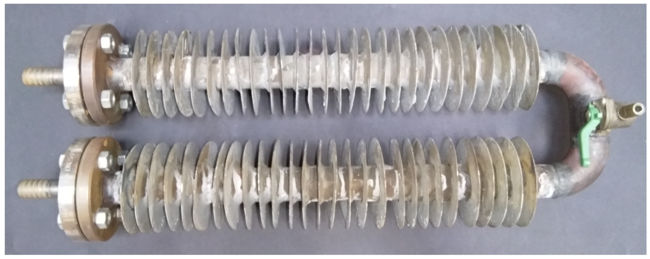
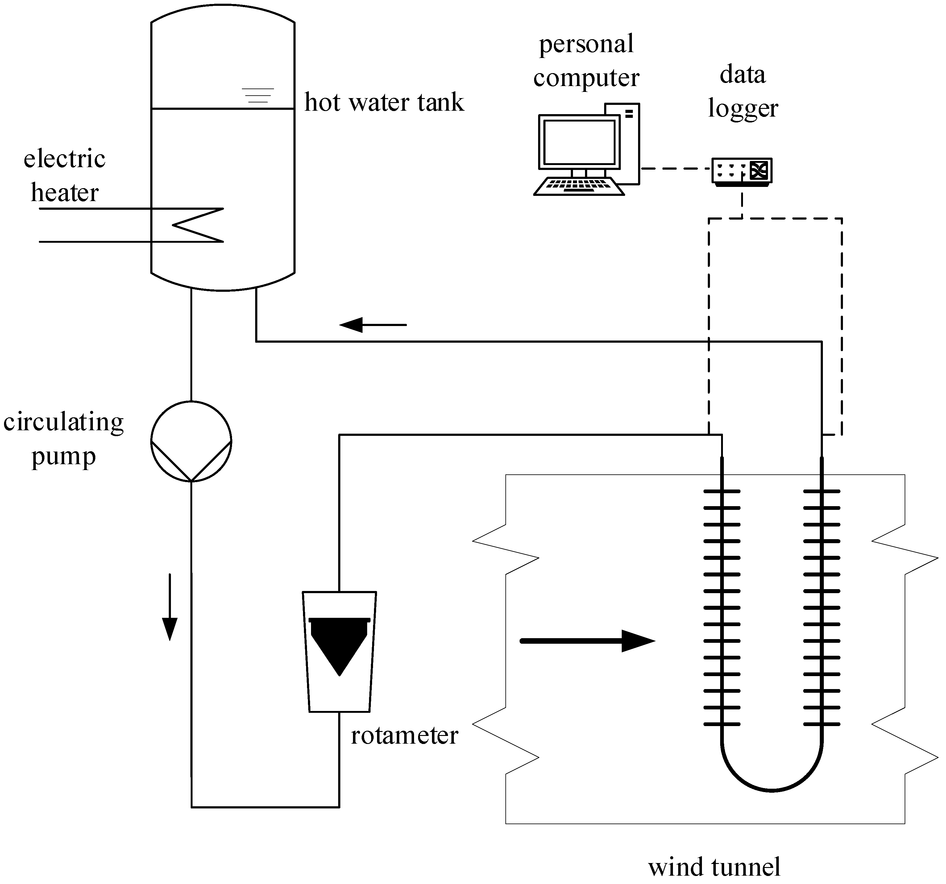
The investigated finned tube heat exchanger shown in Figure 1. The 80-l hot water tank heated by electricity produces and stores the hot fluid. The hot fluid was water, and its temperature was 60 ${}^{\circ }$C. This hot fluid is circulated by a pump in a 3/4${}^{″}$ hoses and flows through a rota-meter, which detects the volume flow rate. After the rotameter fluid goes through the heat exchanger. Exiting the heat exchanger, the cooled liquid returns to the water tank. The experimental setup is shown in Figure 2.

The tube register was placed in a wind tunnel. A Quantum X type MX1609 thermocouple amplifier with type K thermocouples was used for data collection. Two temperatures were measured: the inlet and outlet temperatures of the heat exchanger with 5 Hz sampling rate. Data processing was done with catman^® Easy software (2006 by Hottinger Baldwin Messtechnik GmbH, Darmstad, Germany).

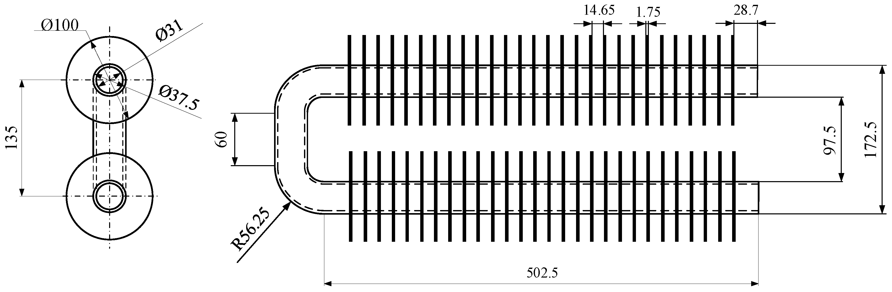
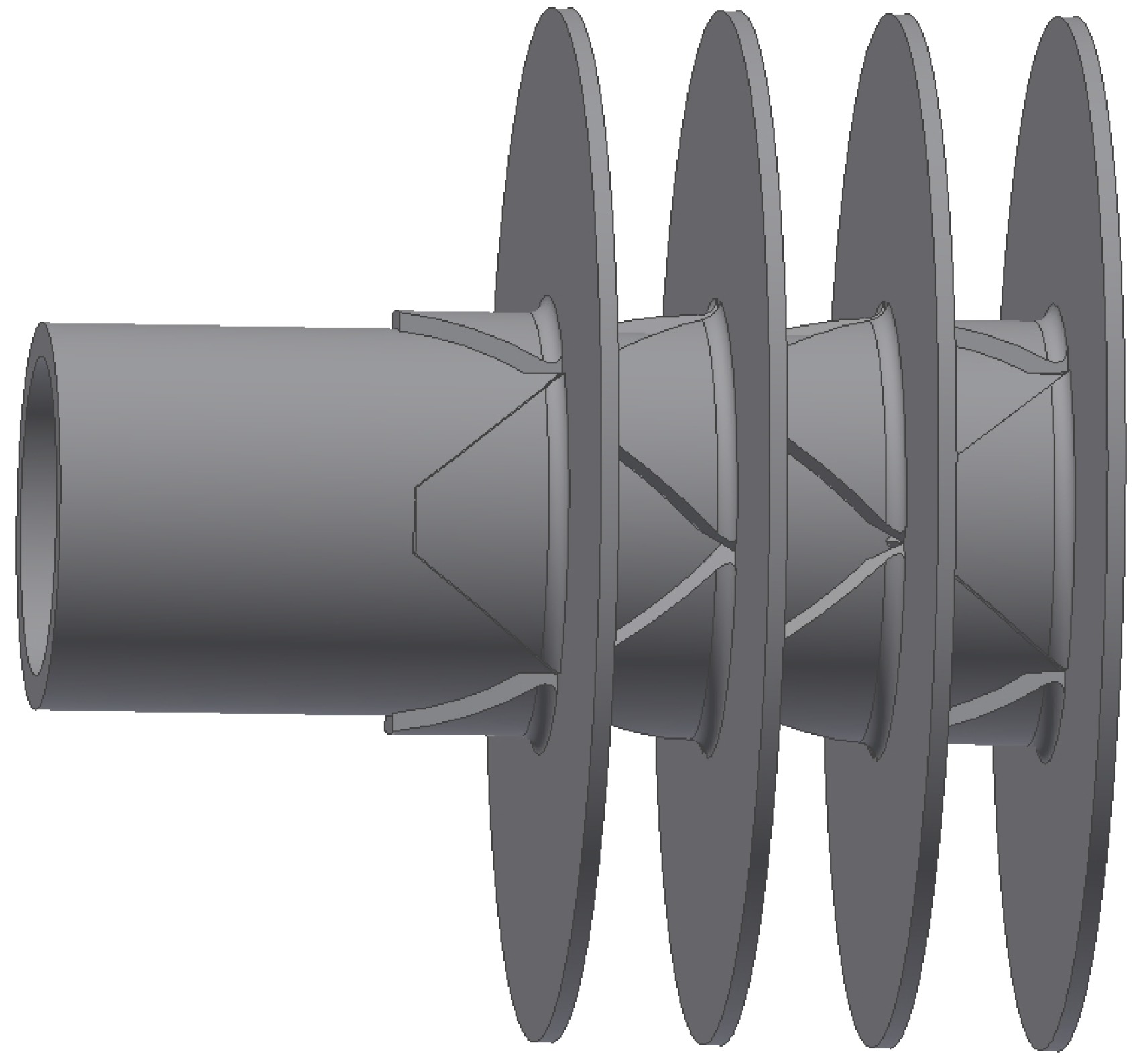
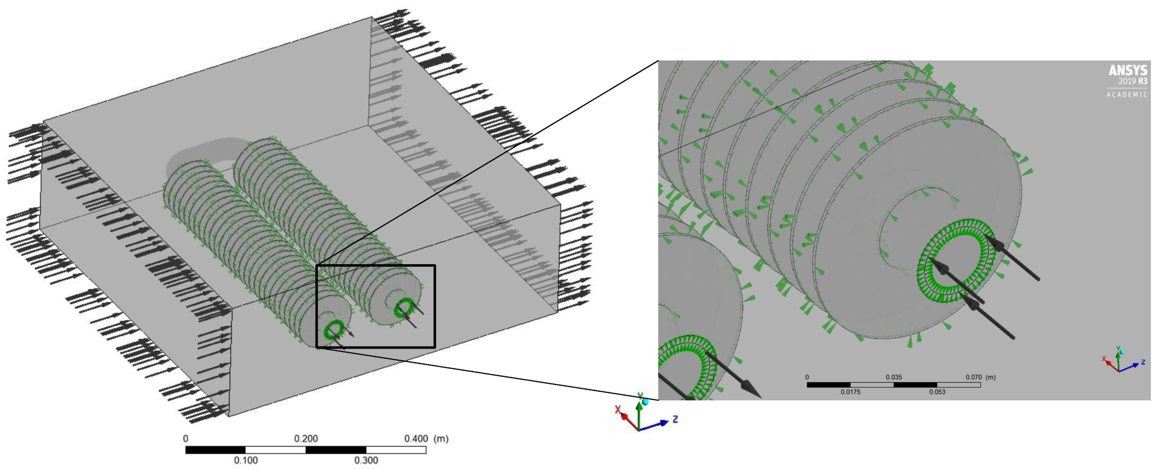
The design and dimensions of the heat exchanger are shown in Figure 3. The tube and the fins were made of carbon steel. Later in the calculations, referring to literature and standard data, the heat conductivity was assumed to be 54 W/mK (according to EN 1993-1-2:2005, for carbon steel). The inner and outer diameters of the tube were $d_i$ = 31 mm and $d_o$ = 37.5 mm respectively; the length of the tube was L = 502.5 mm. The thickness of the fins was $\delta$ = 1.75 mm, the diameter of the fins was D = 100 mm and the space between the fins was $l_f$ = 14.65 mm.

In case of finned tube heat exchangers, several heat transfer surfaces must be defined. Different dimensionless numbers depend on the ratios of these surfaces that are summarized in

Table 1. Different heat transfer areas.

Specific	Sign	Value
inner surface of the tubes	$A_i$	115,193.1 mm${}^2$
surface of 1 bare tube without fins	$A_{t0}$	59,199.38 mm${}^2$
surface of bare tubes without fins	$A_o$	118,398.8 mm${}^2$
surface of the fins	$A_f$	755,945.1 mm${}^2$
total heat transfer area (tubes + fins)	A	913,993.8 mm${}^2$

.

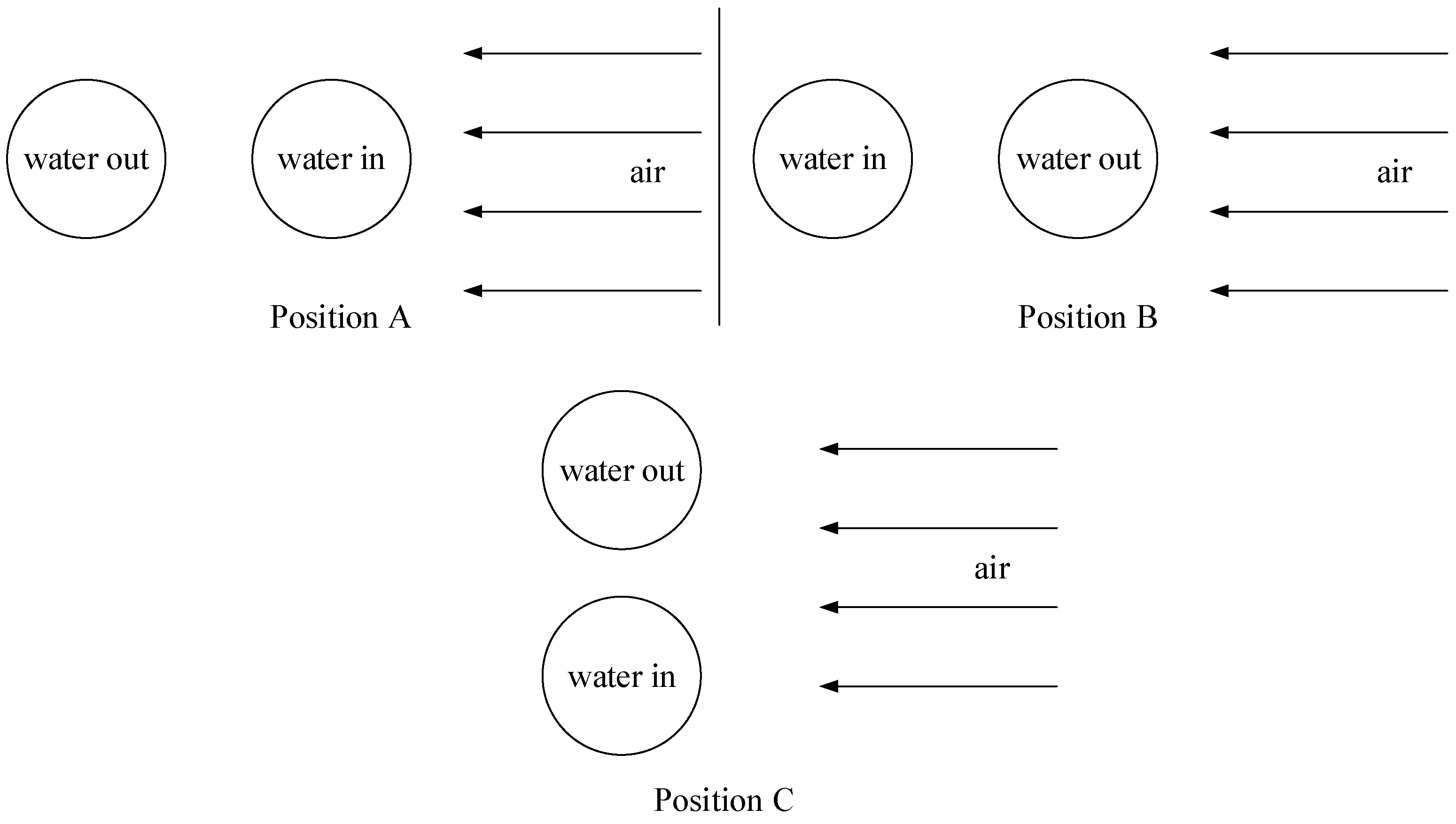
The heat exchanger was placed in three different orientations relative to the air flow, which are shown in Figure 4. Because the air flows perpendicularly to the water in all positions, the cases have been distinguished on the basis of the resulting temperature difference. This difference will be the highest in case of position A and the lowest in case of position B.

2.2. Measurements

As presented in the abstract, the heat exchanger was investigated in three different positions. The volume flow rate of the hot fluid was changed between 100 and 450 L/h (which means fluid velocities of 0.037 m/s and 0.166 m/s respectively), while the velocity of air was changed between 3.3 and 10 m/s. The volume of the tank was large enough not to affect the measurements. In all cases, steady state was expected before the measurements begun. As a result, the smallest possible change in temperature was observed during the study period. The uncertainty in the calculations was based on the standard deviation, and its formula is

$$s=\sqrt{\frac{1}{N-1}\sum _{i=1}^N{\left(T_i-\overline{T}\right)}^2},$$

(1)

where $T_1,T_2,\cdots ,T_N$ are the measured values, $\overline{T}$ is the mean value of those measurements and N is the number of investigated datums. The calculation procedure was as follows: from the measured data (temperatures, volume flow rate), the surface of the heat exchanger and the specific heat at the medium temperature, the amount of heat performance can be determined by the following equation.

$${\dot{Q}}_w={\dot{m}}_w·c_{p,w}·\left(T_{w,in}-T_{w,out}\right)$$

(2)

where $T_{w,in}$ and $T_{w,out}$ are the measured inlet and outlet temperatures of the hot water, ${\dot{m}}_w$ is the mass flow rate and $c_{p,w}$ is the average specific heat of the water, which is the arithmetic mean of the inlet and outlet temperatures. The ${\dot{m}}_w$ can be calculated from the volume flow rate and the density. These material properties, supplemented by viscosity and thermal conductivity, vary with temperature and pressure. During the measurements, the pressure did not change; its value was 1 bar${}_{\mathrm{g}}$ overpressure, so the material properties only depend on the temperature, as is shown in Equation (3).

$$a=a_5·T^5+a_4·T^4+a_3·T^3+a_2·T^2+a_1·T+a_0,$$

(3)

where values of a are constants for water are in

Table 2. Coefficients for properties of water.

	${\mathit{a}}_5$	${\mathit{a}}_4$	${\mathit{a}}_3$	${\mathit{a}}_2$	${\mathit{a}}_1$	${\mathit{a}}_0$
$\rho$	$1.087\times {10}^{-10}$	$-8.826\times {10}^{-8}$	$2.665\times {10}^{-5}$	$-6.009\times {10}^{-3}$	$-2.006\times {10}^{-2}$	1002
$\eta$	$-2.455\times {10}^{-13}$	$8.560\times {10}^{-11}$	$-1.248\times {10}^{-8}$	$1.018\times {10}^{-6}$	$-5.265\times {10}^{-5}$	$1.7331\times {10}^{-3}$
$\lambda$	$-3.590\times {10}^{-13}$	$2.210\times {10}^{-10}$	$-3.407\times {10}^{-8}$	$-5.228\times {10}^{-6}$	$1.803\times {10}^{-3}$	$0.5682$
$c_p$	$-9.672\times {10}^{-10}$	$6.313\times {10}^{-7}$	$-1.1688\times {10}^{-4}$	$1.802\times {10}^{-2}$	$-0.9491$	4195

.

Similarly to the water, the material properties of the air also change in the function of temperature and pressure. However in the wind tunnel, the pressure is ambient (0 bar${}_{\mathrm{g}}$), so the relationships are the following:

$$b=b_5·T^5+b_4·T^4+b_3·T^3+b_2·T^2+b_1·T+b_0,$$

(4)

where the b constants for air are

The material properties calculated by Equations (3) and (4) with coefficients in Table 2 and

Table 3. Coefficients for properties of air.

	${\mathit{b}}_5$	${\mathit{b}}_4$	${\mathit{b}}_3$	${\mathit{b}}_2$	${\mathit{b}}_1$	${\mathit{b}}_0$
$\rho$	$-7.6923\times {10}^{-12}$	$2.028\times {10}^{-9}$	$-2.1993\times {10}^{-7}$	$2.2697\times {10}^{-5}$	$-0.0048$	$1.292$
$\eta$	$-1.60\times {10}^{-17}$	$1.0927\times {10}^{-15}$	$2.9502\times {10}^{-13}$	$-6.561\times {10}^{-11}$	$4.9316\times {10}^{-8}$	$1.7291\times {10}^{-5}$
$\lambda$	$-2.0769\times {10}^{-11}$	$4.8132\times {10}^{-9}$	$-3.802\times {10}^{-7}$	$1.1869\times {10}^{-5}$	$-4.7048\times {10}^{-5}$	$0.0237$
$c_p$	$-6.4103\times {10}^{-9}$	$1.6026\times {10}^{-6}$	$-1.2908\times {10}^{-4}$	$0.0035$	$0.0092$	$1005.9$

have the following dimensions,

• $\rho$ density is kg/m${}^3$;
• $\eta$ dynamic viscosity is Pa·s;
• $\lambda$ thermal conductivity is W/(mK);
• $c_p$ specific heat (for constant pressure) is J/(kgK).

Equations (3) and (4) were prepared by the authors based on UniSim Design (Honeywell International Inc., Charlotte, NC, USA, 2020) process flow simulator data, where the unit of the temperature is ${}^{\circ }$C.

In a fully developed steady state condition, it can be assumed that the heat performance given off by the water is absorbed by the air.

$${\dot{Q}}_w={\dot{m}}_a·c_{p,a}·\left(T_{a,in}-T_{a,out}\right),$$

(5)

where the outlet temperature of air ($T_{a,out}$) can be calculated. The outlet temperature can be neglected since a relatively large amount of air flows in the wind tunnel.

The relationship between the heat performance of heat exchangers is known:

$${\dot{Q}}_w=k·A·\Delta T_{LOG},$$

(6)

where A is the total heat transfer area (from Table 1); the $\Delta T_{LOG}$ is the logarithmic mean temperature difference (LMTD) of the inlet and outlet temperatures. The only unknown value is the overall heat transfer coefficient, which was derived from Equations (2) and (6):

$$k=\frac{{\dot{m}}_w·c_{p,w}·\left(T_{w,in}-T_{w,out}\right)}{A·\Delta T_{LOG}}.$$

(7)

The aim of this present study is to compare the heat transfer coefficients from experimental, numerical and empirical relationships, and to develop a generally applicable relationship for this type of finned tube heat exchanger.

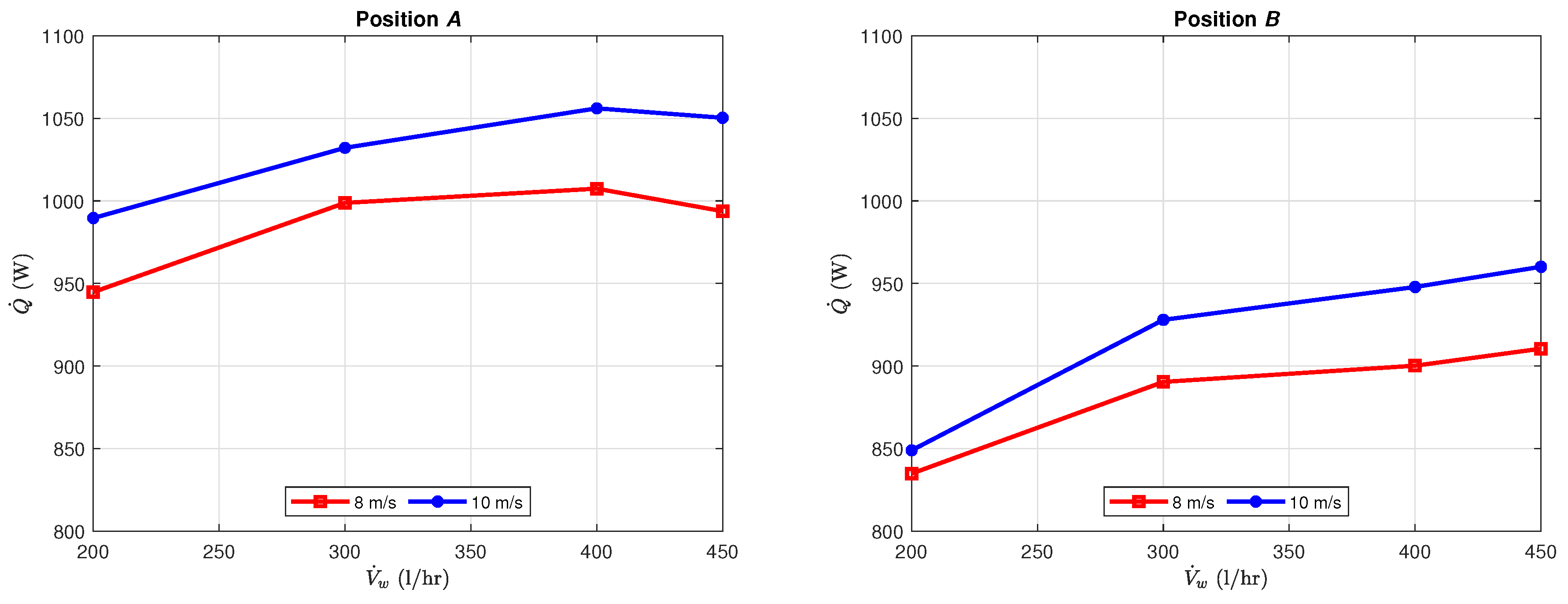
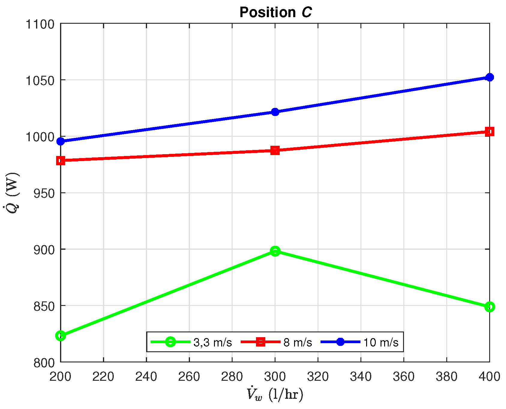
Figure 5 shows the results of the measurements. In every case, the measurement took two minutes after the steady state with a 5 Hz sample rate in positions A, B and C, as shown in Figure 4. The graphs show that in positions A, when the higher temperature water comes into contact with the air first, the heat performance will be a higher than in position B. This is explained by the fact that at this position the temperature difference (LMTD), in other words the driving force, will be larger. The heat performances experienced in the cross-current case (position C) are roughly the same as in the quasi-counter current case (position A).

Table 4. Results of measurement in position A.

	ID1	ID2	ID3	ID4	ID5	ID6	ID7	ID8
${\dot{V}}_{water}$	200	200	300	300	400	400	450	450
$v_{air}$	8	10	8	10	8	10	8	10
$T_{in}$	57.19	57.12	57.15	57.08	57.09	57.05	57.07	57.04
$s_{T_{in}}$	0.023	0.026	0.022	0.023	0.025	0.027	0.024	0.019
$T_{out}$	53.07	52.81	54.24	54.08	54.89	54.75	55.14	55.01
$s_{T_{out}}$	0.034	0.026	0.021	0.018	0.024	0.019	0.022	0.018
$\Delta T$	4.12	4.32	2.91	3.00	2.20	2.30	1.93	2.04
$s_{\Delta T}$	0.032	0.017	0.0120	0.020	0.024	0.020	0.027	0.013

,

Table 5. Results of measurement in position B.

	ID11	ID12	ID13	ID14	ID15	ID16	ID17	ID18
${\dot{V}}_{water}$	200	200	300	300	400	400	450	450
$v_{air}$	8	10	8	10	8	10	8	10
$T_{in}$	57.01	56.83	56.69	56.74	56.86	56.93	57.09	57.17
$s_{T_{in}}$	0.028	0.106	0.028	0.019	0.034	0.032	0.047	0.025
$T_{out}$	53.37	53.13	54.10	54.04	54.89	54.86	55.33	55.31
$s_{T_{out}}$	0.106	0.031	0.031	0.017	0.029	0.031	0.045	0.026
$\Delta T$	3.64	3.70	2.59	2.70	1.96	2.07	1.77	1.86
$s_{\Delta T}$	0.118	0.092	0.016	0.012	0.018	0.019	0.043	0.022

and

Table 6. Results of measurement in position C.

	ID21	ID22	ID23	ID24	ID25	ID26	ID27	ID28	ID29	ID30
${\dot{V}}_{water}$	200	200	200	300	300	300	400	400	400	100
$v_{air}$	3.3	8	10	3.3	8	10	3.3	8	10	10
$T_{in}$	57.13	57.32	57.35	56.98	56.98	56.97	57.04	57.13	57.12	56.81
$s_{T_{in}}$	0.047	0.035	0.042	0.059	0.026	0.033	0.027	0.026	0.021	0.050
$T_{out}$	53.54	53.05	53.01	54.37	54.11	53.00	55.18	54.93	54.82	50.81
$s_{T_{out}}$	0.040	0.029	0.054	0.277	0.025	0.039	0.038	0.024	0.024	0.327
$\Delta T$	3.59	4.27	4.34	2.61	2.87	2.97	1.85	2.19	2.30	6.00
$s_{\Delta T}$	0.070	0.053	0.034	0.332	0.015	0.049	0.028	0.020	0.014	0.303

show the measured values and the standard deviation: $s_{T_{in}}$ for the inlet temperature, $s_{T_{out}}$ for the outlet temperature and $s_{\Delta T}$ for the temperature difference:

The measured values ($T_{in}$, $T_{out}$) in Table 4, Table 5 and Table 6 are the average temperatures during the measurements in stationary state, and the standard deviations calculated with Equation (1).

According to the measured values it can be seen that the biggest temperature difference was reached in the case of position A, and the heat performance of position C is relatively close to it.

3. Numerical Simulation

3.1. Computational Domains

The results of the measurement at position B were validated by performing numerical simulations. The three dimensional geometry model was imported to ANSYS-CFX (ANSYS, Inc., Canonsburg, USA). Five different computational domains were considered: tubes, fins on the first row, fins on the second row, inside medium and the outside volume. Heat conduction was considered in the first three of the domains, while forced convection in the other two cases. The material of the tubes and fins was ferritic steel; the inside medium was water; and the outside volume was air.

As mentioned, the fins and the tube were modeled as solid domains, and the material properties were set up for steel. The air and the water were modeled as fluid domains, and the SST (shear stress transport) turbulence model was set up for both materials. In order to calculate heat transfer through the different computational domains, interfaces had to be set up. These interfaces are indicated by green arrows in Figure 6.

3.2. Boundary Conditions

The results of the measurements were used as the basis for setting the boundary conditions. In the models there are two inlet surfaces in all cases: one for the air and another for the water. It can be assumed that a parallel flow develops in a wind tunnel, so it is sufficient to specify the velocity, the temperature and the intensity value for the air inlet. An additional computational domain was added to the air inlet and outlet where the boundary conditions were applied.

Depending on the Re number, a turbulent case occurs in the flow of water in the tube, but there will certainly not be a backflow; therefore, similar characteristics were used for the water inlet. For both air side and water side, the inlet boundary conditions are shown in Table 4, Table 5 and Table 6.

The sizes of the outlet surfaces were the same as the inlet surfaces, and average static pressure outlet boundary conditions were set up like the outlet boundaries. The zero total pressure boundary condition was applied on both outlets.

In the cases of the wall boundaries, interfaces had to be used between the connections. The 56 fins and the tube thus resulted in a total of 226 interfaces using heat flux setting. Prism-layer insertions were used in every interface. Mesh independence test was performed.

Studies were performed with the presented settings, but with k-$\epsilon$ turbulence model. Based on that, the heat performances were even lower, so there are even higher differences (average 45%) between the measurements and the simulations.

3.3. Results

Table 7. Comparison of measurements and numerical simulations.

ID	Measurements				Simulation	Differences
	${\dot{\mathit{V}}}_{\mathit{w}}$	${\mathit{v}}_{\mathit{a}}$	${\mathit{T}}_{\mathit{w},\mathit{in}}$	${\dot{\mathit{Q}}}_{\mathit{m}}$	${\dot{\mathit{Q}}}_{\mathit{CFD}}$	$\mathbf{\Delta }\dot{\mathit{Q}}$	%
ID1	200	8	57.19	944.73	756.18	188.55	19.96%
ID2	200	10	57.12	989.57	804.09	185.48	18.74%
ID3	300	8	57.15	998.79	777.85	220.95	22.12%
ID4	300	10	57.08	1032.14	833.53	198.61	19.24%
ID5	400	8	57.09	1007.40	793.65	213.75	21.22%
ID6	400	10	57.05	1056.05	857.35	198.70	18.82%
ID7	450	8	57.07	993.73	801.57	192.16	19.34%
ID8	450	10	57.04	1050.32	868.58	181.74	17.30%

shows the results and the differences of the measurements and the numerical simulations.

It can be seen from the obtained results that the heat performances of the CFD analysis are consistently 17–22 % lower than the heat performances of the measurements. This error may be due to the fact that the fins on the measured heat exchanger were not planar, but had four protrusions on them. The fins were made from planar plates with two perpendicular cuts, which is shown in Figure 7.

The simplification assumed that the geometric model would give the same results as the measurement. However, it can be seen that these four small protrusions caused a small heat transfer surface increment, and moreover, had a turbulence-increasing effect.

From the obtained results it can be stated that the geometry of the examined fins increases the heat transfer coefficient by 19.58% on average, and thus the heat performance of the structure was different to the planar shape.

4. Empirical Calculations

4.1. VDI Theorem

The usage of the fins as extended surfaces will create a higher heat transfer area and also a lower heat transfer coefficient. These fins represent a resistance in the flow, which will cause a higher velocity and degree of turbulence, which would mean a higher value of heat transfer coefficient. However the heat is not only transferred from the water to the air by convection, but also with conduction along the fins. As a result, the surface temperature of the fins has a lower value, so the higher theoretical heat transfer coefficient does not affect a higher transferred heat, because of the lower temperature difference. To take this into account, an efficiency value and a modified heat transfer coefficient must be calculated as functions of the geometry of the fins. The following relationships are available in the VDI-Heat atlas (abbrevation of the german Verein Deutscher Ingenieure) [18]. This modified heat transfer coefficient is

$${\alpha }_v={\alpha }_m\left[1-\left(1-{\eta }_f\right)\frac{A_f}{A}\right],$$

(8)

where ${\alpha }_m$ is the theoretical heat transfer coefficient without the fins (as a smooth tube), ${\eta }_f$ is the efficiency, $A_f$ is the heat transfer area of the single fins and A is the total heat transfer area. The calculation of the theoretical heat transfer coefficient is analogous to the calculations of any other types of convections: with experimental Nu-number correlation. In the case of a finned tube heat exchanger, two different cases can be extinguished: inline (9) and staggered (10) layout:

$$Nu=0.22·R{e}^{0.6}·{\left(\frac{A}{A_{t0}}\right)}^{-0.15}·P{r}^{0.33}\mathrm{and}$$

(9)

$$Nu=0.38·R{e}^{0.6}·{\left(\frac{A}{A_{t0}}\right)}^{-0.15}·P{r}^{0.33}.$$

(10)

The value of the efficiency highly depends on the shape of the fins. This study investigated the circular shape, so the correlation related to this type. First of all, a geometric parameter must be calculated, which depends on the diameter of the tube ($d_o$) and the diameter of the fin (D):

$$\phi =\left(\frac{D}{d_o}-1\right)·\left[1+0.35·ln\left(\frac{D}{d_o}\right)\right].$$

(11)

The following X parameter is used to express the disadvantageous effect of the fins on the heat transfer coefficient, which contains the heat transfer coefficient over the smooth tube; the heat conductivity and thickness of the fins; and the previously calculated $\phi$ parameter.

$$X=\phi ·\frac{d_o}{2}\sqrt{\frac{2·{\alpha }_m}{{\lambda }_f·\delta }}.$$

(12)

The efficiency can be calculated with Equation (13)

$${\eta }_f=\frac{tanhX}{X}.$$

(13)

and Figure 8 shows its graphic definition.

According Equation (13) and Figure 8, the value of the overall heat transfer coefficient for the finned tube heat exchanger is

$$\frac{1}{k}=\frac{1}{{\alpha }_v}+\frac{A}{A_i}\left(\frac{1}{{\alpha }_i}+\frac{d_o-d_i}{2·{\lambda }_t}\right).$$

(14)

Table 8. Comparison of measurements and analytical calculations.

ID	Measurements		Calculations		Differences
	$\dot{\mathit{Q}}$	$\mathit{k}$	$\dot{\mathit{Q}}$	$\mathit{k}$	$\Delta \dot{\mathit{Q}}$	%
ID1	944.73	34.71	366.69	13.48	578.04	61.19
ID2	989.57	36.56	368.49	13.61	621.08	62.76
ID3	998.79	35.98	417.13	15.03	581.66	58.24
ID4	1032.14	37.32	441.28	15.96	590.86	57.25
ID5	1007.4	35.92	461.03	16.44	546.37	54.24
ID6	1056.05	37.78	491.01	17.56	565.04	53.51
ID7	993.73	35.31	478.41	16.99	515.32	51.86
ID8	1050.32	37.42	510.91	18.20	539.41	51.36

summarizes the results of the measurements and the analytical calculations.

It is clearly seen from the table that the heat transfer coefficients calculated with the method chosen from the literature are significantly lower than the measured values.

4.2. Schmidt theorem

There is another empirical calculation method to calculate the heat transfer coefficient and the heat performance. According to Schmidt [19], the easiest way to calculate the dimensionless numbers is to calculate them with the hydraulic diameter of the device. This effective diameter depends on the outer diameter of the tube and the quotient of the area of the finned tube and the area of the bare tube:

$$d_F=d_o·\frac{A}{A_0}$$

(15)

The necessary dimensionless numbers, the Re and Nu numbers, are calculated with this hydraulic length.

$$R{e}_F=\frac{v·d_F·\rho }{\eta }$$

(16)

$$N{u}_F=\frac{{\alpha }_F·d_F}{\lambda }$$

(17)

The empirical Nu number definition is

$$N{u}_F=C_F·R{e}_F^{0.625}·P{r}^{1/3},$$

(18)

where the $C_F$ constant is 0.30 for inline and 0.45 for staggered layout. Applying Equations (15)–(18) to the investigated cases,

Table 9. Comparison of measurements and analytical calculations.

ID	Measurements		Calculations		Differences
	$\dot{\mathit{Q}}$	$\mathit{k}$	$\dot{\mathit{Q}}$	$\mathit{k}$	$\Delta \dot{\mathit{Q}}$	%
ID1	944.73	34.71	925.25	33.99	19.49	2.06
ID2	989.57	36.56	1031.80	38.12	−42.23	−4.27
ID3	998.79	35.98	989.19	35.63	9.6	0.96
ID4	1032.14	37.32	1111.83	40.21	−79.69	−7.72
ID5	1007.4	35.92	1025.59	36.57	−18.19	−1.81
ID6	1056.05	37.78	1157.52	41.41	−101.47	−9.61
ID7	993.73	35.31	1039.03	36.91	−45.3	−4.56
ID8	1050.32	37.42	1174.57	41.84	−124.25	−11.83
ID11	834.81	33.16	855.04	33.96	−20.23	−2.42
ID12	848.90	33.97	951.69	38.09	−102.79	−12.11
ID13	890.35	35.08	903.28	35.59	−12.93	−1.45
ID14	927.94	36.57	1018.97	40.15	−91.04	−9.81
ID15	900.17	34.85	943.69	36.53	−43.52	−4.83
ID16	947.84	36.67	1069.29	41.36	−121.45	−12.81
ID17	910.47	34.83	963.95	36.88	−53.48	−5.87
ID18	960.09	36.69	1093.96	41.81	−133.88	−13.94

shows the results for position A and position B, the inline layouts.

The results show that with this theorem it is possible to determine the expected heat performances more accurately than with the VDI correlations. From the data shown in Table 9, it can be seen that with this method the calculated performances are overestimated the measured values, and these differences are between +2.06 and −13.94%. Applying the least squares regression method to the measured data, the C constant and the exponent of Re number were searched in the form of Equation (18).

The proposed equation for this case should be

$$Nu=29.5956·R{e}_F^{0.2371}·P{r}^{1/3},$$

(19)

and

Table 10. Comparison of measurements and analytical calculations with the modified correlation.

ID	Measurements		Calculations		Differences
	$\dot{\mathit{Q}}$	$\mathit{k}$	$\dot{\mathit{Q}}$	$\mathit{k}$	$\Delta \dot{\mathit{Q}}$	%
ID1	944.73	34.71	905.16	33.26	−39.57	−4.19
ID2	989.57	36.56	940.68	34.76	−48.89	−4.94
ID3	998.79	35.98	966.71	34.83	−32.08	−3.21
ID4	1032.14	37.32	1008.65	36.47	−23.49	−2.28
ID5	1007.40	35.92	1001.69	35.72	−5.71	−0.57
ID6	1056.05	37.78	1047.15	37.46	−8.90	−0.84
ID7	993.73	35.31	1014.59	36.05	20.86	2.10
ID8	1050.32	37.42	1061.50	37.81	11.18	1.06
ID11	834.81	33.16	837.27	33.26	2.45	0.29
ID12	848.90	33.97	868.48	34.76	19.58	2.31
ID13	890.35	35.08	883.96	34.83	−6.39	−0.72
ID14	927.94	36.57	925.58	36.47	−2.36	−0.25
ID15	900.17	34.85	922.79	35.72	22.62	2.51
ID16	947.84	36.67	968.37	37.46	20.53	2.1
ID17	910.47	34.83	942.24	36.05	31.77	3.49
ID18	960.09	36.69	989.53	37.81	29.44	3.07

shows the values calculated with this equation.

It is seen from Table 10 that the calculated heat transfer coefficient (k) was the same in both positions. This can be explained by the fact that for these calculated values with the same empirical correlation (Equation (19)), the difference in heat performance is due to the logarithmic mean temperature difference.

The heat performances and heat transfer coefficients for position C calculated with the original Schmidt correlation (Equation (18)) are shown in

Table 11. Comparison of measurements and analytical calculations.

ID	Measurements		Calculations		Differences
	$\dot{\mathit{Q}}$	$\mathit{k}$	$\dot{\mathit{Q}}$	$\mathit{k}$	$\Delta \dot{\mathit{Q}}$	%
ID21	823.24	30.74	563.08	21.03	260.16	31.60
ID22	978.44	36.74	905.06	33.99	73.38	7.50
ID23	995.44	37.39	1015.00	38.13	−19.56	−1.97
ID24	898.20	33.14	586.56	21.64	311.64	34.70
ID25	987.34	36.59	961.12	35.62	26.22	2.66
ID26	1021.49	37.94	1081.97	40.19	−60.48	−5.92
ID27	848.86	30.86	604.88	21.99	234.98	28.74
ID28	1004.11	36.60	1003.21	36.57	0.90	0.09
ID29	1052.26	38.43	1133.53	41.40	−81.27	−7.72

.

The differences in Table 11 show that the Schmidt relation cannot be applied to the real cross current either; therefore, the least squares method has been applied to this case as well. The result of this method is given in Equation (20) and the calculated heat performances with this is shown in

Table 12. Comparison of measurements and analytical calculations with the modified correlation.

ID	Measurements		Calculations		Differences
	$\dot{\mathit{Q}}$	$\mathit{k}$	$\dot{\mathit{Q}}$	$\mathit{k}$	$\Delta \dot{\mathit{Q}}$	%
ID21	823.24	30.74	814.48	30.42	−8.76	−1.06
ID22	978.44	36.74	932.65	35.02	−45.79	−4.68
ID23	995.44	37.39	965.58	36.27	−29.85	−3.00
ID24	898.20	33.14	859.61	31.72	−38.59	−4.30
ID25	987.34	36.59	991.87	36.76	4.53	0.46
ID26	1021.49	37.94	1026.58	38.13	5.09	0.50
ID27	848.86	30.86	893.09	32.46	44.23	5.21
ID28	1004.11	36.60	1036.19	37.77	32.08	3.19
ID29	1052.26	38.43	1073.85	39.22	21.59	2.05

.

$$Nu=55.4028·R{e}_F^{0.1897}·P{r}^{1/3},$$

(20)

Table 12 shows that the heat performances calculated with the developed Nu correlation become much more accurate than with the original correlation.

5. Conclusions

In this study, the heat transfer performances of circular finned tube banks subject to different settlements were demonstrated.

Based on the foregoing discussion, the following conclusions are made:

(1)

Even in the case of relatively small geometric sizes, the flow directions are obviously important for the heat performance. In the case of the finned tube shown in the experiments the countercurrent and cross-current connections are recommended.

(2)

The results of the numerical simulations correlate quite well with the experimental results. However it has been proven that the irregularities and protrusions on the experimental equipment are significant to the final heat performance. Those effected the increased value of performance by an average of 19.58%, which could result in significant material savings in an optimization task.

(3)

The calculation method in VDI Heat Atlas can be used in many ways and is close to reality if the heat transfer coefficient inside the tube is orders of magnitude higher than the heat transfer coefficient on the air side. In this present study, a transient flow developed inside the tube, which causes only an order of magnitude larger coefficient than the air side, so it has a greater effect on the overall heat transfer coefficient.

(4)

New Nu number relationships are proposed for U-shaped finned exchangers. Those cause differences of −4.94 and +5.21 percent in the examined cases.

References

1. Bavasarajappa, S.; Manavendra, G.; Prakash, S.B. A review on performance study of finned tube heat exchanger. J. Phys. Conf. Ser. 2020, 1473, 012030. [Google Scholar] [CrossRef]
2. Bhuiyan, A.A.; Islam, A.K.M.S. Thermal and hydraulic performance of finned-tube heat exchangers under different flow ranges: A review on modeling and experiment. Int. J. Heat Mass Transf. 2016, 101, 38–59. [Google Scholar] [CrossRef]
3. Pongsoi, P.; Pikulkajorn, S.; Wongwises, S. Heat transfer and flow characteristics of spiral fin-and-tube heat exchangers: A review. Int. J. Heat Mass Transf. 2014, 79, 417–431. [Google Scholar] [CrossRef]
4. Unger, S.; Beyer, M.; Szalinski, L.; Hampel, U. Thermal and flow performance of tilted oval tubes with novel fin designs. Int. J. Heat Mass Transf. 2020, 153, 119621. [Google Scholar] [CrossRef]
5. Chai, L.; Tassou, S.A. A review of airside heat transfer augmentation with vortex generators on heat transfer surface. Energies 2018, 11, 2737. [Google Scholar] [CrossRef] [Green Version]
6. Sheikholeslami, M.; Gorji-Bandpy, M.; Ganji, D.D. Fluid flow and heat transfer in an air-to-water double-pipe heat exchanger. EPJ Plus 2015, 130, 1–12. [Google Scholar] [CrossRef]
7. Unger, S.; Beyer, M.; Arlit, M.; Stasch, P.; Hampel, U. An experimental investigation on the air-side heat transfer and flow resistance of finned short oval tubes at different tube tilt angles. Int. J. Heat Mass Transf. 2019, 140, 225–237. [Google Scholar] [CrossRef]
8. Peng, P. Research on Structural Optimization of Spiral Array Heat Exchanger Based on Exhaust Heat Recovery. IOP Conf. Ser. Mater. Sci. Eng. 2020, 782, 032025. [Google Scholar] [CrossRef]
9. Syuhada, A.; Afandi, D.; Sofyan, S.E. Convective heat transfer study on the spiral finned tube heat exchanger under various fin pitch arrangements. IOP Conf. Ser. Earth Environ. Sci. 2020, 463, 012024. [Google Scholar] [CrossRef] [Green Version]
10. Wang, C.C.; Fu, W.L.; Chang, C.T. Heat Transfer and Friction Characteristics of Typical Wavy Fin-and-Tube Heat Exchangers. Exp. Therm. Fluid Sci. 1997, 14, 174–186. [Google Scholar] [CrossRef]
11. Bhale, P.; Kaushik, M.; Liaw, J.S.; Wang, C.C. Airside performance of H-type finned tube banks with surface modifications. Energies 2019, 12, 584. [Google Scholar] [CrossRef] [Green Version]
12. Moorty, P.; Oumer, A.N.; Ishak, M. Experimental Investigation on Effect of Fin Shape on the Thermal-Hydraulic Performance of Compact Fin-and-Tube Heat Exchangers. IOP Conf. Ser. Mater. Sci. Eng. 2018, 318, 12–70. [Google Scholar] [CrossRef]
13. Yao, J. A Review of Industrial Heat Exchange Optimization. IOP Conf. Ser. Earth Environ. Sci. 2018, 108, 042036. [Google Scholar] [CrossRef]
14. Taler, D.; Taler, J.; Trojan, M. Thermal calculations of plate–fin–and-tube heat exchangers with different heat transfer coefficients on each tube row. Energies 2020, 203, 117806. [Google Scholar] [CrossRef]
15. Petrik, M.; Szepesi, G.; Jármai, K. CFD analysis and heat transfer characteristics of finned tube heat exchangers. Pollack Period. 2019, 14, 165–176. [Google Scholar] [CrossRef]
16. Nemati, H.; Moghomi, M. Numerical Study of Flow Over Annular-Finned Tube Heat Exchangers by Different Turbulent Models. CFD Lett. 2014, 6, 101–112. [Google Scholar]
17. Mon, M.S.; Gross, U. Numerical study of fin-spacing effects in annular-finned tube heat exchangers. Int. J. Heat Mass Transf. 2004, 47, 1953–1964. [Google Scholar] [CrossRef]
18. VDI Heat Atlas, VDI-Gesellschaft Verfahrenstechnik und Chemieingenieurwesen (VDI-GVC); Springer: Düsseldorf, Germany, 2010. [CrossRef]
19. Schmidt, T.E. Der Wärmeübergang an Rippenrohre und die Berechnung von Rohrbündel-Wärmeaustauscher. Kältetechnik 1963, 15, 98–102. [Google Scholar] [CrossRef]
Figure 1. Investigated heat exchanger.
Processes 08 00773 g001
Figure 2. Experimental setup.
Processes 08 00773 g002
Figure 3. Dimensions of the investigated heat exchanger.
Processes 08 00773 g003
Figure 4. Orientation of heat exchanger relative to the air flow.
Processes 08 00773 g004
Figure 5. Results of the measurements.
Processes 08 00773 g005aProcesses 08 00773 g005b
Figure 6. The investigated geometry.
Processes 08 00773 g006
Figure 7. The protrusions on the tubes.
Processes 08 00773 g007
Figure 8. Graphic definition of the efficiency.
Processes 08 00773 g008