Article

Research on State Recognition and Failure Prediction of Axial Piston Pump Based on Performance Degradation Data

1
Hebei Provincial Key Laboratory of Heavy Machinery Fluid Power Transmission and Control, Yanshan University, Qinhuangdao 066004, China
2
The State Key Laboratory of Fluid Power and Mechatronic Systems, Zhejiang University, Hangzhou 310027, China
3
Key Laboratory of Advanced Forging and Stamping Technology and Science, Yanshan University, Qinhuangdao 066004, China
4
Hebei Key Laboratory of Special Delivery Equipment, Yanshan University, Qinhuangdao 066004, China
*
Author to whom correspondence should be addressed.
Processes 2020, 8(5), 609; https://doi.org/10.3390/pr8050609
Submission received: 25 March 2020 / Revised: 15 May 2020 / Accepted: 15 May 2020 / Published: 20 May 2020

Abstract

:
Degradation state recognition and failure prediction are the key steps of prognostic and health management (PHM), which directly affect the reliability of the equipment and the selection of preventive maintenance strategy. Given the problem that the distinction between feature vectors is not obvious and the accuracy of fault prediction is low, a method based on multi-class Gaussian process classification and Gaussian process regression (GPR) is studied by the vibration signal and flow signal in six degraded states of the axial piston pump. For degradation state recognition, the variational mode decomposition (VMD) was used to decompose the vibration signal, and obtaining intrinsic mode function (IMF) components with rich information. Subsequently, multi-scale permutation entropy (MPE) was employed to select feature vectors of IMF components in different states. In order to reduce feature dimensions and improve recognition performance, ReliefF was used to select feature vectors with high weight, then a method based on multi-class Gaussian process classification was established by using these feature vectors to realize the research on the degradation state recognition. The test results demonstrate that the method can effectively identify the degradation state. Its recognition rate reaches 98.9%. Besides, for failure prediction, through the analysis of the wear process and wear mechanism of the valve plate, the curve fitting between the flow and the wear amount was performed by GPR to realize the failure prediction of the axial piston pump. Depending on the evaluation index, the GPR obtained a better failure prediction effect. The results will assist in the realization of predictive maintenance, and which also has significant practical value in project items.

1. Introduction

As the most commonly used hydraulic pump, the axial piston pump directly affects the stability of the entire hydraulic system. Therefore, it is extremely important to study state identification and failure prediction [1,2]. The essence of failure prediction and state identification for equipment is to extract the feature vectors that can reflect the degradation state of the equipment. The failure time of the equipment can be predicted according to the change of the feature vectors, and the state identification can be realized by distinguishing the characteristic variables in different states. Due to the compressibility of the hydraulic fluid, the fluid-solid coupling vibration, the hydraulic circuit and the inherent mechanical shock of the pump body during working, the characteristics about strong non-stationary and non-linear are exhibited from signals [3], so the degradation feature vectors extracted in these signals become the key to status recognition and failure prediction. By studying the degradation state identification and fault prediction of axial piston pump, the occurrence of the failure can be predicted as well as prevented, unnecessary and expensive preventive maintenance can be eliminated, the maintenance plan can be optimized, the lead time of spare parts and resources can be reduced, and the cost can be greatly saved [4].
For studies of the state recognition and failure prediction of equipment, the literature [5] proposed a feature extraction method of the gear vibration signals by combining wavelet coefficients and local Gaussian correlation. The multifractal detrended fluctuation analysis (MF-DFA) method was used in literature [6] to select the characteristics for the process of gearbox degradation. The literature [7] proposed a method based on S transform relative spectrum entropy to extract the degraded features and the weighted gray correlation analysis method was used to realize the degraded state recognition of the hydraulic pump, the effectiveness of the method has been verified by analyzing the wear faults of the sliding shoes and the loose slipper. Talking about the literature [8], a fault diagnosis method based on redundant second-generation wavelet packet transform (RSGWPT), neighborhood rough set (NRS) and support vector machine (SVM) was proposed. In the literature [9], the Kernel Principal component analysis (KPCA) method served to obtain the new characteristic variables based wavelet correlation feature scale entropy (WCFSE) that are used as the input for training, to establish a hidden Semi–Markov model (HSMM), which achieving degraded state recognition and failure prediction.
Most of the research methods for state identification and failure prediction of piston pump are based on the methods applicable to rotating machinery. Gao et al. [10] studied the state monitoring method for piston pump based on wavelet packet analysis. Sun et al. [11] combined Local characteristic-scale decomposition (LCD) and composite spectral entropy, then applied it to the degenerative feature extraction of the axial piston pump. Wang et al. [12] evaluated the fusion of vibration signal and pressure signal to extract feature vectors, then used principal component analysis (PCA) and back propagation (BP) neural network to realize the fault diagnosis of loose slipper with pumps. Wu et al. [13] used a Bayesian network to provide a piston pump fault diagnosis method based on multi-feature fusion of evidence theory. Zhang et al. [14] decomposed the vibration signals into a set of intrinsic mode functions (IMFs) through the ensemble empirical mode decomposition (EEMD), selected the first several IMFs to calculate permutation entropy (PE) values as the feature vectors, and then used SVM to classify the fault type as well as fault severity. In the same way, Lu et al. [15] used the EEMD method to decompose pressure signal, selected useful IMFs through correlation coefficient. Principal component analysis (PCA) was then employed to reduce the dimensionality of the original feature vectors. Finally, support vector regression (SVR) is constructed to identify different fault sizes of the aviation pump.
Aiming at the nonlinear dynamic characteristics of degraded signals, there are many methods in the field of failure prediction and state recognition, such as correlation dimension [16], approximate entropy [17,18], sample entropy [19], fuzzy entropy [20], PE [21], all of them have achieved some results. However, each of these methods has its shortcomings. When calculating the correlation dimension of detail component, there are problems of large amount of calculation and long calculation time [22]. Approximate entropy and sample entropy are both quantitative statistical indexes of signal complexity [23]. If there is a small change near the threshold parameter, different results will be caused by the hard threshold criterion, which affecting the statistical stability. The definition of fuzzy entropy is built on the concept of membership function, which is usually difficult and inaccurate [24]. PE only detects the randomness and dynamic mutation of time series on a single scale [25]. Compared with PE, multiscale permutation entropy (MPE) is more robust. MPE is used to measure the complexity and randomness of time series at different scales [26]. During the operation of the axial piston pump, the randomness of vibration signal and dynamic behavior will change due to the different wear degrees of valve plates. Therefore, MPE, as feature vector, is used to measure the random change and the dynamic mutation of vibration signals.
After extracting the degraded features, it is necessary to reduce the dimension of the features, because these features can not be guaranteed to be equally useful in reflecting the degraded state. In addition, the calculation burden will be increased because of too much input variables. Common methods of dimensionality reduction include PCA [27], lasso [28] and KPCA [29]. ReleifF [30,31] finds the features with strong classification ability without losing the original physical meaning, which is beneficial to distinguish the nearest neighbor of the same kind and different kinds. Therefore, ReleifF is introduced to obtain sensitive degraded features in MPE.
For state recognition, the popular classification methods are decision tree [32], k-nearest neighbor (KNN) [33], artificial neural network (ANN) [34], SVM [35], these algorithms have their advantages and disadvantages in sample classification, among which SVM based on kernel function is the most popular because kernel method has incomparable advantages in dealing with high-dimensional and nonlinear problems [36]. In recent years, the Gaussian process classification algorithm based on kernel function has also caught the attention of many researchers. Compared with other kernel function classifiers, the advantage of the Gaussian process classifier is to use a probability model [37], which outputs a probability instead of certain value. The Gaussian classifier is a parameter-free model, because the parameters are automatically obtained in the algorithm solution process [38]. Gaussian process classifier that can only be used to solve the two classification problems directly is similar to the SVM classifier. So how to build multi-class Gaussian process classification based on binary Gaussian process classification is of great significance. For failure prediction, compared with other regression models, the advantage of Gaussian process regression (GPR) [39] is that the model is based on Bayesian framework, and the predicted value is also probabilistic, so the confidence interval can be calculated, and then the prediction can be refitted in a useful region according to this information.
In this paper, experimental research on different wear state of the valve plate for axial piston pump was carried out. Aiming at the state recognition of axial piston pump, this paper used in variational mode decomposition (VMD) method to select the best IMF to remove the influence of noise by kurtosis index, then the suitable feature vectors were obtained by MPE and ReliefF. Finally, the multi-class Gaussian process classification was used to realize state identification. Aiming at the failure prediction for axial piston pump, the VMD was utilized to process the experimental data of the flow signal, and the average flow of selected best IMF was obtained. Finally, the GPR method was utilized to fit the prediction curve of the relationship between the wear of the valve plate and the flow rate. By comparing with the actual curve, a method of GPR for predicting failure was obtained under the wear conditions of the valve plates. The technical route of this paper is given in Figure 1.

2. Theoretical Background

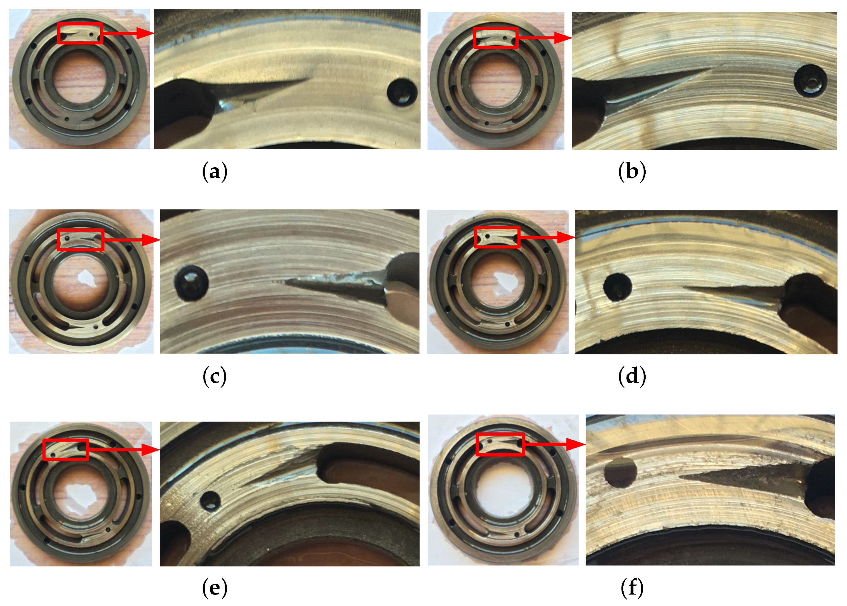
2.1. Selection of Degenerative Characteristics of Piston Pump

The signals can be adaptively decomposed into several IMFs with different center frequencies by the VMD. The analysis and processing of the original signal are essentially the calculation of the extreme value problem [40]. The calculation process is divided into two parts [41].
  • Establishment of variational problems.
    The analytical signals of each component function μ k (t) are obtained by Hilbert transform and the corresponding unilateral spectrum is calculated:
    φ ( t ) = [ δ ( t ) + j π t ] μ k ( t )
    where, the meaning of * is convolution operation. By parsing the signals in each component, center frequencyis e j ω k t is mixed and estimated. Adjust the spectrum of each component to its respective baseband:
    σ ( t ) = φ ( t ) e j ω k t
    Estimating the frequency range of each component signal, the variational problem when constrained is as follows:
    min { u k } , { ω k } k t δ t + j π t u k ( t ) e j ω k t 2 s . t . k u k = f
    where, u k = u 1 , u 2 , , u n , ω k = ω 1 , ω 2 , , ω n .
  • Analytical processing.
    Introducing the Lagrange multipliers λ (t) and the penalty factor α to transform the constrained variational problem into an unconstrained variational problem. Where λ (t) can keep the constraints rigorous, α can ensure the reconstruction accuracy of the signals when the signals contained Gaussian noise. The extended Lagrangian expression is as follows:
    L u k , ω k , λ = α k t δ t + j π t u k ( t ) e j ω k t 2 2 + f ( t ) k u k ( t ) 2 2 + λ ( t ) , f ( t ) k u k ( t )
    Solving it by the alternating directions method of multipliers, alternately update μ k n + 1 , ω k n + 1 and λ t n + 1 to find the critical point in the extended Lagrangian expression that is neither a maximum nor a minimum. The task consists of the following steps:
    • Initialize { μ k 1 } , { ω k 1 } , λ 1 , and n = 1.
    • Update μ k , ω k , according to Equations (5) and (6).
      u k n + 1 ( ω ) = f ( ω ) i k u i ( ω ) + λ ( ω ) 2 1 + 2 α ( ω ω k ) 2
      ω k n + 1 = 0 ω u k ( ω ) 2 d ω 0 u k ( ω ) 2 d ω
    • Update λ , according to λ n + 1 = λ n + τ ( f ) μ k n + 1 .
    • Repeat steps b and c, for the given discrimination precision e > 0, If stop iteration and get IMFs.
      k u k n + 1 u k n 2 2 k u k n 2 2 < e
In this paper, a MPE method was proposed based on PE, which can select multiple time series of different lengths and solve the entropy value [21,25]. The principle is as follows:
The time series x ( i ) are processed in multi-scale to obtain multi-scale sequence y j ( l ) .
y j ( l ) = 1 l i = ( j 1 ) l + 1 j l x i
where l represented the scale factor, l = 1, 2, …, [N/l], [N/l] represented the rounding of N/l. The l determines the multi-scale degree of the time series. When l = 1, the multi-scaled time series obtained is the original time series.
After dividing the time series into different data lengths, the MPE can be obtained by calculating the PE of all time series of different lengths [42]. The length of the divided time series does not affect its entropy calculation, so the value of the scale factor l is generally greater than or equal to 10.

2.2. Binary Gaussian Process Classification

Let the training sample be D = ( X , y ) , where X are the sample set of input features and y = { y 1 , y 2 , y i } are the category Labels. The general process of Gaussian process classification [43] is as follows:
Suppose the prior distribution of the implicit function f ( X ) = { f 1 , f 2 , , f i } is normal distribution, so:
p ( f | X ) : N ( f | m , K )
where K is an m-order covariance matrix that is symmetric and positive definite, Hyper parameters of K , estimated by maximum likelihood method, m = E [ f ( X ) ] is expressed as its mean function, Potential function value is f i = f ( X i ) , The class label y is independently identically distribution. The probability that the sample X i belongs to the class label in the Binary Classification of Gauss Process can be expressed as:
p ( y i | f i ) = S i g ( y i f i )
The function of the S i g ( ) is to convert the output value into a probability to find the probability that the input data belongs to a certain class. S i g ( ) is a response function whose value is between intervals [0, 1], thereby obtaining a likelihood function:
p ( y | f ) = i = 1 n p ( y i | f i ) = i = 1 n S i g ( y i f i )
The posterior probability of f can be obtained by Bayesian formula:
p ( f | X , y ) = p ( y | f ) p ( f | X ) P ( y | X )
In summary, for the specified data X # , its posterior probability of f # is expressed as:
p ( f # | X , y , X # ) = p ( f # | f , X , X # ) p ( f | X , y ) d f
Furthermore, the classification prediction probability corresponding to f # is deduced as:
p ( y # | X , X # , y ) = S i g ( y # f # ) p ( f | X , y ) d f #
In the GPC model, p ( y # | X , X # , y ) = 0.5 is often used as the classification boundary. When y > 0.5, y # = +1, on the contrary, y # = −1.

2.3. Gaussian Process Regression

Let D = { ( x i , y i ) | i = 1 , 2 , n } = ( X , y ) be a known data, where X = ( x 1 , x 2 , , x i ) is a matrix of d × n dimensions, y i is the output data corresponding to it, and y is a vector set of y i . The purpose of the regression process is to establish a mapping relationship between the vector set X and the vector set y by analyzing the known data set, and finally realize the prediction of the matching the unknown input value [44]. The equation of Gaussian process is:
f ( X ) G P ( m ( X ) , k ( X , X ) )
where, m ( X ) is mean function and k ( X , X ) is the kernel function, k ( X , X ) = E [ ( f ( X ) m ( X ) ) ( f ( X ) m ( X ) ) ] .
To consider the influence of noise on the observation target y, establish a general model of GPR [45]:
y f ( X ) + ε
where ε is an independent Gaussian white noise, which is Gaussian-distributed, with a mean of 0 and a variance of σ 2 . Since the noiseis white noise independent of f ( X ) , when f ( X ) obeys the Gaussian distribution, y also obeys the Gaussian distribution, then the set of joint distributions can form a Gaussian process, which can be expressed as:
y G P ( m ( X ) , k ( X , X + σ n 2 δ i j ) )
According to the Bayesian principle, GP establishes a priori function in a given data set D , and converts to a posterior distribution under n given test data sets D 1 , then the joint Gaussian distribution between the output vector y of the training data vector X and the output vector y of the test data X can be expressed as:
y y N 0 , K ( X , X ) + σ n 2 I K ( X , X ) T K ( X , X ) K ( X , X )
This gives a GPR equation, which can be expressed as:
p ( y X , X , y ) = N [ K ( X , X ) [ K ( X , X ) + σ n 2 I ] 1 y , K ( X , X ) K ( X , X ) [ K ( X , X ) + σ n 2 I ] 1 K ( X , X ) ]

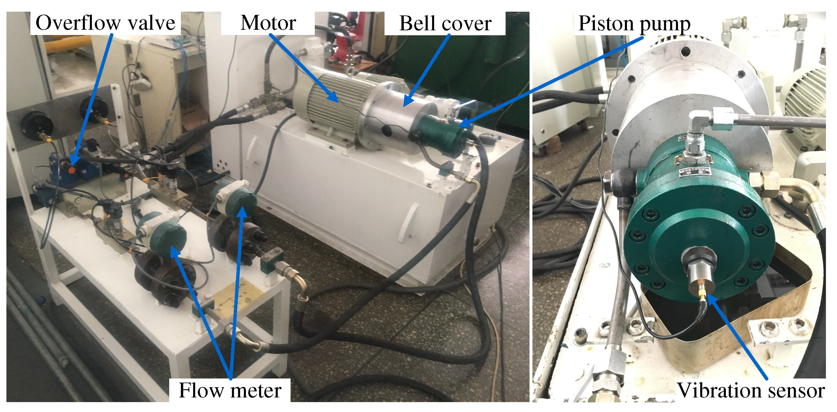
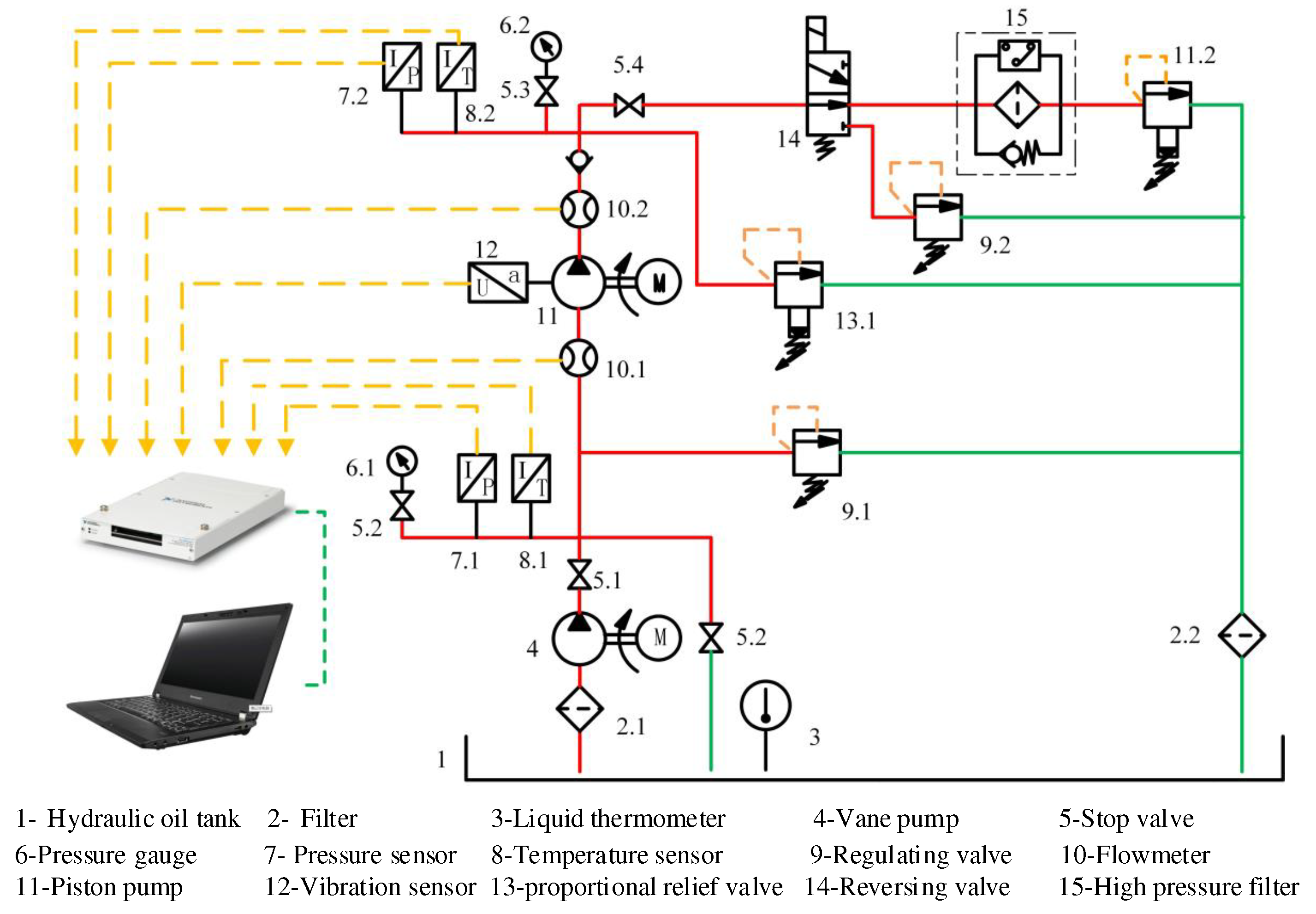
3. Performance Degradation Test of Axial Piston Pump

The field work picture of the test bench is illustrated in Figure 2. Figure 3 is a hydraulic system diagram of the performance degradation test about the axial piston pump. The vane pump was used as a slippage pump to make up oil for the hydraulic system, so as to improve the inadequate self-priming ability of the axial piston pump when the valve plate was seriously worn. During the test, the vibration acceleration sensor was placed at the end cover of the piston pump to collect the vibration signal of the pump. Further, turbine flow meters were installed in the inlet and outlet ports of the piston pump to collect real-time pump flow signals. In the degradation test of axial piston pump, only the degradation of the valve plate took place.
The purpose of the experiment was to investigate the effect of a definite part of the axial piston pump on the performance degradation. The principal wearing parts of the valve plate are the auxiliary support surface of the high pressure area and the transition area of the distribution slots. In this experiment, different degradation states were obtained by wearing the transition area of the distribution slots with a grinding wheel. The degree of wearing will vary with the wear time.
In order to simulate the actual process that the degradation of valve plate affects the performance, the first valve plate was not treated, and the other five identical valve plates were artificially treated with different degrees of wear, then the different degradation states of valve plate were obtained. The valve plates with different wear degrees are showed in Figure 4. Finally, the experiment was carried out by changing the valve plate with different degrees of wear. In the experiment of each valve plate, the pilot relief valve was adjusted to make the system pressure 15 MPa all the time, and the sampling frequency of the signal acquisition system was set to 20 kHz and the sampling time to 8 s. In this way, vibration signals and flow signals of six degraded states were obtained.
From the wearing stages of the valve plates, it is seen that there are plough-like stripes on the working face of the valve plate. Wear degree of valve plate was measured by the profilometer as showed in Figure 5.
The stylus of the profilometer performed the slip measurement on the surface of the valve plate to map the shape of the surface contour curve. The depth of the working surface of the valve plate in different degraded states is shown in Table 1.

4. Test Data Processing Of Vibration Signals

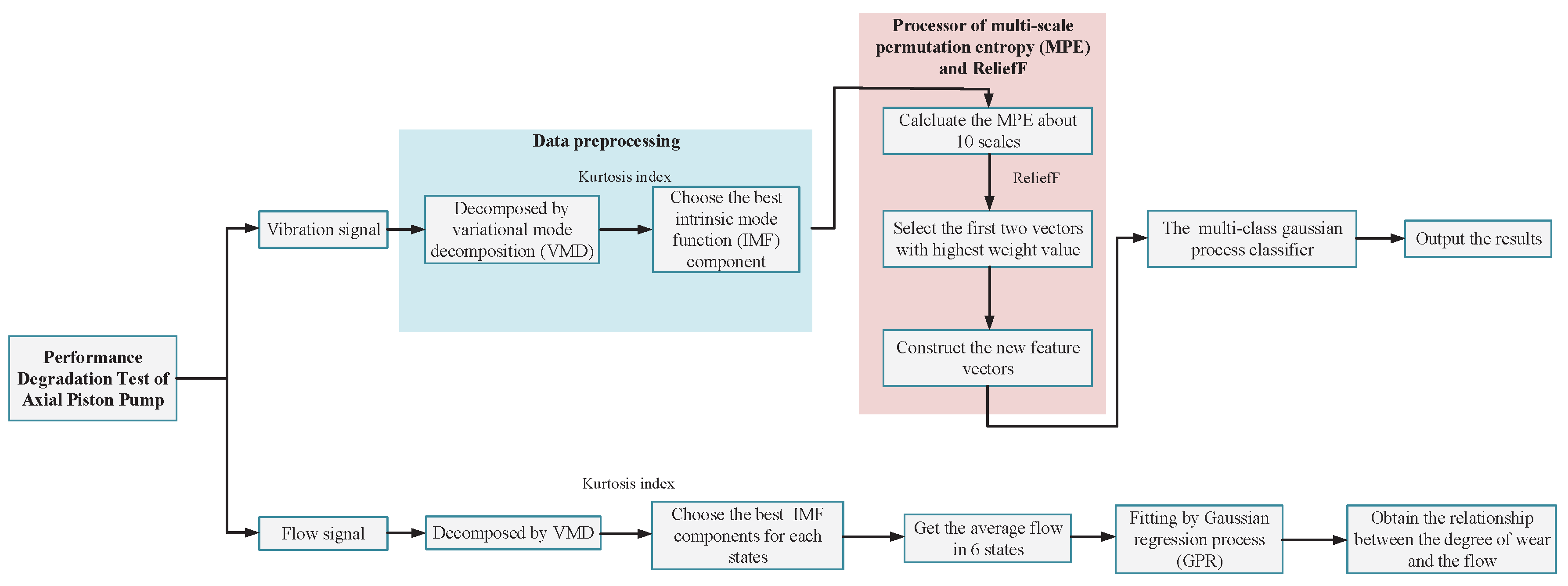
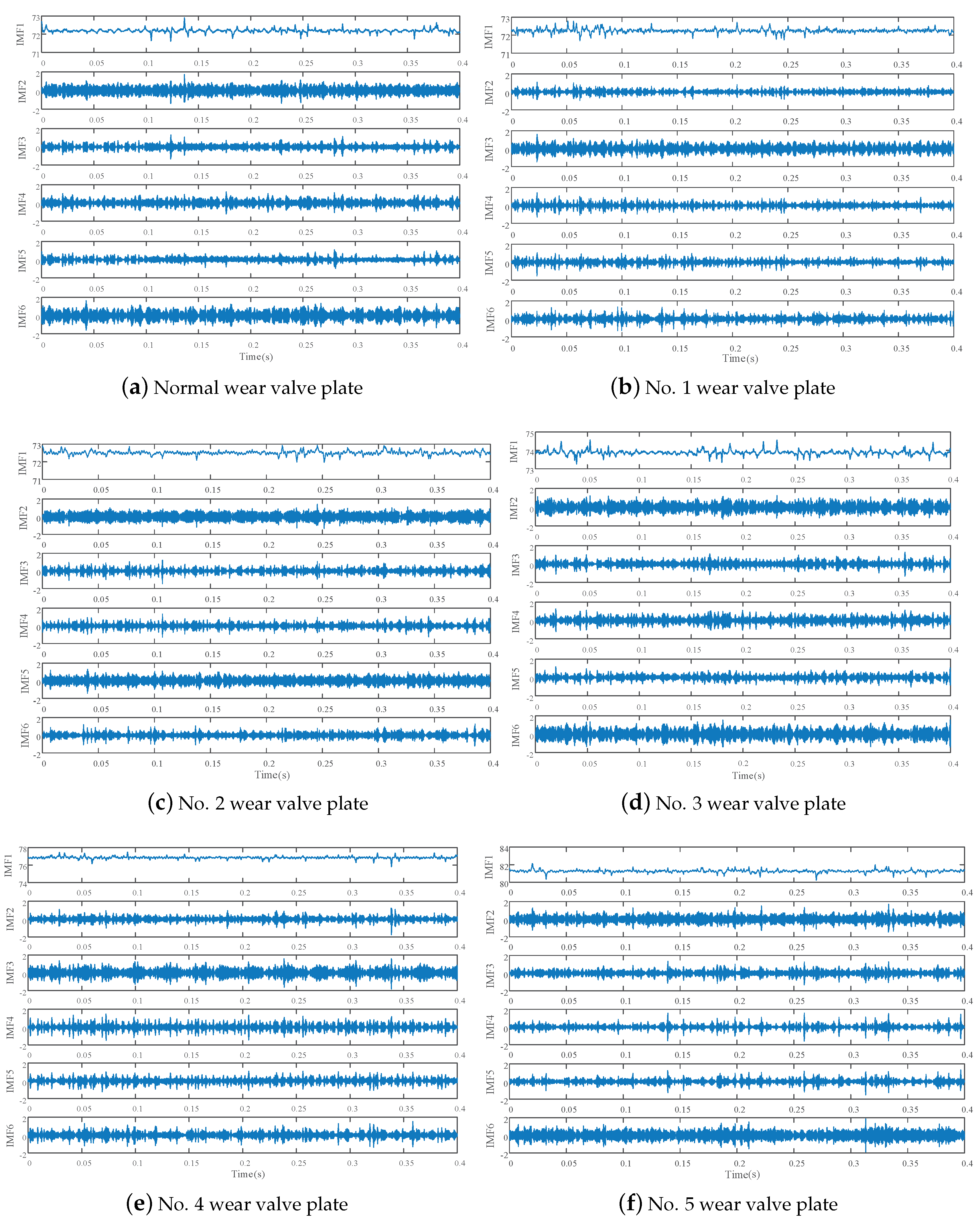
4.1. VMD-Based Test Data Processing

In this paper, the value of K in the VMD algorithm was set by observation method [46], and the center frequency of each component of the vibration signals was observed. If the center of gravity about the two components are small, it is deemed to be over-decomposed. Take the vibration signal when the valve plate was not worn as an example. When different values were taken by K, the center frequency of each IMF component was decomposed by VMD is given in Table 2.
It is be seen from the above table that when K = 7, an over-decomposition phenomenon with a similar center frequency occured, so the value of K is 6. Figure 6 shows a VMD exploded view of six status signals.
The kurtosis index [47] is a parameter commonly used to reflect characteristics of the time domain, which could well reflect the impact characteristics of vibration signals, it is defined as:
K v = 1 N i = 1 N ( x i x ¯ ) 4 / δ x 4
where, x i is the signal value, x ¯ is the signal mean value, N is the sampling length, and δ x is the standard deviation. Then kurtosis index was used to screen each IMF component of the vibration signals in six states, and selected the component with the largest kurtosis value. Kurtosis values of IMFs about the six states are shown in Table 3.
From the above table, the magnitude of each IMF component is seen in the 6 states. We selected the IMF3 of the normal valve plate’s vibration signal, the IMF6 of the No. 1 wear state, the IMF2 of the No. 2 wear degree, the IMF1 of the No. 3 wear degree, the IMF2 of the No. 4 wear degree, and the IMF1 of the No. 5 wear degree.

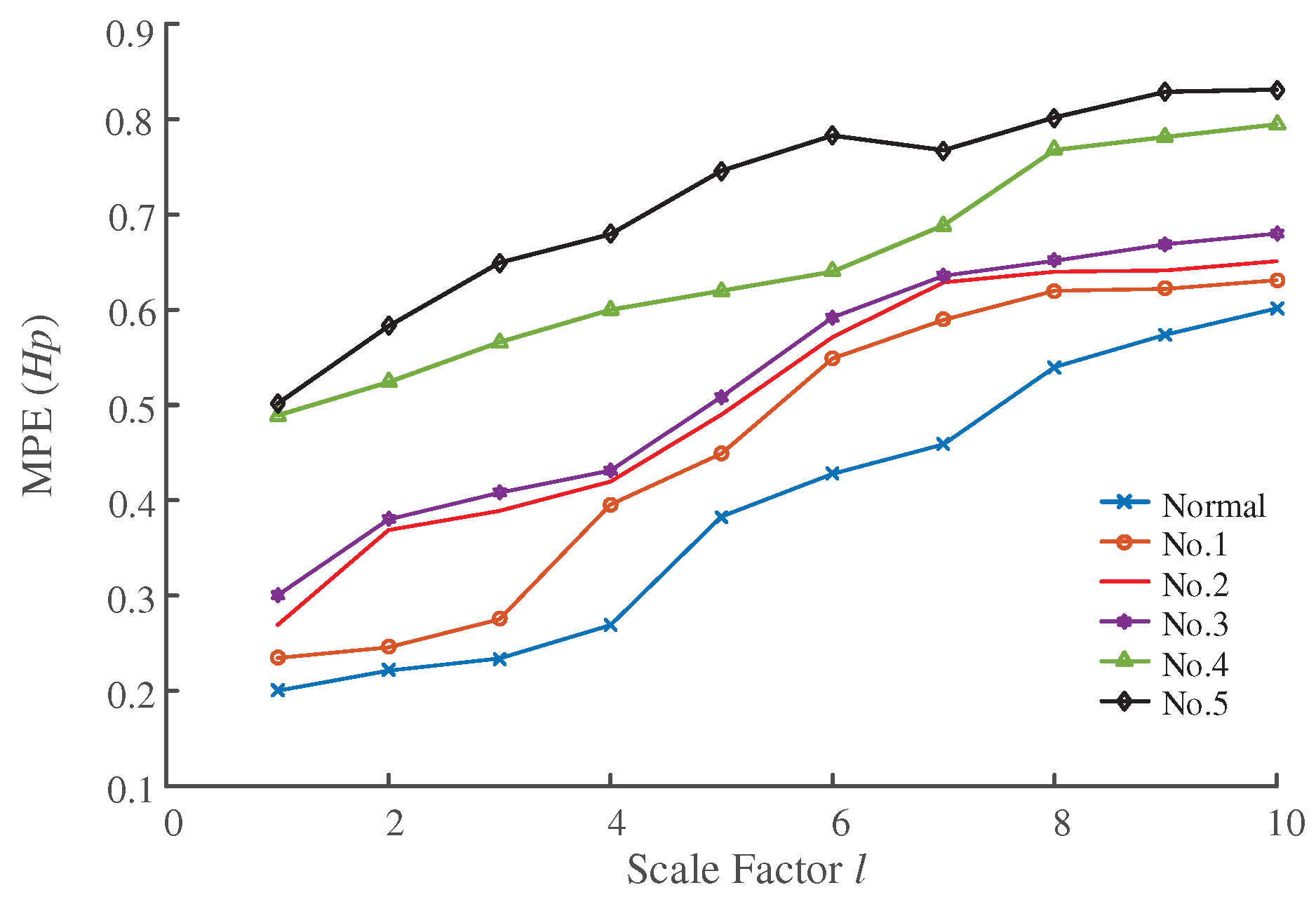
4.2. Feature Extraction Method Based on MPE

After the VMD and the kurtosis values processing, the selected IMFs in six degraded states were analyzed by MPE to extract feature vectors. Two key parameters of MPE, delay time parameter λ and embedding dimension m, were determined by mutual information and Cao’s method [48].
When the mutual information function obtained the minimum value for the first time, the corresponding time was selected as the value of delay time λ . The relationship between the delay time and the mutual information about selected IMFs is shown in Figure 7.
It is seen from Figure 7 that when the value of delay time was 1, the mutual information obtained the minimum value for the first time, so the delay time λ = 1. After determining the value, Cao’s method was used to select the value of embedding dimension m. The result is shown in Figure 8.
As could be observed in Figure 8 when m 6 , the value of E 1 ( m ) gradually became stable, so the embedding dimension m was taken as 6. Therefore, we analyzed the selected IMFs by MPE. Take λ = 1, m = 6, and selected the largest scale factor l to be 10. The MPE in different states is shown in Figure 9:
It can be observed in the figure that with the increase of scale factor, the degradation states of different degrees have obvious difference. The higher the degradation degree was, the higher the MPE value was. In the same state, with the increase of scale factor, the randomness and complexity of time series decreased, and the values of MPE tended to change smoothly. MPE distinguished the signals of different degraded state, so it was used as feature vectors to identify the state of the valve plate.
If 10 feature vectors are utilized to training, information redundancy will be caused and the training will be time-consuming. Therefore, the weights of feature vectors were calculated by using the ReliefF. The two feature vectors with the highest weight were selected, the results are shown in Figure 10. It is seen from the figure that different degradation states distinguish obviously.

4.3. Axial Piston Pump State Identification Based on Multi-Class Gaussian Process Classification

In this paper, multi-class Gaussian process classification model [49] was proposed. The essence of this classification model is to convert C different types of multi-classification into the sum of C two-category.
The training set D = ( X , y ) and test data X are assumed, where X = [ x 1 , x 2 , , x c ] T , y = [ y 1 , y 2 , , y c ] T , the test data X is respectively input into C two-class classifiers. Thereby obtaining C prediction probabilities, then the maximum prediction probability can be obtained from it. This maximum prediction probability means that X belongs to category(k). The specific steps are as follows:
  • In the training phase of the binary Gaussian process classification, the eigenvector data of the normal valve plate is marked as y i = 1 , the others are marked as y i = 1 . The first two-class classifier can be obtained by the Gaussian processes for binary classification used in Section 2.2.
  • The value of K is defined from 2 to 6 in turning. The training data of class K is indicated as y i = 1 and the other five training data are marked as K-class members of y i = 1 . Then, we get the training model of classifiers with different wear degrees, and finally six two-class classifiers are obtained.
  • The probability p k of the test data X belonging to the class K can be obtained by the above-mentioned six two-class classifiers respectively, and then a probability vector P = ( p 1 , p 2 , , p k ) is obtained. Finally, X can be classified as category (K) by maximum probability, which can be found from P .
In this paper, the feature vectors of vibration signals after VMD and MPE processing are selected. 50 sets of data samples were selected from each degradation state, 20 sets of data were used as training sets for multi-class Gaussian process classification model and 30 sets of data were used to test the accuracy of the model. Table 4 is a statistical table of classification accuracy rate.
From Table 4, only in the normal data and the No. 1 data, there is an error in the hydraulic pump data, but overall it has a good recognition effect. The recognition accuracy of multi-class Gaussian process classification is 98.9% (178/180).
In the same test environment and the same data, this paper introduced BP neural network [50] and SVM [51] method, compared the recognition accuracy and decision time with multi-class Gaussian process classification. The BP neural network is selected as three layers (two input neurons, nine hidden neurons, six output neurons). The kernel function of SVM is RBF, and two important parameters of SVM, penalty coefficient and gamma, are obtained by cross validation. Penalty coefficient is 4 and gamma is 0.1. The results are shown in the Table 5:
It can be seen from the table that the accuracy of BP neural network was the lowest, which was 92.8%, followed by that of SVM, which was 95.0%. Compared with the two algorithms, the accuracy of multi-class Gaussian process classification was more accurate. In terms of decision time, BP neural network took 3.135 s, SVM took 1.903 s, and multi-classification method based on Gaussian process took 1.257 s, so the running time of multi-class Gaussian process classification was the shortest. On the whole, no matter the decision time or recognition accuracy, the multi-class Gaussian process classification was more effective and comprehensive, which provides a new method for the degradation state identification of axial piston pump. In order to further prove the superiority and effectiveness of the methods proposed in this paper, some comparisons between the present work and the methods mentioned in the above literature using different methods were done. The comparative result is shown in Table 6.
The comparison results in Table 6 show that multi-class Gaussian process classification combined with VMD, MPE and ReliefF is a promising method for degradation state recognition.

5. Test Data Processing of Flow Signals

In the working process of hydraulic pump, the wear between the valve plate and the cylinder block will gradually increase with the increase of time, and irregular scratches will appear on the cross section of the valve plate and the cylinder block to increase the surface roughness. This results in poor coordination between the cylinder block and the valve plate, which can not form a stable and uniform oil film, and then under the action of high pressure, hydraulic oil leakage occurs, which increases the leakage flow rate. The relationship between the leakage flow caused by the wear of the valve plate and the cylinder block is calculated according to the following formula.
When the number of pistons in a piston pump is odd, the number of pistons that suck and discharge oil at different times is constantly changing, and the wrap angle of the oil distribution belt is also different [52]. When there are (z + 1)/2 pistons for oil discharge, the actual wrap ϕ 1 angle of the oil seal belts is calculated as follows:
ϕ 1 = z 1 2 α + α 0
When there are (z− 1)/2 pistons for oil discharge, the actual wrap angle of the oil seal belts is calculated as follows:
ϕ 2 = z 3 2 α + α 0
Then the average wrap angle is as follows:
ϕ p = z 2 2 α + α 0
where z is number of plungers, α 0 is wrapping angle of oil hole in piston chamber, α is the piston spacing angle. The formula for the total leakage of the axial piston pump is as follows:
q = φ 1 δ 3 p b 12 μ ln R 1 R 2 + φ 1 δ 3 p b 12 μ ln R 3 R 4
where δ is wear volume, μ is dynamic viscosity of hydraulic oil, p b is pressure at the outlet or suction port. ϕ 1 is actually wrapping angle of oil seal belt, R 1 , R 2 , R 3 and R 4 are sizes of inner and outer sealing oil belt of the valve plates.
Axial piston pump of 10MCY14-1B model was used, the actual sizes of valve plate are: R 1 = 25 mm, R 2 = 23 mm, R 3 = 19 mm, R 4 = 17 mm, Z = 7, α 0 = 60. By using the pressure sensor, the inlet pressure of axial piston pumps was 0.3 MPa. The flow signals were collected when working pressure of the axial piston pump was 15 MPa. After the end of test, the valve plates were removed and cleaned. The wear of valve plates were measured by a profiler, the measurement results are showed in Table 1.
Since the flow signal of the piston pump also has noise, the leakage flow signals with different wear degrees are denoised by VMD. The processing results are shown in Figure 11.
Then kurtosis index was used to filter the IMF component of the flow signal in the six states, and IMF components with the largest kurtosis value were selected. The average flow of the selected IMF components were calculated, and the results are shown in Table 7.

Failure Prediction of Axial Piston Pump

When the volumetric efficiency decreased by 5%, the axial piston pump failed. The fit curve of GPR is used to predict the wear of the valve plate in the failure of the piston pump. The result is shown in Figure 12. According to the Equation (24), the relationship between the wear of valve plates and the flow was established. The actual curve is as shown in Figure 12.
In order to evaluate the estimation effect, this paper introduced three evaluation indexes: square sum of error (SSE), root mean square error (RMSE) and correlation coefficient R 2 . The estimation error of GPR is showed in Table 8. It is seen from Table 8 that the GPR model is ideal for estimating the axial piston pump leakage flow curve.
According to the performance of 10MCY14-1B piston pump, when the volumetric efficiency decreased by 5%, the flow rate was 117.19 L/h. It is concluded from Figure 12, according to the theoretical calculation, that when the axis piston pumps failed, the wear amount of the valve plate was 12.8 μ m. According to the fitting curve of Gaussian process regression, when the axis piston pump failed, the wear amount of the valve plate was 12.4 μ m. By comparing the theoretical result with the predicted result, the Relative error was 3.125%. Therefore, the fitting curve of GPR in this paper had a good effect on the failure prediction by leakage of the axis piston pump.

6. Conclusions

In this paper, the wear of the valve plate, which is one of the key factors causing the failure of axial piston pump, is studied. The vibration signals and flow signals of the axial piston pump under wear conditions are collected by establishing the degradation test-bed. The following conclusions have been drawn:
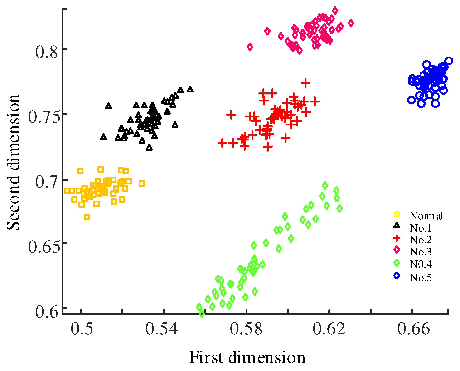
  • The combination of VMD, MPE, and ReliefF has obvious advantages in feature extraction. Moreover, the complexity and time of the operation are decreased by reducing the dimension of the feature. At the same time, the discrimination of the feature vectors in different degraded states is very high, and there is almost no overlap of data values.
  • The multi-class Gaussian process classification model is used to realize the state recognition, which has high accuracy and enriches the research on the vibration signals processing and analysis of axial piston pump. In the same test conditions, compared with the BP neural network and the SVM method, the multi-class Gaussian process classification provides a better recognition effect and shorter decision time.
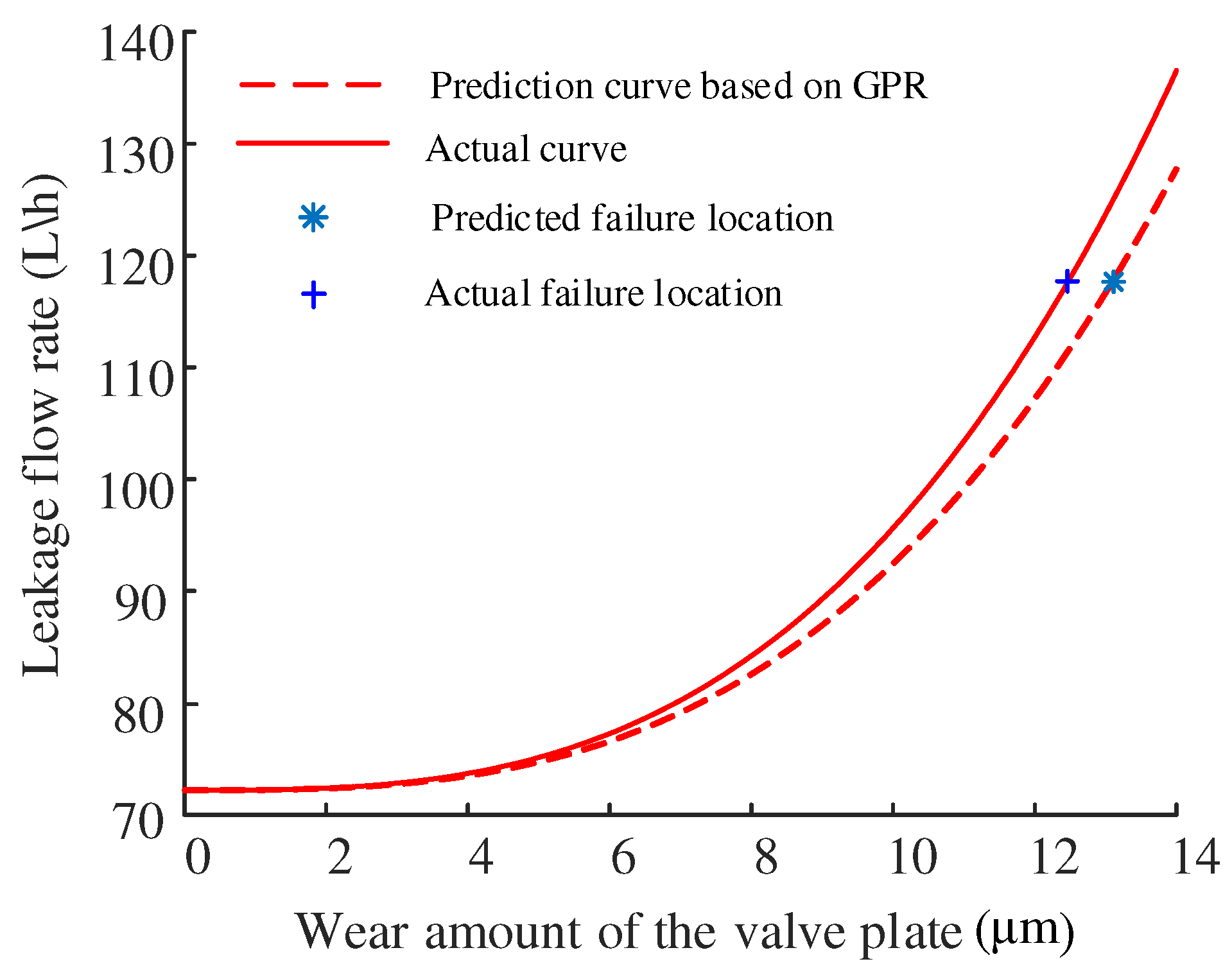
  • The mathematical model of the relationship between the flow and the wear of the valve plate is established by using the GPR, and compared with the actual curve to determine its superiority. Therefore, the failure prediction by GPR provides a new idea for the research on the relationship between the wear and failure of axial piston pump.

Author Contributions

All the authors contributed to the original idea and design of the study, to the analysis, to the drafting of the manuscript, reading and approving the final version. Conceptualization, R.G. and Z.Z.; methodology, R.G.; validation, R.G., S.H. and Z.Z.; formal analysis, Z.J. and D.G.; resources, R.G.; data curation, Z.Z.; writing–original draft preparation, Z.Z.; writing–review and editing, R.G. and Z.Z.; visualization, Z.Z.; Software, Z.J.; supervision, J.Z. and S.H.; project administration, Z.J. and R.G.; funding acquisition, J.Z., R.G. and D.G. All authors have read and agreed to the published version of the manuscript.

Funding

This research was funded by the National Key Research and Development Program of China (Grant No. 2019YFB2005204), the National Natural Science Foundation of China (Grant No. 51675461, 11673040), the Key Research and Development Program of Hebei Province (Grant No. 19273708D) and the Open Foundation of the State Key Laboratory of Fluid Power and Mechatronic Systems (Grant No. GZKF-201922).

Acknowledgments

The authors would like to acknowledge the support provided by Yanshan University.

Conflicts of Interest

The authors declare no conflict of interest.

References

  1. Stefan, G.; Hubertus, M. Simulation of the Lubricating Film between Contoured Piston and Cylinder. Int. J. Fluid Power 2010, 11, 15–24. [Google Scholar]
  2. Olems, L. Investigation of the Temperature Behavior of the Piston Cylinder Assembly in Axial Piston Pumps. Int. J. Fluid Power 2000, 1, 27–39. [Google Scholar] [CrossRef]
  3. Li, H.R.; Wang, Y.K.; Ma, J.Q.; Ye, P. Fault pattern recognition of hydraulic pumps based on MMSE and ABCSVM. J. Vib. Shock 2016, 35, 152–158. [Google Scholar]
  4. Lee, J.; Wu, F.; Zhao, W.; Ghaffari, M.; Liao, L.; Siegel, D. Prognostics and health management design for rotary machinery systems—Reviews, methodology and applications. Mech. Syst. Signal Process. 2014, 42, 314–334. [Google Scholar] [CrossRef]
  5. Zamanian, A.H.; Ohadi, A. Gear fault diagnosis based on Gaussian correlation of vibrations signals and wavelet coefficients. Appl. Soft Comput. J. 2011, 11, 4807–4819. [Google Scholar] [CrossRef] [Green Version]
  6. Lin, J.S.; Chen, Q. Fault diagnosis of rolling bearings based on multifractal detrended fluctuation analysis and Mahalanobis distance criterion. Mech. Syst. Signal Process. 2013, 38, 515–533. [Google Scholar] [CrossRef]
  7. Wang, Y.K.; Li, H.R.; Huang, Z.J. Transform Relative Spectrum Entropy and It Application in Degradation State Identification of Hydraulic Pump. Acta Armamentarii 2016, 37, 979–987. [Google Scholar]
  8. Li, N.; Zhou, R.; HU, Q.H.; Liu, X.H. Mechanical fault diagnosis based on redundant second generation wavelet packet transform, neighborhood rough set and support vector machine. Mech. Syst. Signal Process. 2012, 28, 608–621. [Google Scholar] [CrossRef]
  9. Zeng, Q.H.; Qiu, J.; Liu, G.J.; Tan, X.D. Research on equipment degradation state recognition and fault prognostics method based on KPCA-Hidden Semi-Markov Model. Chin. J. Sci. Instrum. 2009, 30, 1341–1346. [Google Scholar]
  10. Gao, Y.J.; Kong, X.D. Wavelet Packets Analysis Based Method for Hydraulic Pump Condition Monitoring. J. Mech. Eng. 2009, 45, 80–88. [Google Scholar] [CrossRef]
  11. Sun, J.; Li, H.R.; Tian, Z.K. A degradation feature extraction method for hydraulic pumps based on fusion of sensitive components. Chin. J. Sci. Instrum. 2016, 37, 1290–1298. [Google Scholar]
  12. Wang, S.P.; Wan, Z.K.; Yang, G.Q. Study on Fault Diagnosis of Data Fussion in Hydraulic Pump. China Mech. Eng. 2005, 5, 47–51. [Google Scholar]
  13. Wu, C.Q.; Jiang, W.L. Multi-source and multi-feature fused fault diagnosis on piston pumps based on evidence theory. Chin. J. Constr. Mach. 2011, 9, 98–102. [Google Scholar]
  14. Zhang, X.; Liang, Y.; Zhou, J.; Zang, Y. A novel bearing fault diagnosis model integrated permutation entropy, ensemble empirical mode decomposition and optimized svm. Measurement 2015, 69, 164–179. [Google Scholar] [CrossRef]
  15. Lu, C.; Wang, S.; Maids, V. Fault severity recognition of aviation piston pump based on feature extraction of eemd paving and optimized support vector regression model. Aerosp. Sci. Technol. 2017, 67, 105–117. [Google Scholar] [CrossRef]
  16. Wang, X.; Liu, C.; Bi, F.; Bi, X.; Shao, K. Fault diagnosis of diesel engine based on adaptive wavelet packets and eemd-fractal dimension. Mech. Syst. Signal Process. 2013, 41, 581–597. [Google Scholar] [CrossRef]
  17. Zhao, S.F.; Liang, L.; Xu, G.H.; Wang, J.; Zhang, W.M. Quantitative diagnosis of a spall-like fault of a rolling element bearing by empirical mode decomposition and the approximate entropy method. Mech. Syst. Signal Process. 2013, 40, 154–177. [Google Scholar] [CrossRef]
  18. Ji, N.; Ma, L.; Dong, H.; Zhang, X. EEG Signals Feature Extraction Based on DWT and EMD Combined with Approximate Entropy. Brain Sci. 2019, 9, 201. [Google Scholar] [CrossRef] [Green Version]
  19. Widodo, A.; Shim, M.C.; Caesarendra, W.; Yang, B.S. Intelligent prognostics for battery health monitoring based on sample entropy. Expert Syst. Appl. 2011, 38, 11763–11769. [Google Scholar] [CrossRef]
  20. Tan, J.; Fu, W.; Wang, K.; Xue, X.; Hu, W.; Shan, Y. Fault Diagnosis for Rolling Bearing Based on Semi-Supervised Clustering and Support Vector Data Description with Adaptive Parameter Optimization and Improved Decision Strategy. Appl. Sci. 2019, 9, 1676. [Google Scholar] [CrossRef] [Green Version]
  21. Bandt, C.; Pompe, B. Permutation Entropy: A Natural Complexity Measure for Time Series. Phys. Rev. Lett. 2002, 88, 174102. [Google Scholar] [CrossRef]
  22. Rolo, A. A method for the correlation dimension estimation for on-line condition monitoring of large rotating machinery. Mech. Syst. Signal Process. 2005, 19, 939–954. [Google Scholar] [CrossRef]
  23. Richman, J.S.; Randall, M.J. Physiological time-series analysis, using approximate entropy and sample entropy. Am. J. Physiol.-Heart Circ. Physiol. 2000, 278, H2039–H2049. [Google Scholar] [CrossRef] [PubMed] [Green Version]
  24. Si, L.; Wang, Z.; Liu, X.; Tan, C. A sensing identification method for shearer cutting state based on modified multi-scale fuzzy entropy and support vector machine. Engineering Applications of Artificial Intelligence. Eng. Appl. Artif. Intell. 2019, 78, 86–101. [Google Scholar] [CrossRef]
  25. Yan, R.; Liu, Y.; Gao, R.X. Permutation entropy: A nonlinear statistical measure for status characterization of rotary machines. Mech. Syst. Signal Process. 2019, 29, 474–484. [Google Scholar] [CrossRef]
  26. Li, D.; Li, X.; Liang, Z.; Voss, L.J.; Sleigh, J.W. Multiscale permutation entropy analysis of eeg recordings during sevoflurane anesthesia. J. Neural Eng. 2010, 7, 046010. [Google Scholar] [CrossRef] [PubMed]
  27. Bect, P.; Simeu-Abazi, Z.; Maisonneuve, P.L. Diagnostic and decision support systems by identification of abnormal events: Application to helicopters. Aerosp. Sci. Technol. 2015, 46, 339–350. [Google Scholar] [CrossRef]
  28. Zheng, S.; Liu, W. An experimental comparison of gene selection by lasso and dantzig selector for cancer classification. Comput. Biol. Med. 2011, 41, 1033–1040. [Google Scholar] [CrossRef]
  29. Jaffel, I.; Taouali, O.; Harkat, M.F.; Messaoud, H. Kernel principal component analysis with reduced complexity for nonlinear dynamic process monitoring. Int. J. Adv. Manuf. Technol. 2016, 88, 9–12. [Google Scholar] [CrossRef]
  30. Zhang, J.; Chen, M.; Zhao, S.; Hu, S.; Shi, Z.; Cao, Y. ReliefF-Based EEG Sensor Selection Methods for Emotion Recognition. Sensors 2016, 16, 1558. [Google Scholar] [CrossRef]
  31. Jiang, W.L.; Wang, Y.R.; Wang, Z.W.; Zhu, Y. Fault Feature Dimension Reduction Method Combined ReliefF Algorithm with Correlation Calculation and Its Application. Chin. Hydraul. Pneum. 2015, 12, 18–24. [Google Scholar]
  32. Bevilacqua, M.; Braglia, M.; Montanari, R. The classification and regression tree approach to pump failure rate analysis. Reliab. Eng. Syst. Saf. 2003, 79, 59–67. [Google Scholar] [CrossRef]
  33. Turksoy, K.; Roy, A.; Cinar, A. Real-time model-based fault detection of continuous glucose sensor measurements. IEEE Trans. Biomed. Eng. 2016, 64, 1437–1445. [Google Scholar] [CrossRef] [PubMed]
  34. Saravanan, N.; Ramachandran, K.I. Incipient gear box fault diagnosis using discrete wavelet transform (DWT) for feature extraction and classification using artificial neural network (ANN). Expert Syst. Appl. 2010, 37, 4168–4181. [Google Scholar] [CrossRef]
  35. Wang, S.; Xiang, J.; Zhong, Y.; Tang, H. A data indicator-based deep belief networks to detect multiple faults in axial piston pumps. Mech. Syst. Signal Process. 2018, 112, 154–170. [Google Scholar] [CrossRef]
  36. Ji, Y.; Sun, S. Multitask multiclass support vector machines: Model and experiments. Pattern Recognit. 2013, 46, 914–924. [Google Scholar] [CrossRef]
  37. Riihimki, J.; Jylnki, P.; Vehtari, A. Nested expectation propagation for Gaussian process classification. J. Mach. Learn. Res. 2013, 14, 75–109. [Google Scholar]
  38. Wei, Z.; Wang, Y.; He, S.; Sao, J. A novel intelligent method for bearing fault diagnosis based on affinity propagation clustering and adaptive feature selection. Knowl. Based Syst. 2017, 116, 1–12. [Google Scholar] [CrossRef]
  39. Park, C.; Huang, J.Z.; Ding, Y. Domain decomposition approach for fast Gaussian process regression of large spatial data sets. J. Mach. Learn. Res. 2011, 12, 1697–1728. [Google Scholar]
  40. Dragomiretskiy, K.; Zosso, D. Variational mode decomposition. IEEE Trans. Signal Process. 2014, 62, 531–544. [Google Scholar] [CrossRef]
  41. Zhang, M.; Jiang, Z.; Feng, K. Research on variational mode decomposition in rolling bearings fault diagnosis of the multistage centrifugal pump. Mech. Syst. Signal Process. 2017, 93, 460–493. [Google Scholar] [CrossRef] [Green Version]
  42. Wang, Y.K.; Li, H.R.; Ye, P. Fault Identification of Hydraulic Pump Based on Multi-scale Permutation Entropy. China Mech. Eng. 2015, 26, 518–523. [Google Scholar]
  43. Kuss, M.; Rasmussen, C.E.; Herbrich, R. Assessing Approximate Inference for Binary Gaussian Process Classification. J. Mach. Learn. Res. 2005, 6, 1679–1704. [Google Scholar]
  44. Sun, B.; Yao, H.; Liu, T. Short-term wind speed forecasting based on Gaussian process regression model. Proc. Chin. Soc. Electr. Eng. 2012, 32, 104–109. [Google Scholar]
  45. He, Z.H.; Liu, G.B.; Zhao, X.J.; Wang, M.H. Overview of Gaussian process regression. Control Decis. 2013, 28, 1121–1129. [Google Scholar]
  46. Wu, M.; Feng, Z.; Huang, G.Y.; Mou, Z.Q. Early fault diagnosis of check valve based on variational mode decomposition and Wigner-Ville. China Meas. Test 2019, 45, 116–122. [Google Scholar]
  47. Decarlo, L.T. On the meaning and use of kurtosis. Psychol. Methods 1997, 2, 292–307. [Google Scholar] [CrossRef]
  48. Zheng, J.D.; Cheng, J.S.; Yang, Y. Multi-scale Permutation Entropy and Its Application to Rolling Bearings Fault Diagnosis. China Mech. Eng. 2013, 24, 2641–2646. [Google Scholar]
  49. Wei, S.X.; Sun, Z.H. A Multi-Classification Method Based on Gaussian Processes. Appl. Mech. Mater. 2012, 6, 1333–1337. [Google Scholar] [CrossRef]
  50. Wong, W.K.; Yuen, C.W.M.; Fan, D.D. Stitching defect detection and classification using wavelet transform and BP neural network. Expert Syst. Appl. 2009, 36, 3845–3856. [Google Scholar] [CrossRef]
  51. Abbasion, S.; Rafsanjani, A.; Farshidianfar, A. Rolling element bearings multi-fault classification based on the wavelet denoising and support vector machine. Mech. Syst. Signal Process. 2007, 21, 2933–2945. [Google Scholar] [CrossRef]
  52. Xie, J.H.; Liu, J.; Shang, J. Analysis and Calculation of Leakage of Swash-plate Axial Piston Pump. Fluid Mach. 2016, 44, 55–58+70. [Google Scholar]
Figure 1. Flow chart of technical route.
Processes 08 00609 g001
Figure 2. Test bench physical map.
Processes 08 00609 g002
Figure 3. Hydraulic system diagram of the performance degratation test of the piston pump.
Processes 08 00609 g003
Figure 4. Valve plates in six different wear states. (a) Normal valve plate and local amplification of its transition area. (b) No. 1 valve plate and local amplification of its transition area. (c) No. 2 valve plate and local amplification of its transition area. (d) No. 3 valve plate and local amplification of its transition area. (e) No. 4 valve plate and local amplification of its transition area. (f) No. 5 valve plate and local amplification of its transition area.
Processes 08 00609 g004
Figure 5. The profilometer measures the wear degree of valve plate on site.
Processes 08 00609 g005
Figure 6. VMD decomposition results of vibration signals in six states.
Processes 08 00609 g006
Figure 7. Relation of mutual information and delay time.
Processes 08 00609 g007
Figure 8. The curve of the embedding dimension.
Processes 08 00609 g008
Figure 9. MPE in different degenerate states.
Processes 08 00609 g009
Figure 10. The result of feature vector selection.
Processes 08 00609 g010
Figure 11. VMD decomposition results of flow signals in six states.
Processes 08 00609 g011
Figure 12. Gaussian Process regression fit curve.
Processes 08 00609 g012
Table 1. Wear scale of five different degrees of wear valve plates.
Wear Distribution PlateNo. 1No. 2No. 3No. 4No. 5
Maximum wear ( μ m)27121822
Average wear ( μ m)0.672.33467.3
Table 2. Center frequencies corresponding to different K values.
KCenter Frequency
22891484
328810612194
419534114512261
5195341106818432608
61953411039157322082880
71843398581421217728802883
Table 3. Kurtosis values of the modal components of the six states.
Status of Valve PlateIMF1IMF2IMF3IMF4IMF5IMF6
Normal3.92033.84844.12373.96984.00624.0229
No. 12.06802.15772.23452.11813.48823.5078
No. 22.06513.19141.58232.90042.49642.3559
No. 33.60371.61572.36952.65941.53501.5569
No. 41.84102.78261.68821.96282.39812.5837
No. 53.19683.02513.03953.65641.65813.1946
Table 4. Recognition accuracy of multi-class Gaussian process classification.
Number of SamplesNumber of Test SamplesIdentify the NumberRecognition Accuracy
Normal2030290.967
No. 12030290.967
No. 22030301
No. 32030301
No. 42030301
No. 52030301
Table 5. Comparison of degradation state recognition results.
Classification MethodCorrect IdentificationsRecognition Accuracy (%)Decision Time (s)
back propagation (BP)
neural network
16792.83.135
support vector machine (SVM)17195.01.903
Multi-class Gaussian
process classification
17898.91.257
Table 6. A comprehensive study between the current work and some recent publications.
ReferenceFeature
Extraction Method
Feature
Reduction Method
Classification TechniqueRecognition
Rate (%)
[6]empirical mode
decomposition (EMD),
wavelet transform (WT),
multifractal detrended
fluctuation analysis
(MF-DFA)
Mahalanobis
distance criterion
94.4–100
[7]Smooth Processing,
Transform Relative
Spectrum Entropy
weighted grey
correlation
88.8
[8]redundant
second-generation
wavelet packet
transform (RSGWPT)
neighborhood
rough set (NRS)
SVM93.9
[9]wavelet correlation
feature scale
entropy (WCFSE)
Kernel Principal
component
analysis (KPCA)
hidden
Semi–Markov
model(HSMM)
90
[12]WT, time domain,
frequency domain,
time-frequency domain
principal component
analysis (PCA)
BP neural network89.4–94.4
[14]ensemble empirical
mode decomposition
(EEMD),
Permutation entropy
SVM93.4–98.3
[15]EEMD, correlation
coefficient method,
time domain,
frequency domain,
time-frequency domain
PCAsupport vector
regression (SVR)
97.8–100
Present workVMD, Kurtosis and MPEReliefFmulti-class Gaussian
process classification
98.9
Table 7. Average flow in 6 states.
Valve PlateNormalNo. 1No. 2No. 3No. 4No. 5
Average flow (L/h)72.186972.244772.510073.885376.856981.2677
Table 8. Gaussian process regression estimation error table.
Evaluation IndexSSERMSE R 2
Gaussian regression0.11140.13620.9991

