Progressive System: A Deep-Learning Framework for Real-Time Data in Industrial Production

Abstract

Deep learning based on a large number of high-quality data plays an important role in many industries. However, deep learning is hard to directly embed in the real-time system, because the data accumulation of the system depends on real-time acquisitions. However, the analysis tasks of such systems need to be carried out in real time, which makes it impossible to complete the analysis tasks by accumulating data for a long time. In order to solve the problems of high-quality data accumulation, high timeliness of the data analysis, and difficulty in embedding deep-learning algorithms directly in real-time systems, this paper proposes a new progressive deep-learning framework and conducts experiments on image recognition. The experimental results show that the proposed framework is effective and performs well and can reach a conclusion similar to the deep-learning framework based on large-scale data.

1. Introduction

With the rapid development of artificial intelligence, intelligent manufacturing has become a hot topic in the industrial control field. Among them, fault diagnoses in industrial production processes have important significance in improving the production efficiency, ensuring the product quality, and maintaining employee safety. The fault diagnosis of the industrial production process has the characteristics of strong timeliness and complicated data structures. The traditional diagnosis method relying on manual experience is subjective and inaccurate. The emergence of data mining technology has promoted the research of abnormal diagnosis technology based on deep learning.

However, deep learning is often dependent on a large number of high-quality data, and once the data condition is not satisfied, it often leads to the following common questions:

(1) insufficient data: leading to underfitting problems—that is, the model cannot be effectively trained, and

(2) too much data: This leads to overfitting problems—that is, model training becomes more difficult, and it is easy to fall into a local optimum.

Data has become an important factor restricting the use of deep learning. Therefore, considering the characteristics of difficult image acquisition and high real-time requirements in industrial production, it is of great significance to propose a new image-processing technology based on deep learning.

This paper in the TensorFlow platform uses Google’s Inception-V3 convolution neural network [1] (Convolutional Neural Network, CNN) model to simulate the real-time image recognition system as an example to verify; experimental results show that the proposed framework and method is effective.

2. Related Work

2.1. Machine-Learning and the Processing of Small-Scale Data

Machine-learning, the human desire to endow the computer with the ability to solve specific problems through a specific algorithm, originated in the 1950s; it is one of the most important areas of artificial intelligence research. In 2006, Hinton proposed machine-learning based on deep neural networks to solve problems, and defined it as deep learning [2] (Deep learning, DL). This also marks the rise of deep learning. Deep learning not only can be applied to many areas, including pattern recognition, natural language processing, computer vision, speech processing, data mining, etc., but also greatly promote the development of these industries.

Currently, in the field of computer vision, whether it is engineering or academia, when faced with problems caused by data, the main methods adopted are:

(1) Insufficient amount of data: Create new data and increase the amount of data through a series of data-enhancement methods such as flipping, panning, and adding noise [3].

(2) Overfitting caused by too much data: Regularization [4], which suppresses the overfitting caused by data by adding regular terms after the loss function. Dropout [5], which reduces parameters in neurons to suppress overfitting altogether.

The problem of overfitting caused by the large amount of data has been well-mitigated, but in the objective situation where the amount of data is not large enough, the results obtained by using these methods are still limited. The 3D image is transformed by combining differential geometry and other methods, which only reduces the computational complexity of the image in pattern recognition to a certain extent [6]. Therefore, how to make small-scale data have the same effect as a large amount of data in data mining has become a new research hotspot in deep learning.

At present, in many real-time systems, we often want to process data efficiently by using a method of deep study in order to achieve judgment. However, due to problem such as in the system, data is generated in real time, and the amount of data generated each time is too small, the use of deep-learning methods is not effective and cannot even be used directly. In the absence of reliable data for an effective systems analysis, if the generated data is retained and saved until the amount of data is large enough to analyze, on the one hand, it will lose the timeliness of the data, making the analysis result inaccurate, and on the other hand, it will not meet the system’s real-time analysis requirements. Therefore, the amount of data has become an important factor restricting the use of deep learning to deal with the effective classification of data in real-time systems. Therefore, in the case of a limited amount of data, whether a reliable deep-learning framework can be adopted to complete the analysis of the data within a certain accuracy range is very important.

Aiming at the problem of poor performance in deep-learning frameworks due to the small amount of data, this paper proposes a progressive deep-learning framework for real-time data. The framework adopts a statistical-processing method for the results to ensure the reliability of the conclusions in the case of a limited data volume. At the same time, a model update strategy is proposed, which further improves the accuracy and stability of the model.

2.2. CNN and TensorFlow Platform

2.2.1. CNN and Inception-V3

Convolutional neural network (CNN) is widely applied to the field of preprocessing the image recognition, natural language processing, and the feed-forward neural network. Its neurons can respond to a part of the neurons it is connected to, so it performs well on image classification problems.

A typical CNN consists of an input layer, a convolutional layer, a pooling layer, a fully connected layer, and an output layer, as shown in Figure 1. First, different features in the image are extracted by convolutional layers and activation functions. Then, the features of the image are mapped to a high-dimensional space through the pooling layer to distinguish them, while reducing the amount of parameters. Through the combination of multiple convolutional layers and pooling layers, different feature regions in the image can be distinguished. Then, for specific classification tasks, whether to add a fully connected layer to learn global features is selected to achieve the image recognition classification problem.

Figure 1. This is a typical convolutional neural network (CNN).

Inception-V3 [7] is the third version of the GoogLeNet architectures proposed by Google. The Inception model uses a large number of 1 × 1, 3 × 3, and 5 × 5 convolution kernels, which widens the width of the neural network, greatly reduces the amount of parameters, and makes the model’s output of image classification results more obvious. There is good performance in the image recognition.

2.2.2. TensorFlow Framework Introduced

TensorFlow is the Google company’s proposed deep-learning platform, with a high degree of flexibility, portability, and rich library of algorithms.

Either a personal PC or a large-scale computing cluster GPU can be deployed in TensorFlow to perform calculations. At the same time, the trained model can be migrated between different devices at any time. The provided API (Application Programming Interface) basically meets most of the requirements. At the same time, you can also write the underlying algorithms yourself and add them to TensorFlow to solve different problems in different ways.

In the TensorFlow programming system, computing tasks are represented in the form of a graph, and the nodes in the graph are called op (operation). Each node can get zero, one, or more tensors, and each tensor is a multidimensional array. A typical TensorFlow framework is shown in Figure 2.

Figure 2. The framework of progressive deep learning.

3. Framework Introduction and Implementation Plan

3.1. Framework Introduction

The core idea of the model comes from the idea of combining mathematical statistics tools with human cognitive learning methods. There are good examples of combining statistical models with specific frameworks or platforms [8]. Human beings can obtain a more comprehensive and objective understanding of the matter through the description of the same thing by multiple absolutely objective people, thus getting their own assessment of the matter.

In this model, it is similar to the case where multiple people make limited observations of the same thing from different perspectives. Although everyone’s awareness of the problem is limited, and observation is not comprehensive, due to the number of factors, the problem of insufficient personal observation is made up. In the framework, the model trained with a small amount of data generated by the real-time system batch plays these absolute objective roles.

The whole frame consists of 3 parts, as shown in Figure 2.

$TrainData$ and $TrainedModel$: The training data of different batches are entered into the training framework of the model, and the corresponding $TestModel$ can be obtained.

$$TestMode{l}_i,i(1,n)$$

(1)

where $TestModel$ represents the corresponding model, $i$ represents the corresponding batch, and $n$ represents the total number of models.

$TestData$: Pass the test data to $TestMode{l}_j$ in turn and record the R after the test:

$$R=[\mathrm{Re}sul{t}_1,\mathrm{Re}sul{t}_2,\mathrm{Re}sul{t}_3,\cdots \mathrm{Re}sul{t}_i]$$

(2)

$ModelUpdate$: $\mathrm{Re}sul{t}_i$ is statistically calculated in order, and the model is updated in such a way that the worst results are automatically eliminated every k results.

3.2. Data Collection

The data is collected and obtained from the real-time system. When each batch of data is valid and classified correctly and clearly, it can enter the framework for training to obtain the model of the corresponding batch. However, in actual situations, the obtained data may not be all clear and available. The data entering the framework needs to be processed in advance to ensure the effectiveness of the training model and maintain the stability of the framework. The pseudo code of the framework data-cleaning Algorithm 1 is as follows:

Algorithm 1. Data preprocessing algorithm

Inputs: the training data $DataSet[i]$ that entered the framework, the amount of data Num, and the data label $DataSet[i].Label$.   Outputs: cleaned data set $DataSet[i]$. FOR i→1 TO NUM   1) IF !DataSet[i].Label OR UNCLEAR     I DELETE(DateSet[i])   II J++   2) END IF END FOR tmpNum=i-J IF tmpNum<Num     1) SAVE(DataSet) END IF ELSE     1) TRAIN(DataSet)

In the above data-cleaning process, the labels of each data in the current data set are identified and judged. When the data has no labels or the labels are not clear, the data is removed from the data set. Repeat the above process until every data has been processed. It is then determined whether the amount of data in the cleaned data set is sufficient for a round of training. If the amount of data is sufficient, train; otherwise, save the data to the next round of datasets and enter the merge to train together.

The robustness and stability of the framework proposed in this article are inferior to traditional deep-learning frameworks based on large amounts of data, so the requirements for the source of the data are relatively high, and the data-cleaning and filtering stages are an effective preprocessing of the data.

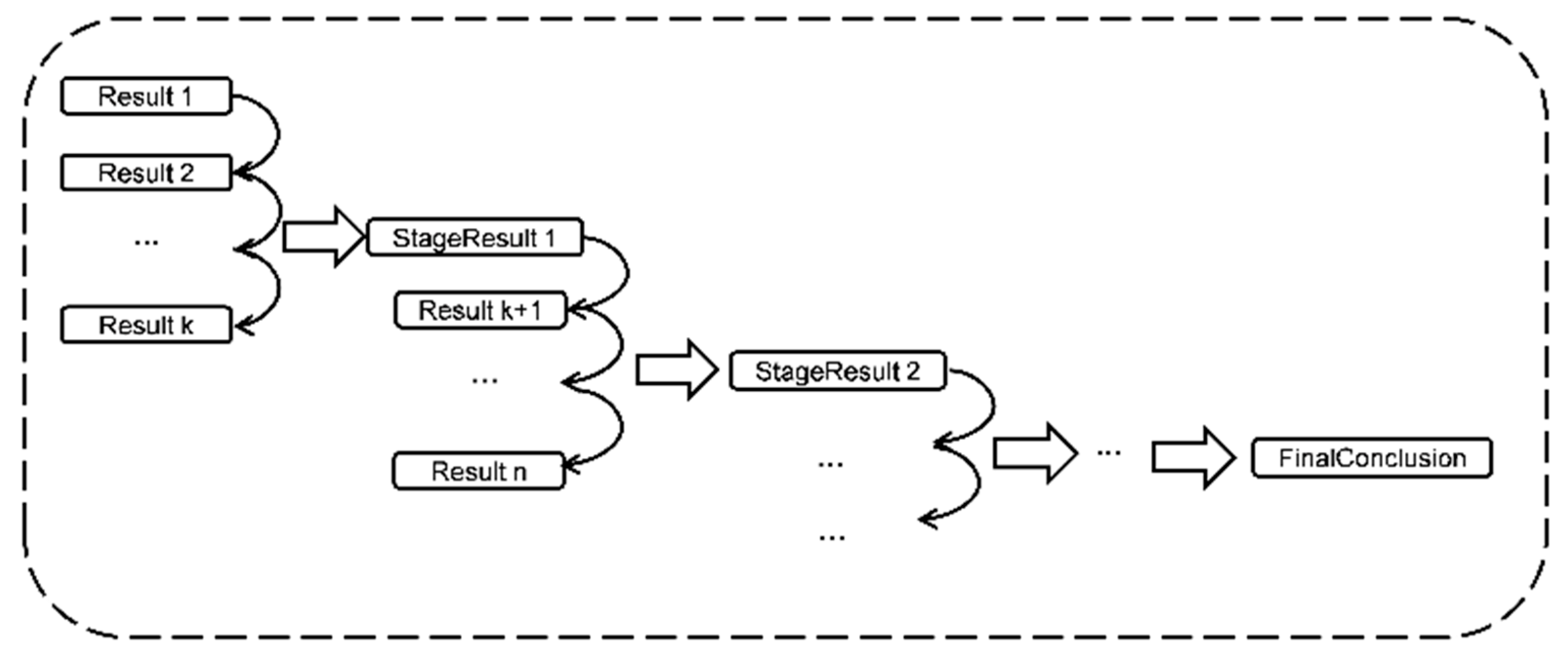
3.3. Results Statistics

The test data enters each test model, and the relevant results obtained in each round are recorded after the test: (1) probability Pi for each category, (2) probability ranking for each category Ri, (3) number of model N, and (4) the number of categories K to which the test data may belong. The statistics obtained the (2), (3), and (4) portions, using (5) to calculate a weighted average function, to give the corresponding probability P, defined as follows:$F(P_i,R_i,N,K)$.

(1) Judging the probability $P_i$ belonging to each category:

$${\displaystyle \sum _{i=1}^k}{P}_i=1$$

(3)

(2) Judging the probability ranking $R_i$ belonging to each category:

$$R_i\in [1,k]$$

(4)

(3) Number of models N:

The number of models represents the number of all models that have passed, and the data of the $N$ sets of results are used to count the final weighted average.

(4) Number of categories K:

$K$ is the number of categories in the classification.

(5) A weighted average function $F(P_i,R_i,N,K)$:

$$F(P_i,R_i,N,K)=G(R_i,N,k)\ast \frac{{\displaystyle {\sum }_{i=1}^N{P}_i}}{N}$$

(5)

$G\left(R_{{}_i},N\right)$ is defined as follows:

$$G\left(R_i,N,K\right)=\frac{{\displaystyle {\sum }_{i=1}^N(K-P_i+1)}}{N\ast K}$$

(6)

$K$ represents the number of all data categories.

$F(P_i,R_i,N,K)$ represents the set of test results, the probability that the test data belongs to each final category.

$G(R_i,N,K)$ represents the weight of the average probability reliability in the $N$ test results, and:

$${\displaystyle \sum _{i=1}^K(P_i,R_i,N,K)\le 1}$$

(7)

In the end, it is only necessary to compare the $F(P_i,R_i,N,K)$ values of the test data pair divided into a certain class, and then, a definitive division conclusion can be obtained.

3.4. Model Update Strategy

The model update strategy is shown in Figure 3. The update strategy starts in turn at the beginning of each model test.

Figure 3. The strategy of the model update.

After passing the Kth model, the K models are compared, and the test data is identified as the probability of each class and the corresponding probability ranking. The group with the worst results will be automatically rejected. Use the weighted average function in Section 3.3 to obtain the result data of the first stage, and use this data as the initial result data of the second stage. Repeat the above process until all the model test results have been processed, and you can get the final recognition conclusion, which is FinalConclusion. Each stage includes S group data—that is, after each S group data is passed, a model update is performed. S is a manually set hyperparameter.

The significance of this strategy is that, because less data is trained for each model, the stability and accuracy of the model need to be given more attention. Adding this strategy to the framework by longitudinally comparing the test results between different models and screening and removing the less effective results can achieve the purpose of maintaining the model stability and improving the conclusion accuracy.

4. Experiment

4.1. Data Preparation

The flowers dataset from TensorFlow [9] and the car dataset from ImageNet [10] were used as the experimental set. The flowers dataset includes daisy, sunflowers, roses, tulips, and dandelions (five). The training part selected the format of 10 * 5 * 21—that is, a total of 10 sets of training data were used to generate 10 different image classifiers. Each of the five flowers described above contains 21 pictures to meet the minimum requirements for the training pictures. The car dataset includes SUV, trucks, sportscars, and sedans. The training part selects the 10 * 4 * 21 format. The explanation is the same as above.

In the corresponding test set, the test data and training data are from the same source. The format of the flowers part test data is 2 * 5—that is, there are 2two images in each of the five types of flowers. The car part is 2 * 4.

The two sets of experimental data ensure that the pictures of each group (both in JPG format) are different from each other, which is conducive to suppressing overfitting and makes the generalized ability of the trained image classifier better.

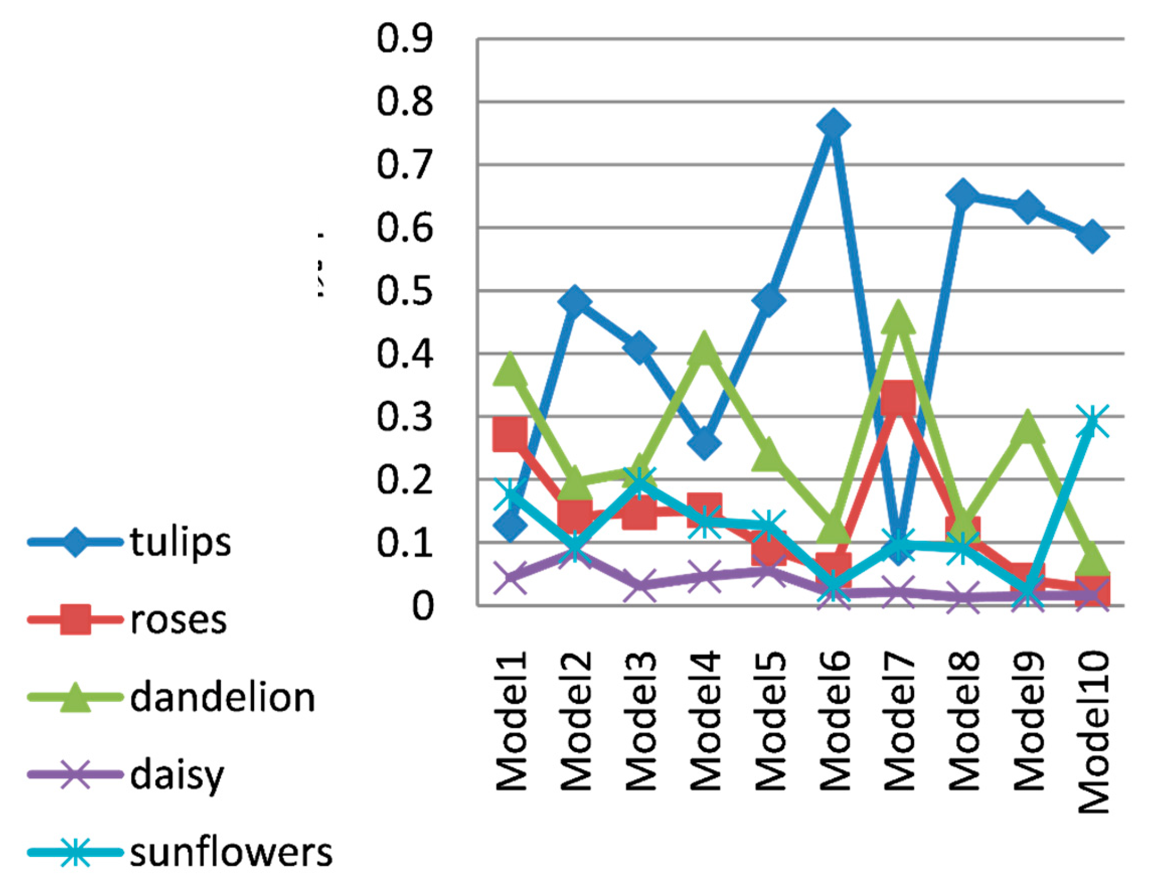
4.2. Training and Statistical Results

4.2.1. Flowers Dataset

The prepared 10 flowers dataset was input into the image classifier file in the TensorFlow platform in batches. After training, 10 different models were obtained (each model includes two files with extensions.pb and .txt, respectively), labeled $Mode{l}_i,i\in [1,10]$.These 10 models are used to simulate the training model obtained after data input in 10 stages in the real-time system.

Pass the 10 test set pictures of the prepared flowers through 10 models and record them in different models, corresponding to the probability $P_i$ that belongs to a certain flower type and the corresponding ranking $R_i$.

Due to the large amount of data obtained after the test, only the results after the TulipsTest1 test in the test data are shown in Figure 4.

Figure 4. Results after the TulipsTest1 test in the test data.

It can be seen that the recognition effect of the 10 models obtained from training with a small amount of data is not good. In many models, the probability of correct classification is not the first and even falls to the fourth. This clearly shows that, in real-time systems, the use of deep-learning methods is not effective due to the small amount of data.

Count the probability rankings belonging to different categories in each model; the probability rankings belonging to different categories in each model are shown in Table 1.

Table 1. Table shows the probability rankings belonging to different categories in each model.

Model	Tulips	Roses	Daisy	Dandelion	Sunflower
1	4	3	1	2	5
2	1	3	5	2	4
3	1	4	5	2	3
4	2	3	5	1	4
5	1	4	5	2	3
6	1	3	5	2	4
7	4	2	5	1	3
8	1	3	5	2	4
9	1	3	4	2	5
10	1	4	5	3	2

Use the weighting function $F(P_i,R_i,N,K)$ in Section 3.3 to calculate the above data. Taking the identification as tulips as an example, calculate as follows:

(1) Average probability of recognition as tulips:

$$\stackrel{-}{P}=\frac{{\displaystyle {\sum }_{i=1}^N{P}_i}}{N}$$

(8)

Calculated $\stackrel{-}{P}=0.448828$.

(2) Corresponding weights identified as tulips:

$$G(R_i,N,K)=\frac{{\displaystyle {\sum }_{i=1}^N(K-P_i+1)}}{N\ast K},K=5$$

(9)

Calculated $G(R_i,N,K)=0.86$.

(3) Probability that it is considered to belong to the tulips after calculation:

Calculated $F(P_i,R_i,N,K)=0.385992$.

(4) Conclusions obtained after calculating the probability of flowers belonging to the remaining four categories; the probability of flowers belonging to the remaining four categories are shown in Table 2.

Table 2. The probability of flowers belonging to the remaining four categories.

Model	Tulips	Roses	Daisy	Dandelion	Sunflower
Probability	0.386	0.080	0.011	0.206	0.066

Compared with the probability of being recognized as tulips, it can be seen that the probability of being recognized as tulips is far greater than the probability of being recognized for the remaining four categories. At this time, the system can assert that the test picture belongs to tulips. Compared with the real label tulips, it is also consistent.

(5) When applying the model update strategy:

Assume that every three batches of conclusions are screened and rejected; as described above, five sets of data are calculated and compared with the previous results. Every three batches of conclusions are shown in Table 3.

Table 3. Table shows every three batches of conclusions.

Batch	Model	Probability	Rank	Whether to Eliminate (Y/N)
1	Model 1	0.128	4	Y
1	Model 2	0.483	1	N
1	Model 3	0.410	1	N
2	Stage1	0.446	1	N
2	Model 4	0.258	2	Y
2	Model 5	0.485	1	N
3	Stage2	0.457	1	N
3	Model 6	0.763	1	N
3	Model 7	0.091	4	Y
4	Stage3	0.614	1	N
4	Model 8	0.652	1	N
4	Model 9	0.633	1	N
5	Stage4	0.642	1	N
5	Model 10	0.586	1	Y

After using the model update strategy, we can see that, for the correct identification of classifications, the probability on tulips has been further greatly improved, reaching 0.642649, far exceeding 0.385992 without using the model update strategy before. The probability of misclassification has also been further reduced. Therefore, it can be asserted that the test picture is tulips, which conforms to its label. The model update strategy is used to further improve the recognition accuracy and stability of the system.

4.2.2. Cars Dataset

The same method was used to verify the effectiveness of the framework for the car dataset. Taking SedanTest1 as an example, the probability after passing the framework is shown in Table 4.

Table 4. Comparison with the previous results.

Type	Before	After
Tulip	0.385992	0.643649
Rose	0.206354	0.142315
Daisy	0.065914	0.010431
Dandelion	0.010578	0.005371
Sunflower	0.079717	0.029415

It can be seen that the system’s correct recognition result is also ranked first when the dataset is replaced without adding a model update strategy, but it is not much different from the second incorrect recognition result. However, after adding the model update strategy, the probability of correct recognition is greatly improved.

5. Conclusions

As mentioned in the introduction, currently, although deep learning has greatly helped many fields such as pattern recognition, computer vision, natural language processing, etc., its further development is greatly restricted due to the limited amount of data. Previous scholars and literature [11] used reasonable mathematical methods to process the results to obtain better results. This framework is suitable for real-time classification and the analysis of small batches of data in real-time systems for classification. It adopts a statistical method for processing the results and achieves good results but still has great limitations and deficiencies. In addition to this article, there have been related scholars who have completed the evaluation under the framework of neural networks by using probability and statistics methods. The artificial intelligence represented by current deep learning has problems, such as the incomplete simulation of human brain functions. We hope that, through the use of mathematical statistics on the results, we will initially solve some of the shortcomings in deep learning in terms of small amounts of data and the simulation of human cognitive methods, which will cause scholars and the industry to think.

References

1. Krizhevsky, A.; Sutskever, I.; Hinton, G.E. Imagenet classification with deep convolutional neural networks. Adv. Neural Inf. Proc. Syst. 2012, 60, 1097–1105. [Google Scholar] [CrossRef]
2. Hinton, G.E.; Osindero, S.; Teh, Y.W. A fast learning algorithm for deep belief nets. Neural Comput. 2006, 18, 1527–1554. [Google Scholar] [CrossRef] [PubMed]
3. Simard, P.Y.; Steinkraus, D.; Platt, J.C. Best practices for convolutional neural networks applied to visual document analysis. ICDAR 2003, 3, 958–962. [Google Scholar]
4. Neumaier, A. Solving ill-conditioned and singular linear systems: A tutorial on regularization. SIAM Rev. 1998, 40, 636–666. [Google Scholar] [CrossRef]
5. Srivastava, N.; Hinton, G.; Krizhevsky, A.; Sutskever, I.; Salakhutdinov, R. Dropout: A simple way to prevent neural networks from overfitting. J. Mach. Learn. Res. 2014, 15, 1929–1958. [Google Scholar]
6. Guo, K.; Duan, G. 3D image retrieval based on differential geometry and co-occurrence matrix. Neural Comput. Appl. 2014, 24, 715–721. [Google Scholar] [CrossRef]
7. Szegedy, C.; Vanhoucke, V.; Ioffe, S.; Shlens, J.; Wojna, Z. Rethinking the inception architecture for computer vision. In Proceedings of the IEEE Conference on Computer Vision and Pattern Recognition, Las Vegas, NV, USA, 27–30 June 2016; pp. 2818–2826. [Google Scholar]
8. Guo, K.; Xiao, Y.; Duan, G. A cost-efficient architecture for the campus information system based on transparent computing platform. Int. J. Ad Hoc Ubiquitous Comput. 2016, 21, 95–103. [Google Scholar] [CrossRef]
9. Guo, K.; Liu, Y.; Duan, G. Differential and statistical approach to partial model matching. Math. Probl. Eng. 2013. [Google Scholar] [CrossRef]
10. Zhu, Y.; Sun, D.; He, X.; Liu, M. Short-term wind speed prediction based on EMD-GRNN and probability statistics. Comput. Sci. 2014, 41, 72–75. [Google Scholar]
11. Liu, D.; Li, S.; Cao, Z. A Review of deep learning and its application in image object classification and detection. Comput. Sci. 2016, 43, 13–23. [Google Scholar]
Article Metrics
Citations
Article Access Statistics
Multiple requests from the same IP address are counted as one view.