Machine Learning-Based Prediction of a BOS Reactor Performance from Operating Parameters

Abstract
1. Introduction
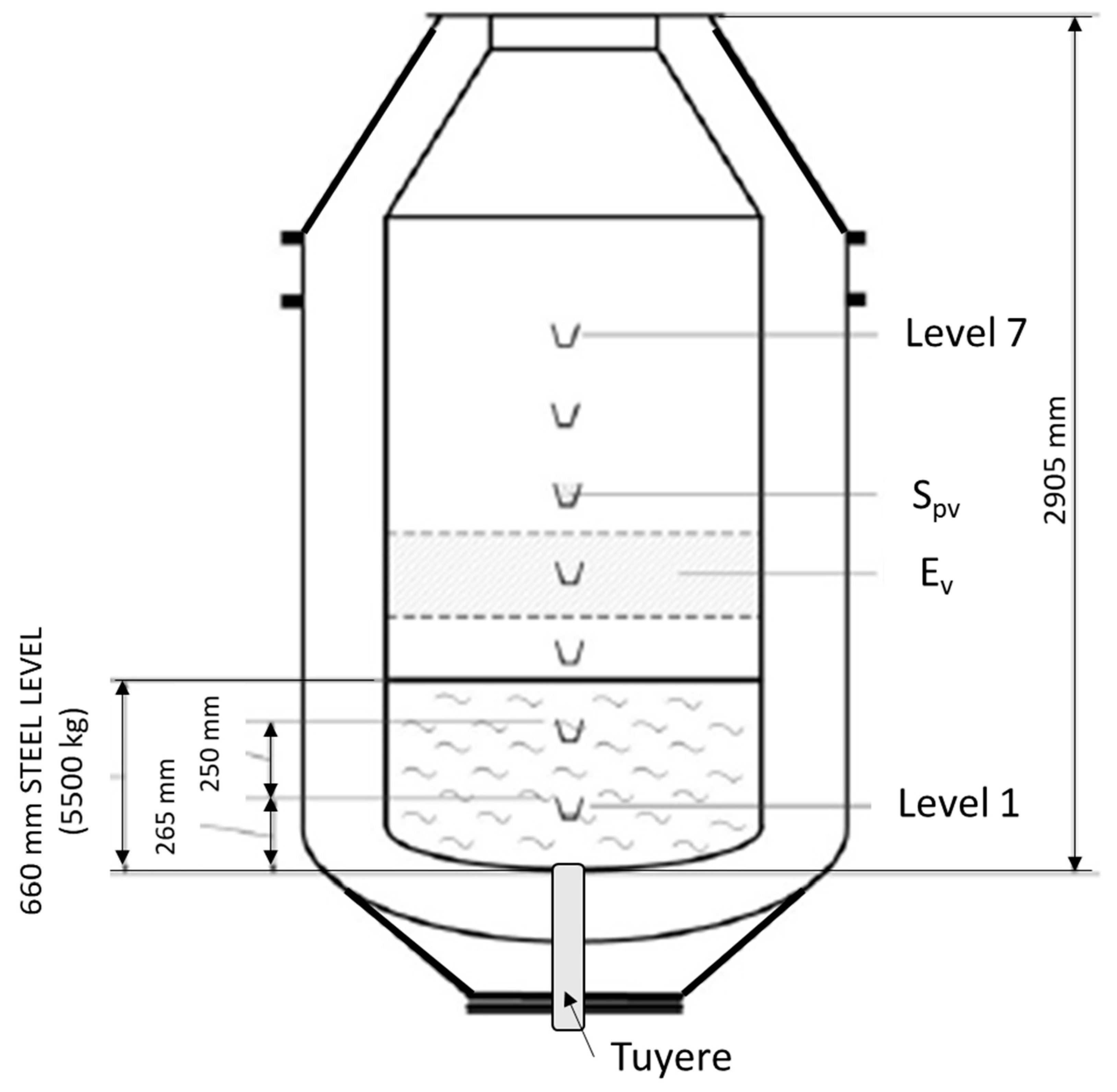
2. The Multiphysics of the Basic Oxygen Steelmaking Process
3. Dataset
4. Method
5. Results and Discussion
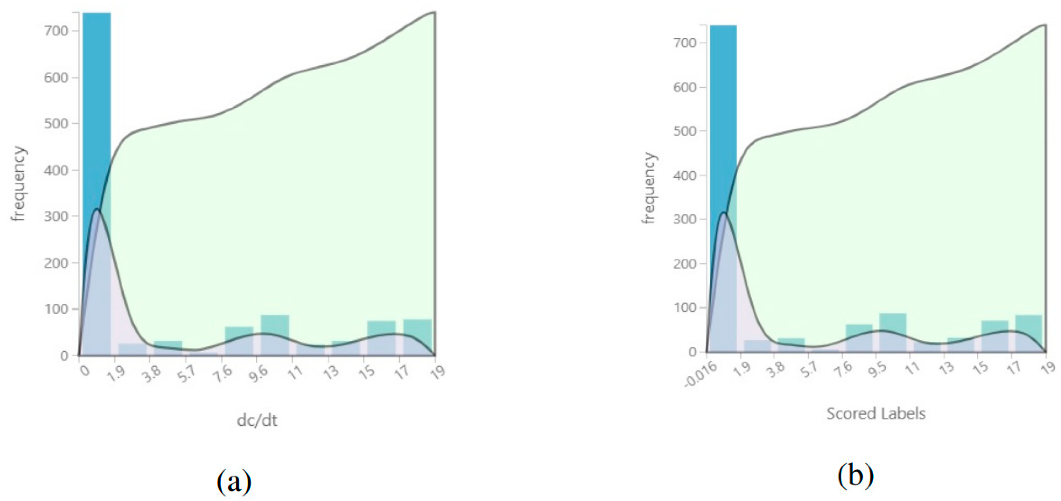
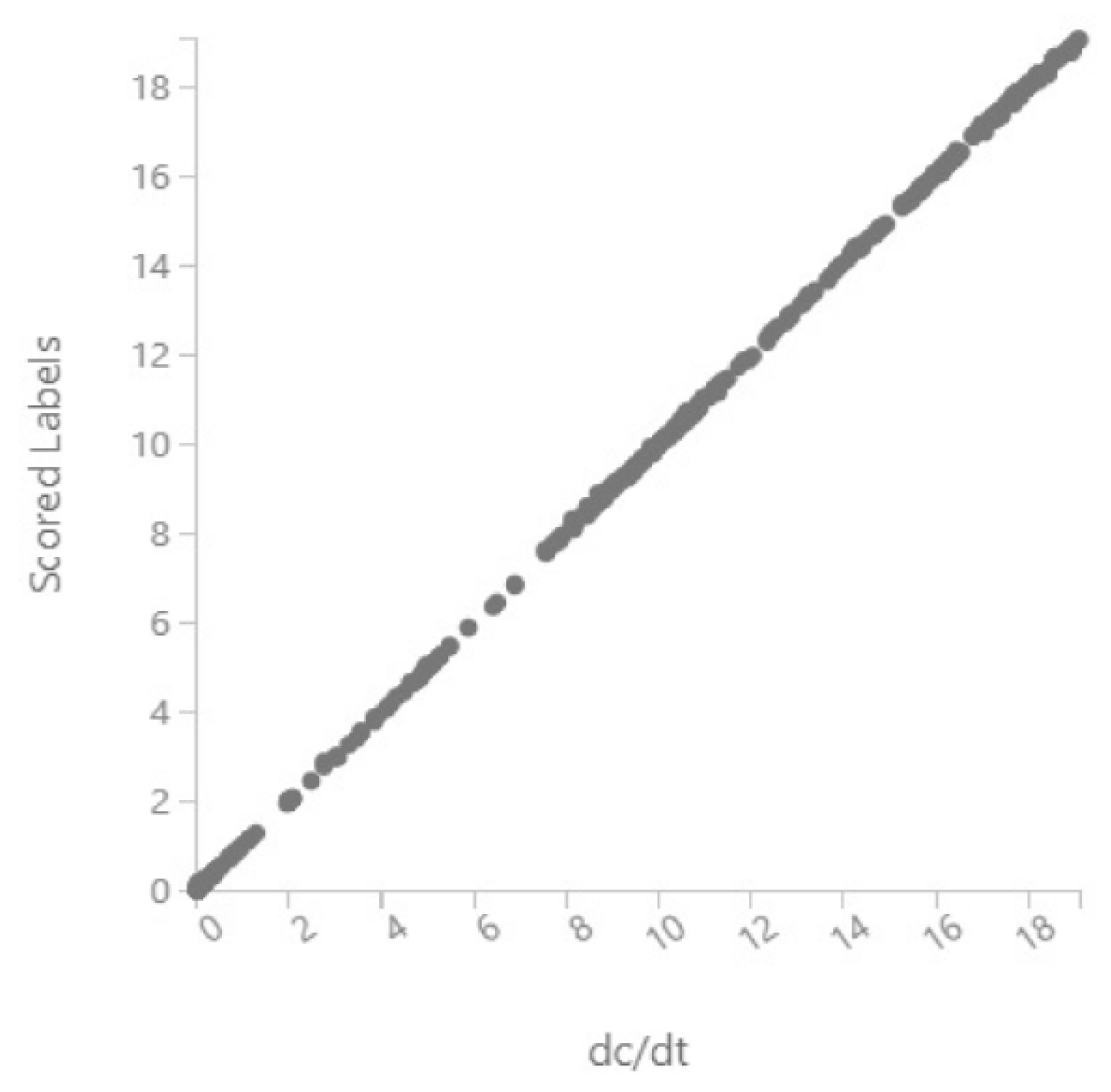
5.1. Machine Learning Predictions of the Decarburization Rate dc/dt
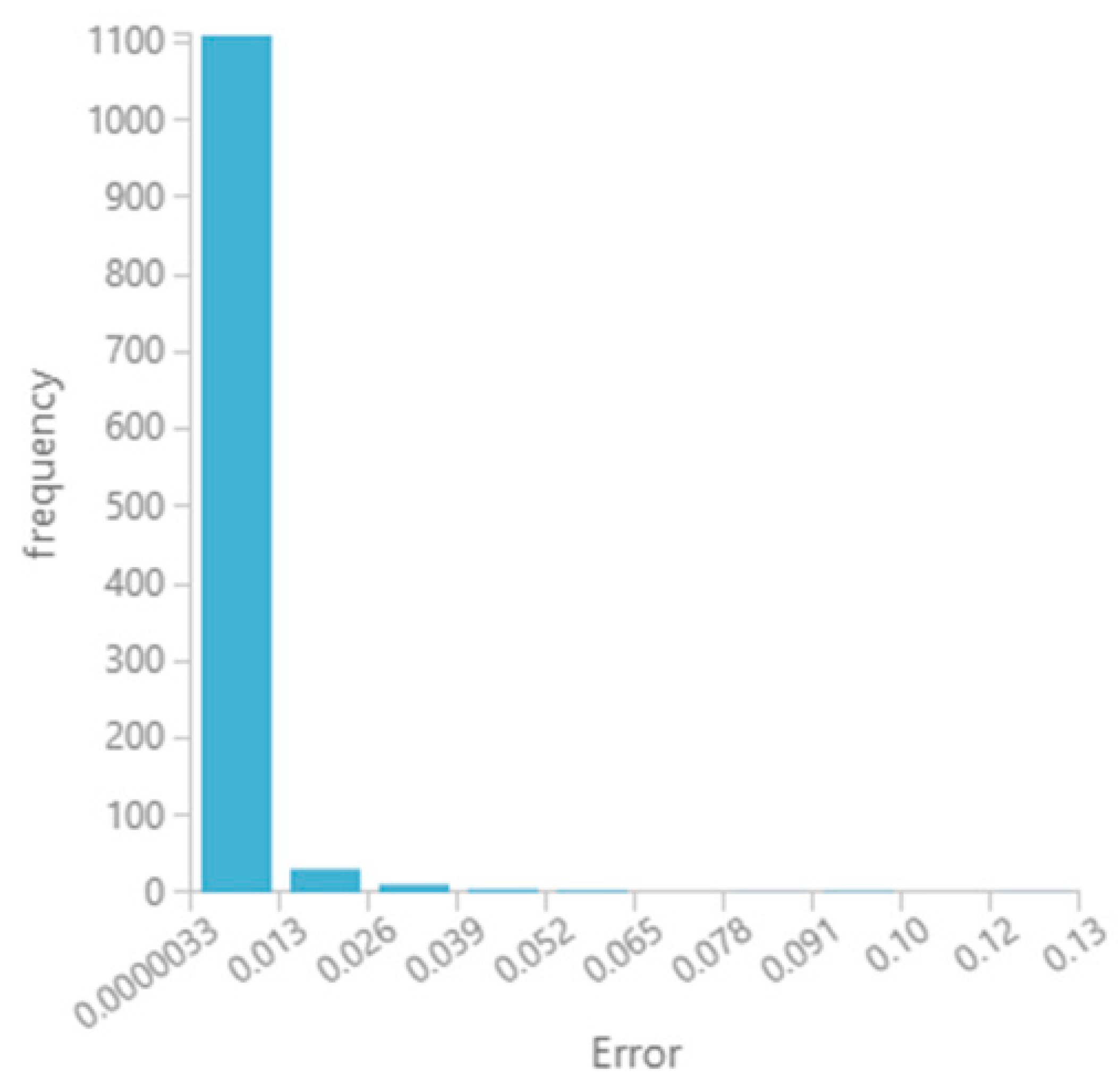
5.2. Prediction of dc/dt With All the Features Included in the Dataset
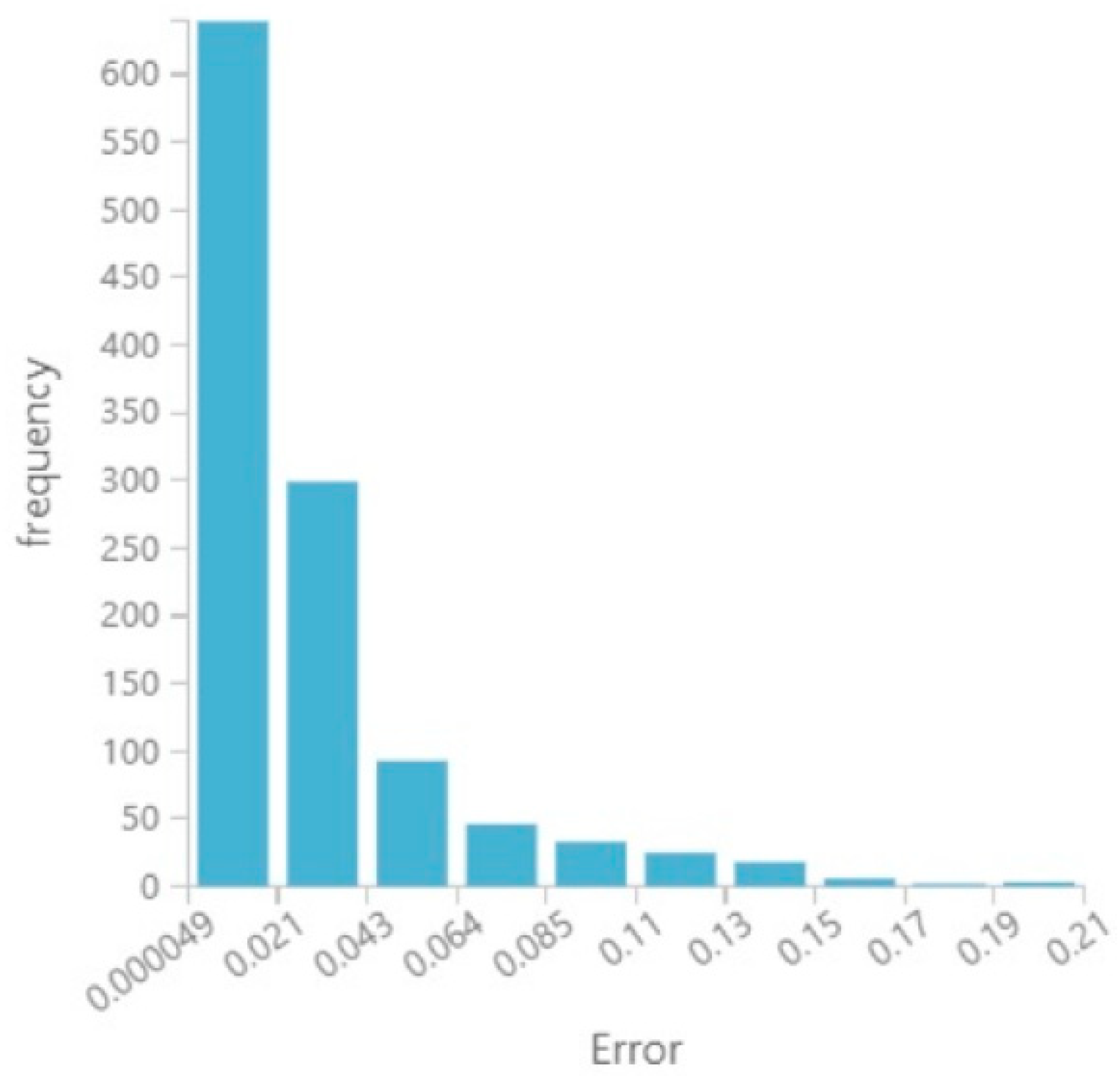
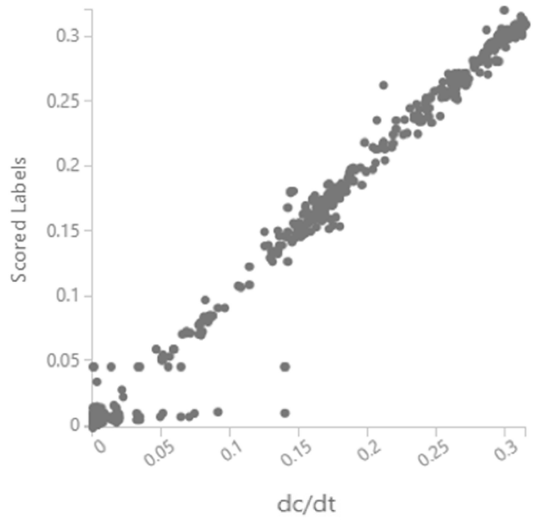
5.3. Prediction of the dc/dt After Excluding Parameters
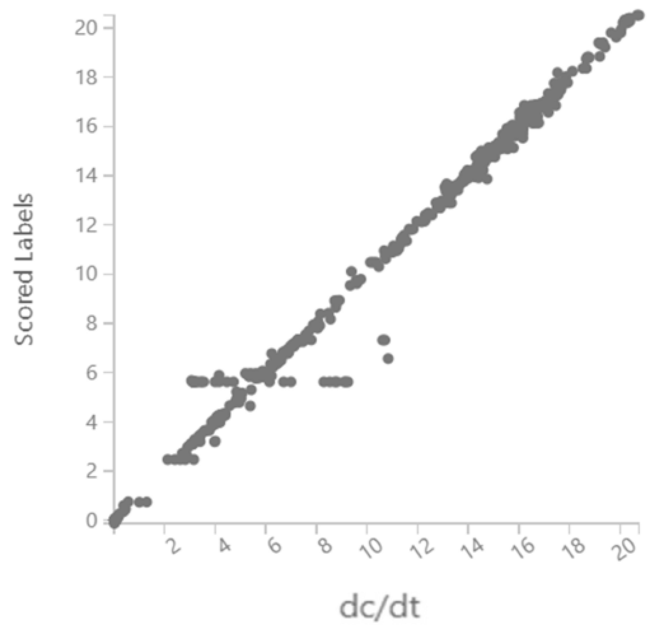
5.4. Prediction of the dc/dt for an Industrial Dataset
6. Conclusions
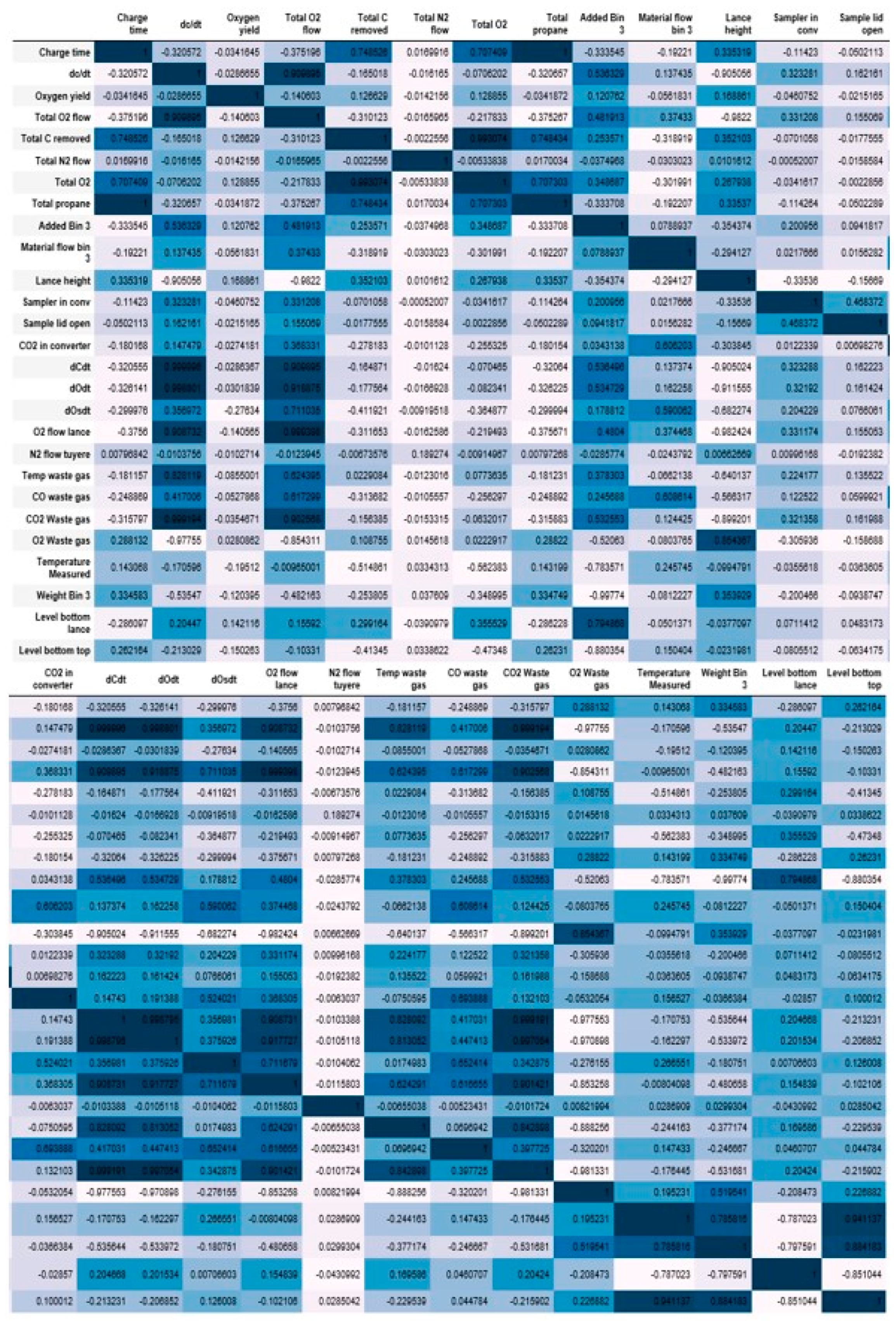
- A strong positive correlation between the rate of decarburization (dc/dt) and total oxygen flow.
- A negative correlation with lance height.
- Less obviously, the decarburization also showed a positive correlation with the temperature of the waste gas, CO2 content in the waste gas and O2 in the waste gas.
- The pilot plant dataset was used for training and test data to develop a neural network-based regression to predict the decarburization rate. The developed algorithm was used successfully to predict the decarburization rate in a BOS furnace in an actual manufacturing plant based on the two operating parameters of total oxygen flow and lance height only.
- The performance was satisfactory, with a coefficient of determination of 0.98, confirming that the trained model can adequately predict the variation in the dc/dt within BOS reactors.
Author Contributions
Funding
Acknowledgments
Conflicts of Interest
References
- Ogawa, Y.; Yano, M.; Kitamura, S.; Hirata, H. Development of the continuous dephosphorization and decarburization process using BOF. Steel Res. Int. 2003, 74, 70–76. [Google Scholar] [CrossRef]
- Millman, M.S.; Kapilashrami, A.; Bramming, M.; Malmberg, D. IMPHOS—Improving Phosphorus Refining; European Commission, Research Fund for Coal and Steel: Luxembourg, 2011; ISSN 1831-9424. [Google Scholar]
- Jung, I.H.; Hudon, P.; Van Ende, M.A.; Kim, W.Y. Thermodynamic database for P2O5-containing slags and its application to the dephosphorization process. In Proceedings of the Iron & Steel Technology Conference, Indianapolis, IN, USA, 5–8 May 2014; Volume 1, pp. 1257–1268. [Google Scholar]
- Rout, B.; Brooks, G.; Rhamdhani, M.A.; Li, Z.; Schrama, F.N.; Sun, J. Dynamic model of basic oxygen steelmaking process based on multi-zone reaction kinetics: Model derivation and validation. Metall. Mater. Trans. B 2018, 49, 537–557. [Google Scholar] [CrossRef]
- Ersson, M.; Hoglund, L.; Tilliander, A. Dynamic coupling of computational fluid dynamics and thermodynamics software: Applied on a top blown converter. ISIJ Int. 2008, 48, 147–153. [Google Scholar] [CrossRef]
- Cox, I.J.; Lewis, R.W.; Ransing, R.S. Application of neural computing in basic oxygen steelmaking. J. Mater. Process. Technol. 2002, 120, 310–315. [Google Scholar] [CrossRef]
- Das, A.; Maiti, J.; Banerjee, R.N. Process control strategies for a steelmaking furnace using ann with Bayesian regularization and anfis. Expert Syst. Appl. 2010, 37, 1075–1085. [Google Scholar] [CrossRef]
- Han, M.; Zhao, Y. Dynamic control model of BOF steelmaking process based on anfis and robust relevance vector machine. Expert Syst. Appl. 2011, 38, 14786–14798. [Google Scholar] [CrossRef]
- Kubat, C.; Takin, H.; Artir, R.; Yilmaz, A. Bofy-fuzzy logic control for the basic oxygen furnace. Robot. Auton. Syst. 2004, 49, 193–205. [Google Scholar] [CrossRef]
- Wang, X.; Han, M.; Wang, J. Applying input variables selection technique on input weighted support vector machine modeling for BOF end point prediction. Eng. Appl. Artif. Intell. 2010, 23, 1012–1028. [Google Scholar] [CrossRef]
- Xu, L. A model of basic oxygen furnace (BOF) endpoint prediction based on spectrum information of the furnace flame with support vector machine (SVM). Optik 2011, 122, 594–598. [Google Scholar] [CrossRef]
- Wang, X.; Xing, J.; Dong, J.; Wang, Z. Data driven based endpoint carbon content real time prediction for BOF steelmaking. In Proceedings of the 36th Chinese Control Conference (CCC), Dalian, China, 26–28 July 2017; pp. 9708–9713. [Google Scholar]
- Liu, Y.; Zhao, T.; Ju, W.; Shi, S. Materials discovery and design using machine learning. J. Mater. 2017, 3, 159–177. [Google Scholar] [CrossRef]
- Ward, L.; OKeeffe, S.C.; Stevick, J.; Jelbert, G.R.; Aykol, M.; Wolverton, C. A machine learning approach for engineering bulk metallic glass alloys. Acta Mater. 2018, 159, 102–111. [Google Scholar] [CrossRef]
- Li, W.; Jacobs, R.; Morgan, D. Predicting the thermodynamic stability of perovskite oxides using machine learning models. Comput. Mater. Sci. 2018, 150, 454–463. [Google Scholar] [CrossRef]
- Cassar, D.R.; de Carvalho, A.C.; Zanotto, E.D. Predicting glass transition temperatures using neural networks. Acta Mater. 2018, 159, 249–256. [Google Scholar] [CrossRef]
- Meredig, B.; Agrawal, A.; Kirklin, S.; Saal, J.E.; Doak, J.W.; Thompson, A.; Zhang, K.; Choudhary, A.; Wolverton, C. Combinatorial screening for new materials in unconstrained composition space with machine learning. Phys. Rev. B 2014, 89, 094104. [Google Scholar] [CrossRef]
- Rahnama, A.; Clark, S.; Sridhar, S. Machine learning for predicting occurrence of interphase precipitation in HSLA steels. Comput. Mater. Sci. 2018, 154, 169–177. [Google Scholar] [CrossRef]
- Ramprasad, R.; Batra, R.; Pilania, G.; Mannodi-Kanakkithodi, A.; Kim, C. Machine learning in materials informatics: Recent applications and prospects. Npj Comput. Mater. 2017, 3, 1–13. [Google Scholar] [CrossRef]
- Available online: https://docs.microsoft.com/en-us/azure/machine-learning/studio-module-reference/multiclass-neural-network (accessed on 2 January 2020).
- Chattopadhyay, K.; Isac, M.; Guthrie, R.I.L. Applications of Computational Fluid Dynamics (CFD) in iron- and steelmaking (part I & part II). Ironmak. Steelmak. 2010, 37, 554–569. [Google Scholar]
- Ek, M.; Shu, Q.F.; van Boggelen, J.; Sichen, D. New approach towards dynamic modelling of dephosphorisation in converter process. Ironmak. Steelmak. 2012, 39, 77–84. [Google Scholar] [CrossRef]
- Oguchi, S.; Robertson, D.G.C.; Deo, B.; Grieveson, P.; Jeffes, J.H.E. Simultaneous dephosphorization and desulphurization of molten pig iron. Ironmak. Steelmak. 1984, 11, 202–213. [Google Scholar]
- Spooner, S.; Rahnama, A.; Warnett, J.M.; Williams, M.A.; Li, Z.; Sridhar, S. Quantifying the Pathway and Predicting Spontaneous Emulsification during Material Exchange in a Two Phase Liquid System. Sci. Rep. 2017, 7, 14384. [Google Scholar] [CrossRef]
- Spooner, S.; Li, Z.; Sridhar, S. Spontaneous emulsification as a function of material exchange. Sci. Rep. 2017, 7, 5450. [Google Scholar] [CrossRef] [PubMed]
- Dogan, N.; Brooks, G.A.; Rhamdhani, M.A. Kinetics of decarburization reaction in oxygen steelmaking process. In High Temperature Processing Symposium; Swinburne University of Technology: Melbourne, Australia, 2010; pp. 9–11. [Google Scholar]
- The AISE Steel Foundation. The Making, Shaping and Treating of Steel (Steelmaking and Refining Volume); AIST: Pittsburgh, PA, USA, 1998; pp. 475–524. [Google Scholar]


| Parameter | Feature |
|---|---|
| Charge Time (min) | Blowing time (in minutes from O2 ignition) |
| dc/dt (kg C/min) | Instant decarburization rate |
| Oxygen Yield (%) | Instant oxygen yield |
| Total Oxygen flow rate (Nm3/min) | Instant oxygen flow rate |
| Total C removal (kg) | Calculated total C removed from the start of O2 |
| Total N2 flow rate (Nm3/min) | Instant N2 flow rate |
| Total O2 (Nm3/min) | Total blown oxygen volume |
| Total N2 (Nm3/min) | Total bottom blown nitrogen volume |
| Total propane (Nm3/min) | Total blown propane volume |
| Lance height (mm) | Instant lance height from the point of calculated metal bath level |
| dC/dt (kg C/s) | Calculated from off-gas composition |
| dO/dt (kg O/s) | Calculated from off-gas, oxygen for decarburization |
| dOs/dt (kg O/s) | Calculated from off-gas composition, oxygen into slag |
| Temp. waste gas (°C) | Off-gas temperature (measured after water cooling) |
| CO waste gas (%) | Measured waste gas composition |
| CO2 waste gas (%) | Measured waste gas composition |
| O2 waste gas (%) | Measured waste gas composition |
| 6t pilot BOF. | C | Si | Mn | P | S | T (֯C) | |
|---|---|---|---|---|---|---|---|
| Hot metal (%) | 3.78~4.25 | 0.41~0.88 | 0.39~0.48 | 0.067~0.095 | 0.037~0.081 | 1272~1316 | |
| Steel (%) | 0.01~0.41 | 0~0.15 | 0.05~0.27 | 0.008~0.042 | 0.018~0.035 | 1669~1772 | |
| CaO | SiO2 | FeO | MnO | Al2O3 | MgO | P2O5 | |
| Slag (%) | 26.2~52.3 | 6.7~19.2 | 8.3~30.5 | 2.6~4.1 | 0.7~1.6 | 4.6~17.7 | 0.73~1.62 |
| 330t BOF | C | Si | Mn | P | S | T (℃) | |
| Hot metal (%) | 3.60~5.18 | 0.30~1.20 | 0.11~0.52 | 0.058~0.125 | 0.025~0.072 | 1341~1412 | |
| Steel (%) | 0.021~0.55 | 0~0.10 | 0.03~0.21 | 0.001~0.057 | 0.011~0.032 | 1579~1738 | |
| CaO | SiO2 | FeO | MnO | Al2O3 | MgO | P2O5 | |
| Slag (%) | 36.07~55.35 | 9.13~19.58 | 12.15~31.34 | 2.04~5.62 | 0.64~4.97 | 3.61~10.73 | 0.94~2.38 |
| 6t pilot BOF | 330t BOF | ||||||
| hot metal | 4410~5170 kg | 269.6~302.5 t | |||||
| scrap | 500~750 kg | 46.0~85.5 t | |||||
| lime | 250~350 kg | 5~25 t | |||||
| dolomet | 0~30 kg | 0~11.5 t | |||||
| iron ore | 0 kg | 0~6.5 t | |||||
| total oxygen | 263~307 Nm3 | 12265~21641 Nm3 | |||||
| Lance height | 110~180 mm | 2.0~2.6 m | |||||
| Evaluated Metrics | Pilot Dataset with All Features (1) | Pilot Dataset with All Features (2) | Pilot Dataset without dc/dt (2) | Pilot Dataset with Total O2 Flow and Lance Height Only (2) | Industrial Dataset with Total O2 Flow and Lance Height Only (2) |
|---|---|---|---|---|---|
| Mean Absolute Error | 0.12 | 0.029 | 0.030 | 0.034 | 0.25 |
| Root Mean Square Error | 0.51 | 0.043 | 0.055 | 0.060 | 0.62 |
| Relative Absolute Error | 0.42 | 0.005 | 0.006 | 0.008 | 0.04 |
| Relative Square Error | 0.48 | 0.000046 | 0.00006 | 0.0001 | 0.009 |
| Coefficient of Determination | 0.45 | 0.99 | 0.99 | 0.97 | 0.98 |
| Mean | Median | Min | Max | Standard Deviation | |
|---|---|---|---|---|---|
| Actual Statistics | 4.43 | 0.081 | 0 | 19.105 | 6.42 |
| Predicted Statistics | 4.45 | 0.092 | 0 | 19.09 | 6.43 |
| dC/dt | dO/dt | Oxygen Yield | CO2 Waste Gas | CO Waste Gas | Total O2 Flow | dOs/dt | Temp. of Waste Gas | Total O2 | O2 Waste Gas |
|---|---|---|---|---|---|---|---|---|---|
| 9.06 | 0.16 | 0.07 | 0.04 | 0.004 | 0.002 | 0.0006 | 0.0002 | 0.00014 | 0.00013 |
© 2020 by the authors. Licensee MDPI, Basel, Switzerland. This article is an open access article distributed under the terms and conditions of the Creative Commons Attribution (CC BY) license (http://creativecommons.org/licenses/by/4.0/).
Share and Cite
Rahnama, A.; Li, Z.; Sridhar, S. Machine Learning-Based Prediction of a BOS Reactor Performance from Operating Parameters. Processes 2020, 8, 371. https://doi.org/10.3390/pr8030371
Rahnama A, Li Z, Sridhar S. Machine Learning-Based Prediction of a BOS Reactor Performance from Operating Parameters. Processes. 2020; 8(3):371. https://doi.org/10.3390/pr8030371
Chicago/Turabian StyleRahnama, Alireza, Zushu Li, and Seetharaman Sridhar. 2020. "Machine Learning-Based Prediction of a BOS Reactor Performance from Operating Parameters" Processes 8, no. 3: 371. https://doi.org/10.3390/pr8030371
APA StyleRahnama, A., Li, Z., & Sridhar, S. (2020). Machine Learning-Based Prediction of a BOS Reactor Performance from Operating Parameters. Processes, 8(3), 371. https://doi.org/10.3390/pr8030371