Steel Wool for Water Treatment: Intrinsic Reactivity and Defluoridation Efficiency

 , ,
, , 
Abstract
1. Introduction
2. Material and Methods
2.1. Aqueous Solutions
2.1.1. EDTA
2.1.2. TISAB
2.1.3. Methylene Blue (C16H18CIN3S)
2.1.4. Additional Solutions
2.2. Solid Materials
2.2.1. Sand
2.2.2. Steel Wool (Fe0)
2.3. Experimental Procedure
2.3.1. Iron Dissolution in EDTA
Batch Experiments
Column Experiments
2.3.2. Methylene Blue (MB) Discoloration
2.3.3. Fluoride Removal
Batch Experiments
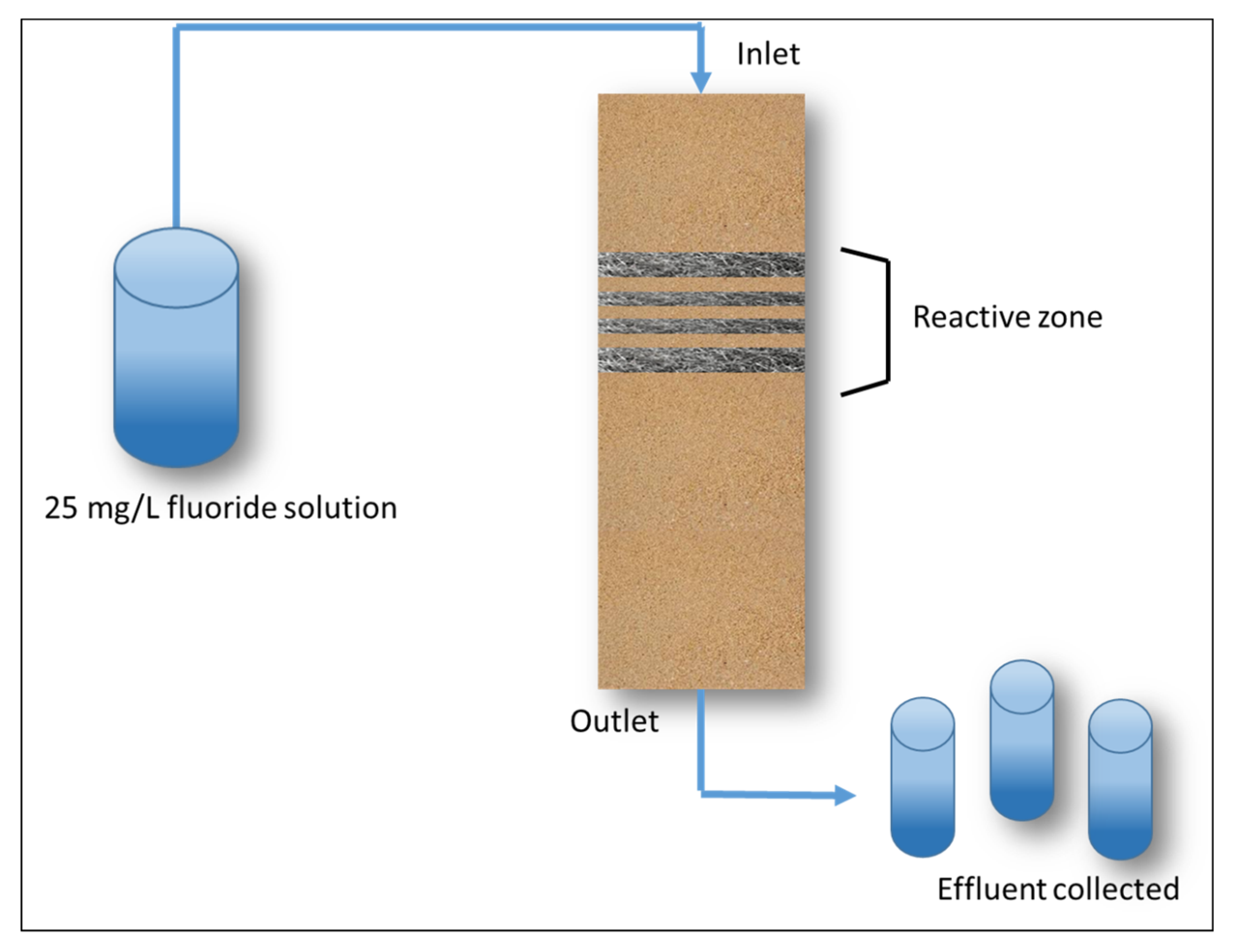
Column Experiments
2.4. Analytical Methods
2.4.1. UV-Vis Spectrophotometry
2.4.2. pH Meter
2.4.3. Fluoride Electrode
2.5. Expression of Experimental Results
2.5.1. Kinetics of Fe0 Oxidative Dissolution (kEDTA Value)
2.5.2. Removal Efficiency (E Value)
3. Results and Discussion
3.1. Iron Dissolution in EDTA
3.1.1. Appropriateness of the Experimental Approach
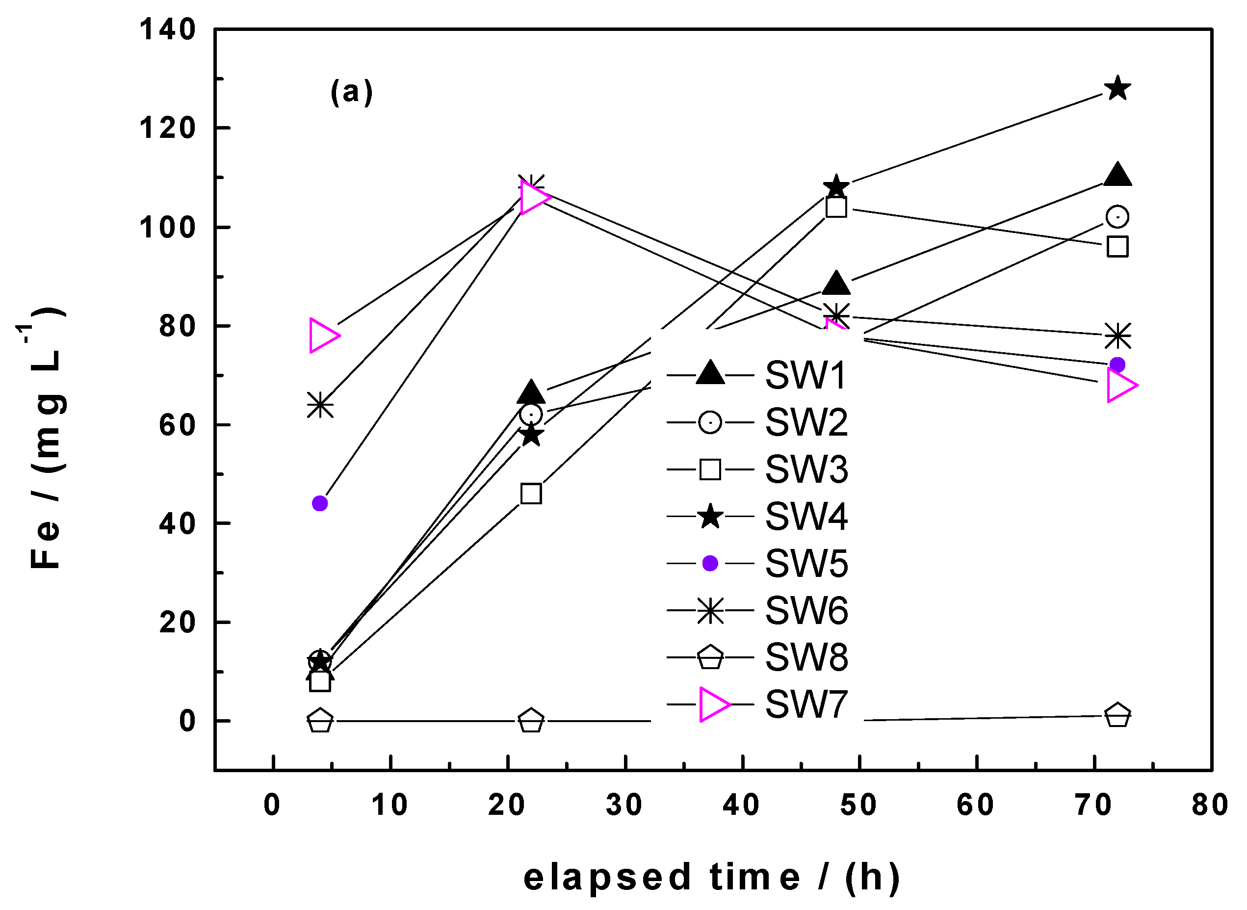
3.1.2. kEDTA Values
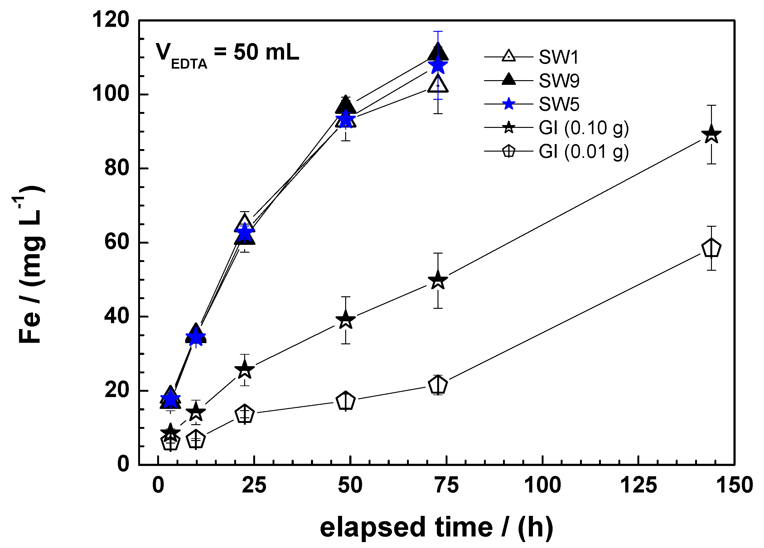
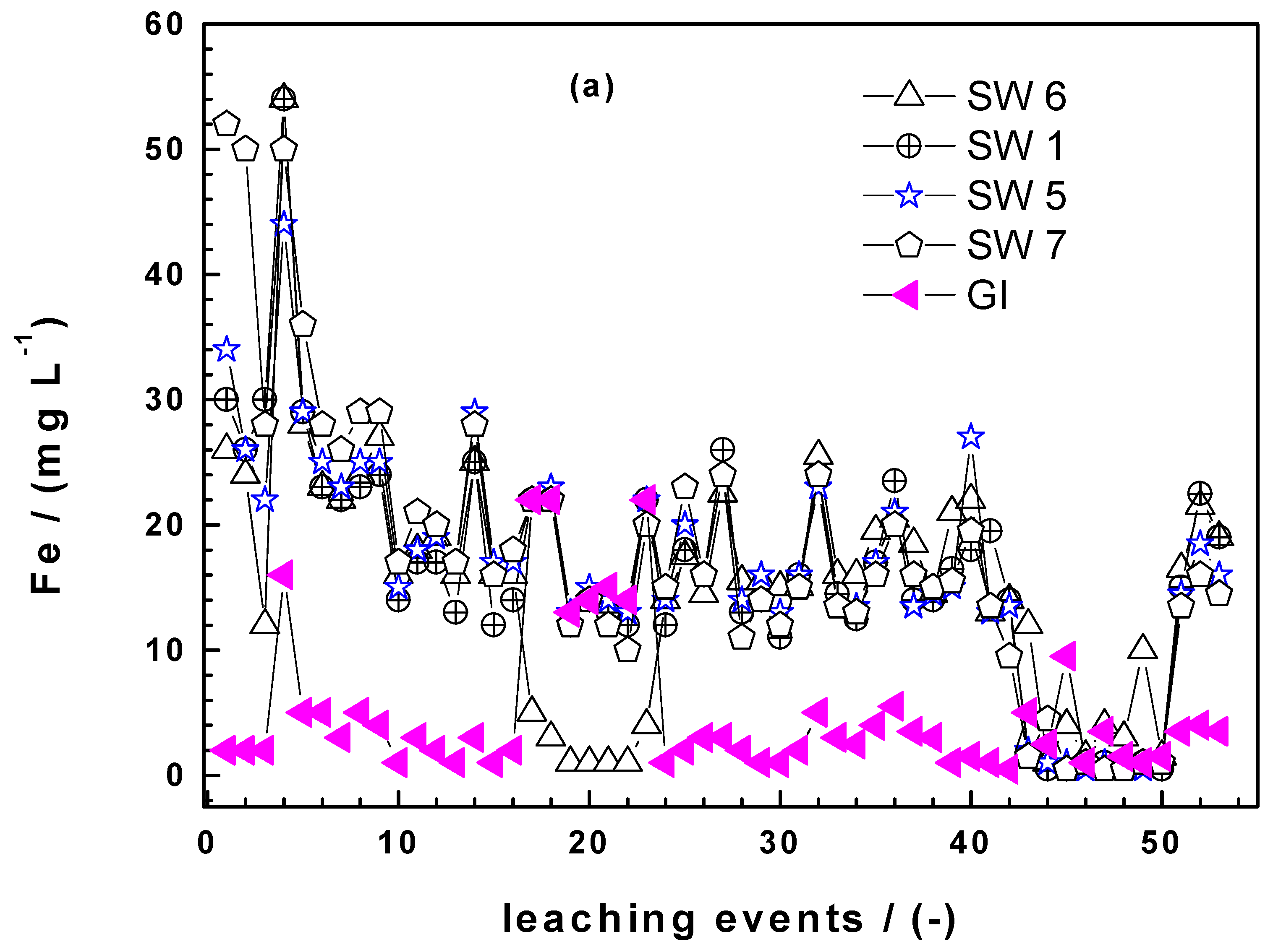
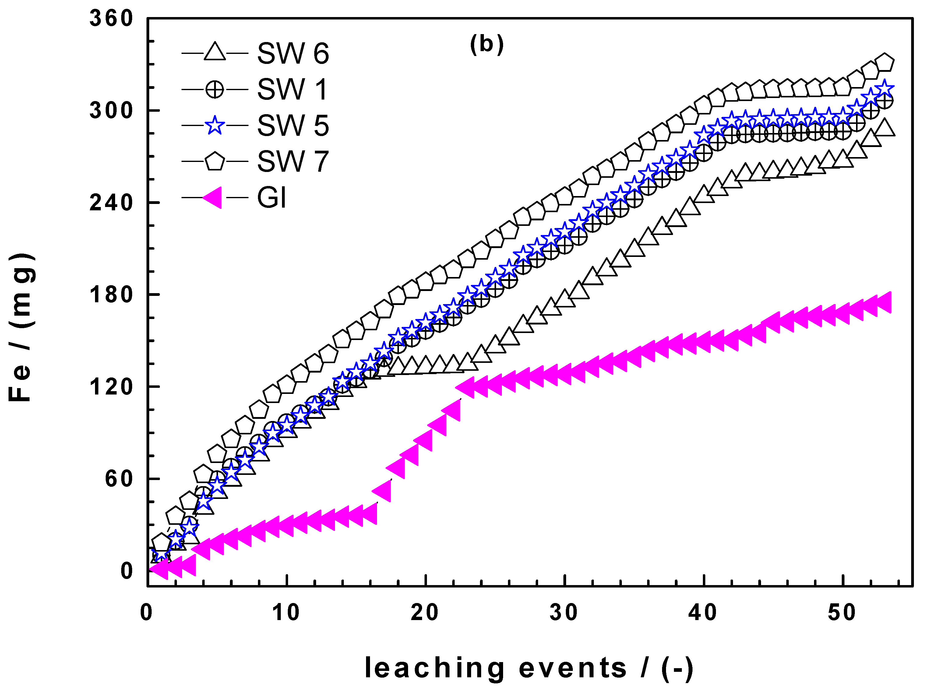
3.1.3. Column Leaching Studies
3.2. MB Discoloration
3.3. Water Defluoridation
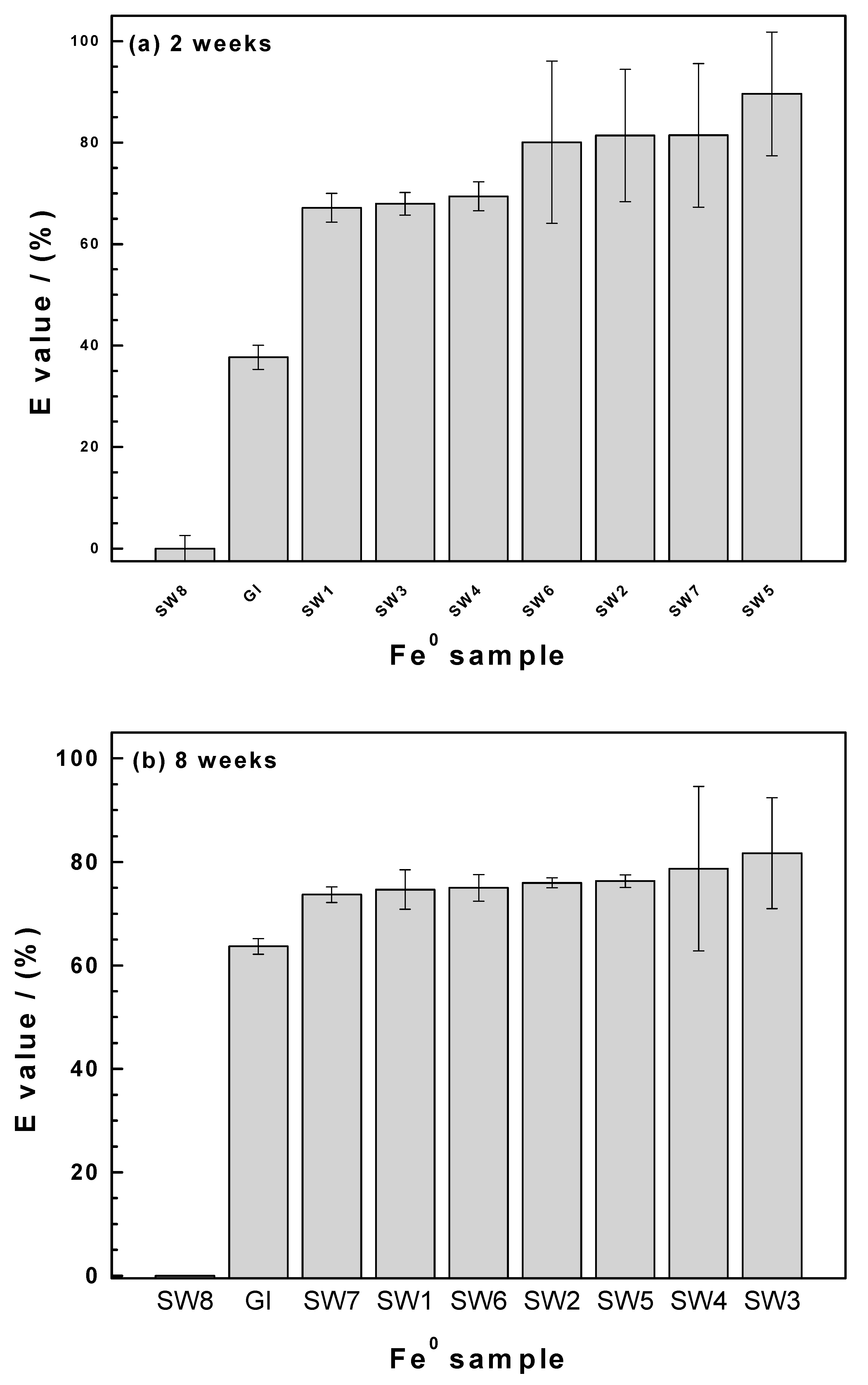
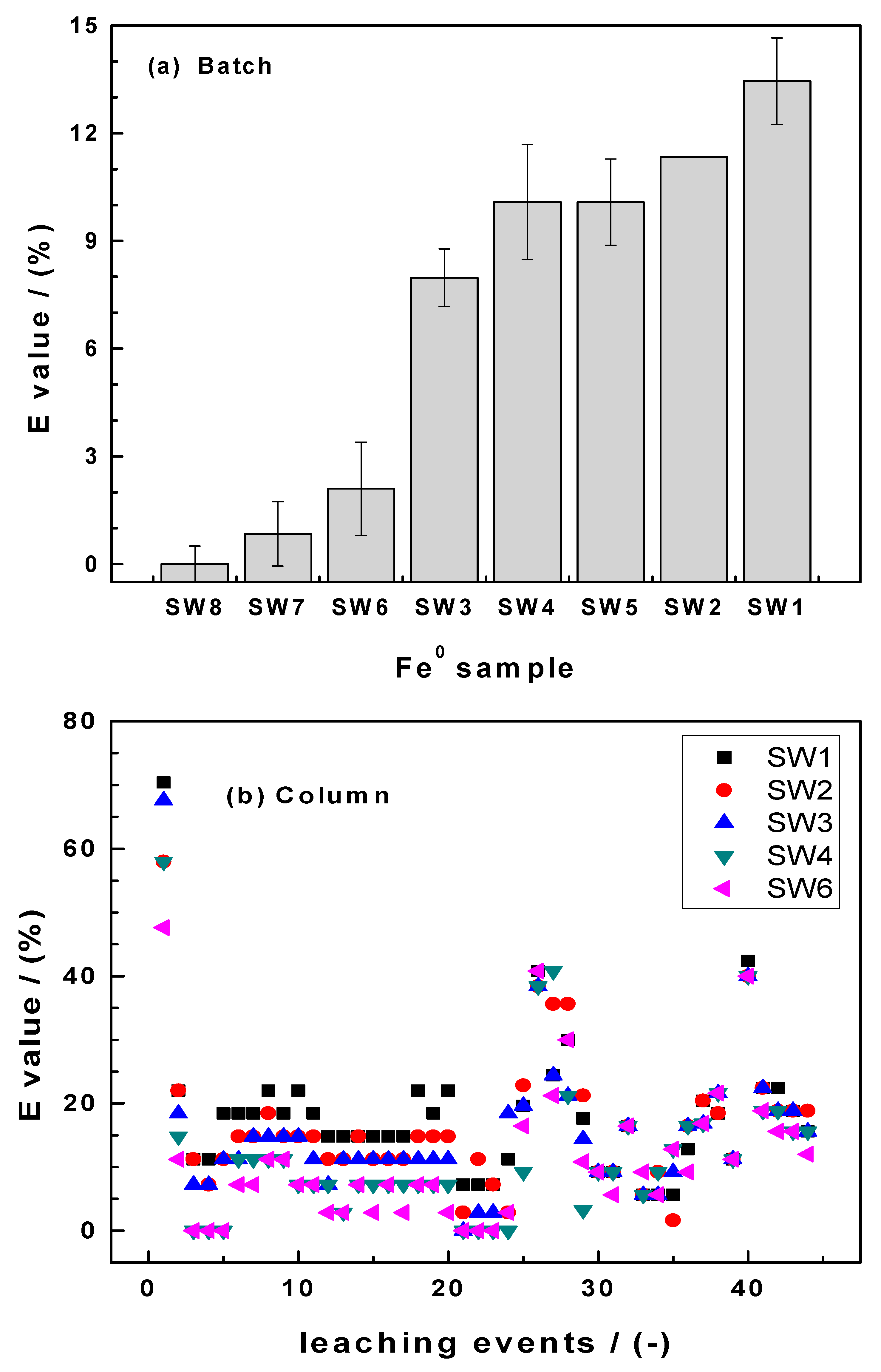
3.3.1. Batch Experiments
3.3.2. Column Experiments
3.4. Discussion
3.4.1. Research in Progress
3.4.2. Significance of the Results
4. Conclusions
Author Contributions
Funding
Acknowledgments
Conflicts of Interest
References
- Bischof, G. The Purification of Water: Embracing the Action of Spongy Iron on Impure Water; Bell and Bain: Glasgow, UK, 1873; 19p. [Google Scholar]
- Bischof, G. On putrescent organic matter in potable water. Proc. R. Soc. Lond. 1877, 26, 258–261. [Google Scholar]
- Bischof, G. On putrescent organic matter in potable water II. Proc. R. Soc. Lond. 1878, 27, 152–156. [Google Scholar]
- Notter, J.L. The purification of water by filtration. Br. Med. J. 1878, 12, 556–557. [Google Scholar] [CrossRef]
- Nichols, W.R. Water Supply, Considered Mainly from a Chemical and Sanitary Standpoint; John Wiley & Sons: New York, NY, USA, 1883; 260p. [Google Scholar]
- Anderson, W. On the purification of water by agitation with iron and by sand filtration. J. Soc. Arts 1886, 35, 29–38. [Google Scholar] [CrossRef]
- Devonshire, E. The purification of water by means of metallic iron. J. Frankl. Inst. 1890, 129, 449–461. [Google Scholar] [CrossRef]
- Antia, D.D.J. Sustainable zero-valent metal (ZVM) water treatment associated with diffusion, infiltration, abstraction and recirculation. Sustainability 2010, 2, 2988–3073. [Google Scholar] [CrossRef]
- Baker, M. Sketch of the history of water treatment. Am. Water Works Assoc. 1934, 26, 902–938. [Google Scholar] [CrossRef]
- Van Craenenbroeck, W. Easton & Anderson and the water supply of Antwerp (Belgium). Ind. Archaeol. Rev. 1998, 20, 105–116. [Google Scholar]
- Mwakabona, H.T.; Ndé-Tchoupé, A.I.; Njau, K.N.; Noubactep, C.; Wydra, K.D. Metallic iron for safe drinking water provision: Considering a lost knowledge. Water Res. 2017, 117, 127–142. [Google Scholar] [CrossRef]
- Lufingo, M.; Ndé-Tchoupé, A.I.; Hu, R.; Njau, K.N.; Noubactep, C. A novel and facile method to characterize the suitability of metallic iron for water treatment. Water 2019, 11, 2465. [Google Scholar] [CrossRef]
- Ndé-Tchoupé, A.I. Design and Construction of Fe0-Based Filters for Hhouseholds. Ph.D. Thesis, University of Douala, Douala, Cameroon, 2019. (In French). [Google Scholar]
- Lufingo, M. Investigation of Metallic Iron for Water Defluoridation. Master’s Thesis, Nelson Mandela African Institution of Science and Technology, Arusha, Tanzania, 2020. [Google Scholar]
- Dannenberg, R.O.; Potter, G.M. Silver Recovery from Waste Photographic Solutions by Metallic Displacement; Report of Investigations 7117; BuMines: Washington, DC, USA, 1968; 22p. [Google Scholar]
- Anderson, M.A. Fundamental Aspects of Selenium Removal by Harza Process; Rep San Joaquin Valley Drainage Program; US Dep Interior: Sacramento, CA, USA, 1989. [Google Scholar]
- Martins, G.F. Percent oxygen in air. J. Chem. Educ. 1987, 64, 809. [Google Scholar] [CrossRef]
- Gordon, J.; Chancey, K. Steel wool and oxygen: A look at kinetics. J. Chem. Educ. 2005, 82, 1065. [Google Scholar] [CrossRef]
- Vogelezang, M. Steel wool and oxygen: How constant should a rate constant be? J. Chem. Educ. 2006, 83, 214. [Google Scholar] [CrossRef][Green Version]
- Vera, F.; Rivera, R.; Núñez, C. A simple experiment to measure the content of oxygen in the air using heated steel wool. J. Chem. Educ. 2011, 88, 1341–1342. [Google Scholar] [CrossRef]
- Lauderdale, R.A.; Emmons, A.H. A method for decontaminating small volumes of radioactive water. J. Am. Water Works Assoc. 1951, 43, 327–331. [Google Scholar] [CrossRef]
- Lacy, W.J. Removal of radioactive material from water byslurrying with powdered metal. J. Am. Water Works Assoc. 1952, 44, 824–828. [Google Scholar] [CrossRef]
- Sifrin, S.M.; Spivakova, O.M.; Krasnoborod’ko, I.G. On color removal from textile wastewater. Sel. Pap. Leningr. Civ. Eng. Inst. 1971, 69, 112–119. [Google Scholar]
- Sugimoto, S.; Sakaki, T. Study on decontamination of radioactive ruthenium by steel wool in waste solution. Radioisotopes 1979, 28, 361–366. [Google Scholar] [CrossRef][Green Version]
- Tseng, C.L.; Yang, M.H.; Lin, C.C. Rapid determination of cobalt-60 in sea water with steel wool adsorption. J. Radioanal. Nucl. Chem. Lett. 1984, 85, 253–260. [Google Scholar] [CrossRef]
- Albinsson, Y.; Christiansen-Saetmark, B.; Engkvist, I.; Johansson, W. Transport of actinides and Technetium through a bentonite backfill containing small quantities of iron or copper. Radiochim. Acta 1991, 52–53, 283. [Google Scholar]
- Khudenko, B.M. Feasibility evaluation of a novel method for destruction of organics. Water Sci. Technol. 1991, 23, 1873–1881. [Google Scholar] [CrossRef]
- Gould, J.P. The kinetics of hexavalent chromium reduction by metallic iron. Water Res. 1982, 16, 871–877. [Google Scholar] [CrossRef]
- Erickson, A.J. Enhanced Sand Filtration for Storm Water Phosphorus Removal. Master’s Thesis, University of Minnesota, Minneapolis, MN, USA, 2005. [Google Scholar]
- Erickson, A.J.; Gulliver, J.S.; Weiss, P.T. Enhanced sand filtration for storm water phosphorus removal. J. Environ. Eng. 2007, 133, 485–497. [Google Scholar] [CrossRef]
- Erickson, A.J.; Gulliver, J.S.; Weiss, P.T. Phosphate removal from agricultural tile drainage with iron enhanced sand. Water 2017, 9, 672. [Google Scholar] [CrossRef]
- Del Cul, G.D.; Bostick, W.D.; Trotter, D.R.; Osborne, P.E. Technetium-99 removal from process solutions and contaminated groundwater. Sep. Sci. Technol. 1993, 28, 551–564. [Google Scholar] [CrossRef]
- Del Cul, G.D.; Bostick, W.D. Simple method for technetium removal from aqueous solutions. Nucl. Tecknol. 1995, 101, 161. [Google Scholar] [CrossRef]
- James, B.R.; Rabenhorst, M.C.; Frigon, G.A. Phosphorus sorption by peat and sand amended with iron oxides or steel wool. Water Environ. Res. 1992, 64, 699–705. [Google Scholar] [CrossRef]
- Ndé-Tchoupé, A.I.; Crane, R.A.; Mwakabona, H.T.; Noubactep, C.; Njau, K.N. Technologies for decentralized fluoride removal: Testing metallic iron based filters. Water 2015, 7, 6750–6774. [Google Scholar] [CrossRef]
- Campos, V. The effect of carbon steel-wool in removal of arsenic from drinking water. Environ. Geol. 2002, 42, 81–82. [Google Scholar] [CrossRef]
- Cornejo, L.; Lienqueo, H.; Arenas, M.; Acarapi, J.; Contreras, D.; Yáñez, J.; Mansilla, H.D. In field arsenic removal from natural water by zero-valent iron assisted by solar radiation. Environ. Pollut. 2008, 156, 827–831. [Google Scholar] [CrossRef]
- Özer, A.; Altundogan, H.S.; Erdem, M.; Tümen, F. A study on the Cr(VI) removal from aqueous solutions by steel wool. Environ. Pollut. 1997, 97, 107–112. [Google Scholar] [CrossRef]
- Gromboni, C.F.; Donati, G.L.; Matos, W.O.; Neves, E.F.A.; Nogueira, A.R.A.; Nobrega, J.A. Evaluation of metabisulfite and a commercial steel wool for removing chromium (VI) from wastewater. Environ. Chem. Lett. 2010, 8, 73–77. [Google Scholar] [CrossRef]
- Till, B.A.; Weathers, L.J.; Alvarez, P.J.J. Fe(0)-supported autotrophic denitrification. Environ. Sci. Technol. 1998, 32, 634–639. [Google Scholar] [CrossRef]
- Lavania, A.; Bose, P. Effect of metallic iron concentration on end-product distribution during metallic iron-assisted autotrophic denitrification. J. Environ. Eng. 2006, 132, 994–1000. [Google Scholar] [CrossRef]
- Bradley, I.; Straub, A.; Maraccini, P.; Markazi, S.; Nguyen, T.H. Iron oxide amended biosand filters for virus removal. Water Res. 2011, 45, 4501–4510. [Google Scholar] [CrossRef] [PubMed]
- Tepong-Tsindé, R.; Ndé-Tchoupé, A.I.; Noubactep, C.; Nassi, A.; Ruppert, H. Characterizing a newly designed steel-wool-based household filter for safe drinking water provision: Hydraulic conductivity and efficiency for pathogen removal. Processes 2019, 7, 966. [Google Scholar] [CrossRef]
- Li, Z.; Huang, D.; McDonald, L.M. Heterogeneous selenite reduction by zero valent iron steel wool. Water Sci. Technol. 2017, 75, 908–915. [Google Scholar] [CrossRef]
- Hildebrant, B. Characterizing the reactivity of commercial steel wool for water treatment. Freib. Online Geosci. 2018, 53, 1–60. [Google Scholar]
- Mitchell, G.; Poole, P.; Segrove, H.D. Adsorption of methylene blue by high-silica sands. Nature 1955, 176, 1025–1026. [Google Scholar] [CrossRef]
- Btatkeu-K, B.D.; Miyajima, K.; Noubactep, C.; Caré, S. Testing the suitability of metallic iron for environmental remediation: Discoloration of methylene blue in column studies. Chem. Eng. J. 2013, 215–216, 959–968. [Google Scholar]
- Miyajima, K.; Noubactep, C. Impact of Fe0 amendment on methylene blue discoloration by sand columns. Chem. Eng. J. 2013, 217, 310–319. [Google Scholar] [CrossRef]
- Miyajima, K. Optimizing the design of metallic iron filters for water treatment. Freib. Online Geosci. 2012, 32, 1–60. [Google Scholar]
- Reardon, J.E. Anaerobic corrosion of granular iron: Measurement and interpretation of hydrogen evolution rates. Environ. Sci. Technol. 1995, 29, 2936–2945. [Google Scholar] [CrossRef] [PubMed]
- Reardon, E.J. Zerovalent irons: Styles of corrosion and inorganic control on hydrogen pressure buildup. Environ. Sci. Tchnol. 2005, 39, 7311–7317. [Google Scholar] [CrossRef] [PubMed]
- Miehr, R.; Tratnyek, G.P.; Bandstra, Z.J.; Scherer, M.M.; Alowitz, J.M.; Bylaska, J.E. Diversity of contaminant reduction reactions by zerovalent iron: Role of the reductate. Environ. Sci. Technol. 2004, 38, 139–147. [Google Scholar] [CrossRef] [PubMed]
- Kim, H.; Yang, H.; Kim, J. Standardization of the reducing power of zero-valent iron using iodine. J. Environ. Sci. Health A 2014, 49, 514–523. [Google Scholar] [CrossRef]
- Li, S.; Ding, Y.; Wang, W.; Lei, H. A facile method for determining the Fe(0) content and reactivity of zero valent iron. Anal. Methods 2016, 8, 1239–1248. [Google Scholar] [CrossRef]
- Li, J.; Dou, X.; Qin, H.; Sun, Y.; Yin, D.; Guan, X. Characterization methods of zerovalent iron for water treatment and remediation. Water Res. 2019, 148, 70–85. [Google Scholar] [CrossRef]
- Miyajima, K.; Noubactep, C. Effects of mixing granular iron with sand on the efficiency of methylene blue discoloration. Chem. Eng. J. 2012, 200–202, 433–438. [Google Scholar]
- Miyajima, K.; Noubactep, C. Characterizing the impact of sand addition on the efficiency of granular iron for water treatment. Chem. Eng. J. 2015, 262, 891–896. [Google Scholar] [CrossRef]
- Naseri, E.; Ndé-Tchoupé, A.I.; Mwakabona, H.T.; Nanseu-Njiki, C.P.; Noubactep, C.; Njau, K.N.; Wydra, K.D. Making Fe0-Based filters a universal solution for safe drinking water provision. Sustainability 2017, 9, 1224. [Google Scholar] [CrossRef]
- Phukan, M. Characterizing the Fe0/sand system by the extent of dye discoloration. Freib. Online Geosci. 2015, 40, 1–70. [Google Scholar]
- Varlikli, C.; Bekiari, V.; Kus, M.; Boduroglu, N.; Oner, I.; Lianos, P.; Lyberatos, G.; Icli, S. Adsorption of dyes on Sahara desert sand. J. Hazard. Mater. 2009, 170, 27–34. [Google Scholar] [CrossRef]
- Saywell, L.G.; Cunningham, B.B. Determination of iron: Colorimetric o-phenanthroline method. Ind. Eng. Chem. Anal. Ed. 1937, 9, 67–69. [Google Scholar] [CrossRef]
- Buck, R.P.; Rondinini, S.; Covington, A.K.; Baucke, F.G.K.; Brett, C.M.A.; Camoes, M.F.; Milton, M.J.T.; Mussini, T.; Naumann, R.; Pratt, K.W.; et al. Measurement of pH. Definition, standards, and procedures (IUPAC Recommendations 2002). Pure Appl. Chem. 2002, 74, 2169–2200. [Google Scholar] [CrossRef]
- Noubactep, C.; Meinrath, G.; Dietrich, P.; Sauter, M.; Merkel, B. Testing the suitability of zerovalent iron materials for reactive Walls. Environ. Chem. 2005, 2, 71–76. [Google Scholar] [CrossRef]
- Ibanez, J.G.; Gonzalez, I.; Cardenas, M.A. The effect of complex formation upon the redox potentials of metallic ions: Cyclic voltammetry experiments. J. Chem. Educ. 1998, 65, 173–175. [Google Scholar] [CrossRef]
- Rizvi, M.A. Complexation modulated redox behavior of transition metal systems. Rus. J. Gen. Chem. 2015, 85, 959–973. [Google Scholar] [CrossRef]
- Heimann, S. Testing granular iron for fluoride removal. Freib. Online Geosci. 2018, 52, 1–80. [Google Scholar]
- Heimann, S.; Ndé-Tchoupé, A.I.; Hu, R.; Licha, T.; Noubactep, C. Investigating the suitability of Fe0 packed-beds for water defluoridation. Chemosphere 2018, 209, 578–587. [Google Scholar] [CrossRef]
- Ndé-Tchoupé, A.I.; Nanseu-Njiki, C.P.; Hu, R.; Nassi, A.; Noubactep, C.; Licha, T. Characterizing the reactivity of metallic iron for water defluoridation in batch studies. Chemosphere 2019, 219, 855–863. [Google Scholar] [CrossRef]
- Van Genuchten, C.M.; Behrends, T.; Stipp, S.L.S.; Dideriksen, K. Achieving arsenic concentrations of <1 µg/L by Fe(0) electrolysis: The exceptional performance of magnetite. Water Res. 2020, 168, 115170. [Google Scholar]
- Lavine, B.K.; Auslander, G.; Ritter, J. Polarographic studies of zero valent iron as a reductant for remediation of nitroaromatics in the environment. Microchem. J. 2001, 70, 69–83. [Google Scholar] [CrossRef]
- Nesic, S. Key issues related to modelling of internal corrosion of oil and gas pipelines—A review. Corros. Sci. 2007, 49, 4308–4338. [Google Scholar] [CrossRef]
- Lazzari, L. General aspects of corrosion. In Encyclopedia of Hydrocarbons; Chapter 9.1; Istituto Enciclopedia Italiana: Rome, Italy, 2008; Volume V. [Google Scholar]
- Moraci, N.; Lelo, D.; Bilardi, S.; Calabrò, P.S. Modelling long-term hydraulic conductivity behaviour of zero valent iron column tests for permeable reactive barrier design. Can. Geotech. J. 2016, 53, 946–961. [Google Scholar] [CrossRef]
- Santisukkasaem, U.; Das, D.B. A non-dimensional analysis of permeability loss in zero-valent iron permeable reactive barrier (PRB). Transp. Porous Media 2019, 126, 139–159. [Google Scholar] [CrossRef]
- Magomnang, A.A.S.; Villanueva, E.P. Removal of hydrogen sulfide from biogas using dry desulfurization systems. In Proceedings of the International Conference on Agricultural, Environmental and Biological Sciences (AEBS-2014), Phuket, Thailand, 24–25 April 2014; pp. 77–80. [Google Scholar]
- Magomnang, A.; Villanueva, E.P. Utilization of the uncoated steel wool for the removal of hydrogen sulfide from biogas. Int. J. Min. Metall. Mech. Eng. 2015, 3, 108–111. [Google Scholar]
- Riyadi, U.; Kristanto, G.A.; Priadi, C.R. Utilization of steel wool as removal media of hydrogen sulfide in biogas. IOP Conf. Ser. Earth Environ. Sci. 2018, 105, 012026. [Google Scholar] [CrossRef]
- Noubactep, C. The fundamental mechanism of aqueous contaminant removal by metallic iron. Water SA 2010, 36, 663–670. [Google Scholar] [CrossRef]
- Gheju, M. Hexavalent chromium reduction with zero-valent iron (ZVI) in aquatic systems. Water Air Soil Pollut. 2011, 222, 103–148. [Google Scholar] [CrossRef]
- Ghauch, A. Iron-based metallic systems: An excellent choice for sustainable water treatment. Freib. Online Geosci. 2015, 32, 1–80. [Google Scholar]
- Westerhoff, P.; James, J. Nitrate removal in zero-valent iron packed columns. Water Res. 2003, 37, 1818–1830. [Google Scholar] [CrossRef]
- Noubactep, C.; Schöner, A.; Woafo, P. Metallic iron filters for universal access to safe drinking water. Clean Soil Air Water 2009, 37, 930–937. [Google Scholar] [CrossRef]
- Nanseu-Njiki, C.P.; Gwenzi, W.; Pengou, M.; Rahman, M.A.; Noubactep, C. Fe0/H2O filtration systems for decentralized safe drinking water: Where to from here? Water 2019, 11, 429. [Google Scholar] [CrossRef]
- Hu, R.; Yang, H.; Tao, R.; Cui, X.; Xiao, M.; Konadu-Amoah, B.; Cao, V.; Lufingo, M.; Soppa-Sangue, N.P.; Ndé-Tchoupé, A.I.; et al. Metallic Iron for Environmental Remediation: Starting an Overdue Progress in knowledge. Water 2020, in press. [Google Scholar]


| Material Code | Size | Grade | Thickness (µm) | Trade Name |
|---|---|---|---|---|
| SW1 | fine | 00 | 40 | RASKO (Germany) |
| SW2 | medium | 0 | 50 | RASKO (Germany) |
| SW3 | medium | 1 | 60 | RASKO (Germany) |
| SW4 | medium | 2 | 75 | RASKO (Germany) |
| SW5 | fine | 00 | 40 | Champion (Kenya) |
| SW6 | fine | 00 | 40 | SOKONI (Kenya) |
| SW7 | fine | 00 | 40 | BOBBY MAT (Germany) |
| SW8 | coarse | 2 | 75 | Stainless steel Topfreiniger (Germany) |
| SW9 | fine | 00 | 40 | SOCAPINE (Cameroon) |
| SW10 | extra fine | 000 | 35 | Grand Menage (Cameroon) |
| SW11 | fine | 0 | 50 | Stainless steel SUPRAWISCH (China) |
| SW12 | medium | 1 | 60 | LIJIA (China) |
| SW13 | fine | 0 | 50 | Grand Menage (Cameroon) |
| SW14 | coarse | 2 | 75 | MAGIC MAMY (Cameroon) |
| SW15 | coarse | 3 | 90 | Generic steel wool (Cameroon) |
| Column 1 | Column 2 | Column 3 | Column 4 | Column 5 | |
|---|---|---|---|---|---|
| Steel Wool | SW 1 | SW 2 | SW 3 | SW 4 | SW 6 |
| Mass (g) | 1.985 | 1.989 | 2.006 | 2.009 | 1.996 |
| Fe0 | kEDTA | b | R2 |
|---|---|---|---|
| (µg h−1) | (µg) | (−) | |
| SW 1 | 78.4 | 552.9 | 0.8851 |
| SW 2 | 111.7 | 160.0 | 0.9984 |
| SW 3 | 113.0 | 435.8 | 0.9761 |
| SW 4 | 110.9 | 322.4 | 0.9873 |
| SW 5 | 106.9 | 393.0 | 0.9707 |
| SW 6 | 130.8 | 282.6 | 0.9881 |
| SW 7 | 112.6 | 261.6 | 0.9960 |
| SW 8 | 0.0 | 0.0 | n.a. |
| SW9 | 84.9 | 289.4 | 0.9944 |
| SW10 | 108.3 | 516.7 | 0.9970 |
| SW11 | 0.0 | 0.0 | n.a. |
| SW12 | 28.7 | 77.9 | 0.9838 |
| SW13 | 31.2 | −170.8 | 0.8010 |
| SW14 | 24.4 | −138.4 | 0.9583 |
| SW15 | 20.1 | 132.6 | 0.7427 |
| GI | 3.7 | −10.3 | 0.9396 |
© 2020 by the authors. Licensee MDPI, Basel, Switzerland. This article is an open access article distributed under the terms and conditions of the Creative Commons Attribution (CC BY) license (http://creativecommons.org/licenses/by/4.0/).
Share and Cite
Hildebrant, B.; Ndé-Tchoupé, A.I.; Lufingo, M.; Licha, T.; Noubactep, C. Steel Wool for Water Treatment: Intrinsic Reactivity and Defluoridation Efficiency. Processes 2020, 8, 265. https://doi.org/10.3390/pr8030265
Hildebrant B, Ndé-Tchoupé AI, Lufingo M, Licha T, Noubactep C. Steel Wool for Water Treatment: Intrinsic Reactivity and Defluoridation Efficiency. Processes. 2020; 8(3):265. https://doi.org/10.3390/pr8030265
Chicago/Turabian StyleHildebrant, Benjamin, Arnaud Igor Ndé-Tchoupé, Mesia Lufingo, Tobias Licha, and Chicgoua Noubactep. 2020. "Steel Wool for Water Treatment: Intrinsic Reactivity and Defluoridation Efficiency" Processes 8, no. 3: 265. https://doi.org/10.3390/pr8030265
APA StyleHildebrant, B., Ndé-Tchoupé, A. I., Lufingo, M., Licha, T., & Noubactep, C. (2020). Steel Wool for Water Treatment: Intrinsic Reactivity and Defluoridation Efficiency. Processes, 8(3), 265. https://doi.org/10.3390/pr8030265