Abstract
Waste heat recovery plays an important role in energy source management. Organic Rankine Cycle (ORC) can be used to recover low-temperature waste heat. In the present work a sample power plant waste heat was used to operate an ORC. First, two pure working fluids were selected based on their merits. Four possible thermodynamic models were considered in the analysis. They were defined based on where the condenser and evaporator temperatures are located. Four main thermal parameters, evaporator temperature, condenser temperature, degree of superheat and pinch point temperature difference were taken as key parameters. Levelized energy cost values and exergy efficiency were calculated as the optimization criteria. To optimize exergy and economic aspects of the system, Strength Pareto evolutionary algorithm II (SPEA II) was implemented. The Pareto frontier solutions were ordered and chose by TOPSIS. Model 3 outperformed all other models. After evaluating exergy efficiency by mixture mass fraction, R245fa [0.6]/Pentane [0.4] selected as the most efficient working fluid. Finally, every component’s role in determining the levelized energy cost and the exergy efficiency and were discussed. The turbine, condenser and evaporator were found as the costliest components.
1. Introduction
Designing an optimal energy recovery system has become a hot spot for energy management researches. The rapid expansion of growing industries and their high demand for green energy have made energy recovery of paramount importance to today’s companies. Recovering the wasted heat, which usually has a low temperature, by optimally converting it into other forms of energy like electrical energy is a subject of ongoing debates. The Organic Rankine Cycle (ORC) has been known as one of the most effective methods for the recovering process. When using an ORC for recovering wasted energy, an evaporator supplants the boiler and heats the working fluid. In the ORC an organic fluid used as the working fluid, which made the cycle capable of operating with low-temperature sources like biomass, geothermal, and solar energy. The cycle can be operated with industries’ wasted energy and converts it into mechanical work.
Demands for energy optimization have been urged since the early 1970s. It consists of three essential aspects, including energy, economic, and environmental efficiency. Industrial countries have made a vast fortune using energy optimization while preserving and improving environmental standards in the last decades. Nowadays, energy management and optimization perceive as a new source of energy. To optimize a system, its parameters and components should be optimally selected.
Many efforts have been made to optimize the ORC for different situations. Li et al., 2012 [1] conducted an exergo-economic analysis along with condenser performance optimization for a binary mixture of vapors in the ORC system. They showed that with increasing the difference of the temperature ratios, the optimal number of transfer units decreases, leading to the heat capacity ratio rise [1]. El-Emam and Dincer, 2013 [2] optimized a geothermal ORC based on the heat exchanger’s total surface area parameter and performed an exergo-economic analysis of the system with the heat source temperature of 165◦ Celsius. They used Isobutane as the working fluid and reached the energy and exergy efficiency of 16.37% and 48.8, respectively [2]. Khaljani et al., 2015 [3] carried out an exergo-economic analysis of a combined gas turbine and an ORC. They found that an increase in the condenser temperature and Pinch point temperature difference can significantly decrease the first and second law efficiencies while increasing the total cost [3]. Yari et al., 2015 [4] performed an Exergo-economic comparison of trilateral power cycle (TPW), the Kalina cycle, and the ORC. They found Butane to be the most economically efficient gas when using the working fluid of both ORC and TPW. Yang et al., 2015 [5] thermo-economically optimized a diesel engine waste heat recovery ORC system. They have found R245fa- also known as Pentafluoropropane- the most efficient working fluid used in a waste heat recovery ORC system [5]. The same result was found in other researches [6,7]. Scardigno et al., 2016 [8] examined the thermo-economic performances for an ORC fed by solar energy. They introduced heat exchangers as the most inefficient components of the system [8]. Wang et al. 2016 [9] conducted a geothermal ORC Multi-objective optimization along with grey relational analysis. They found the Pareto frontier as an effective way of comprehensively comparing ORCs [9]. Nazari et al., 2016 [10] carried out an exergo-economic multi-objective optimization of a combined steam-organic Rankine cycle. They revealed that the combined cycle with R152a has the best performance among R124, R152a, and R134a fluids [10]. Zou et al., 2016 [11] analyzed the performance of the partial evaporating ORC with zeotropic mixtures. They proposed a partial evaporating ORC with R245fa/R227ea, which can outperform the traditional subcritical ORC with R227ea by generating 24.7% more power [11]. Wang et al., 2017 [12] enhanced the performance of ORC with two-stage evaporation based on energy and exergy analysis. They have found that even though the two-stage evaporation improved the evaporation procedure, it deteriorated the condensation, pressurization, and expansion processes [12]. Bufi et al., 2017 [13] optimized ORC using both the single-objective genetic algorithm and the multi-objective Non-dominated sorting genetic algorithm II (NSGA-II). They found Toluene as a compelling choice for heat exchanger efficiency [13]. Scardigno et al., 2015 [14] used the multi-objective NSGAII optimization algorithm to find the hybrid organic Rankine plant for solar and lowgrade energy sources with the highest first and second law efficiencies and the lowest levelized energy cost. They found Cyclopropane as the most efficient working fluids, with a power output greater than 100 kW [14].
In this research, we performed a thermo-economic optimization of ORC for the heat recovery of a sample power plant. As a mixture, working fluid is used, four possible thermodynamic models were considered. They were defined based on where the condenser and evaporator temperatures are located. Exergy efficiency and levelized energy cost values were calculated for every component of the system to investigate their relative role in system performance. To optimize the exergy and economic aspects of the system, a multi-objective Strength Pareto Evolutionary Algorithm II (SPEA II) [15] was used, and Pareto frontier answers were ordered and chose by Technique for Order of Preference by Similarity to Ideal Solution (TOPSIS) [16]. Four main thermal parameters, evaporator temperature, condenser temperature, degree of superheating and pinch point temperature difference, were taken as critical parameters. This paper is organized in the following order; first, detail explanations of the system are discussed. Then, the optimization algorithm is introduced, and after that, the results are analyzed.
2. Designing and Formulation
In this section, we present the thermodynamic and economical formulation of the system. Four realistic thermodynamic models have been investigated to represent the sample power plant’s wasted energy. The Pinch point temperature difference of a heat exchanger can be located at either end of it. The position of the Pinch point temperature difference for both evaporator and condenser can change the temperature-entropy diagram and the system outcomes. While the saturated liquid temperature and saturated vapor temperature at evaporator pressure are equal for pure working fluids, it is not the case for mixture working fluids due to the Glide temperature difference. The evaporator temperature for mixture working fluids can be set to either saturated liquid temperature or saturated vapor temperature at evaporator pressure. Similarly, the condenser temperature for mixture working fluids can be set to either saturated liquid temperature or saturated vapor temperature at condenser pressure. For mixture working fluids, unlike pure working fluids, the locations of condensing dew point temperature and evaporating bubble point temperature have a decisive effect on the cycle. The system constraints determine the Pinch point temperature difference location [17]. Regarding their possible locations, four models for mixture working fluids are considered [17]. The temperature-entropy diagrams of the four different models are illustrated in Figure 1. In the first model, the evaporator temperature set to the saturated vapor temperature at evaporator pressure and the condenser temperature set to the saturated liquid temperature at condenser pressure. In the second model, both the evaporator and condenser temperatures set to the saturated vapor temperature. In the third model, both the evaporator and condenser temperatures set to the saturated liquid temperature. Finally, for the fourth model, the evaporator temperature set to the saturated liquid and the condenser temperature set to the saturated vapor temperature.

Figure 1.
The temperature-entropy diagram of the four considered models. The green diagrams represent the pure fluid cycle, while the orange diagrams represent the mixture working fluid [17].
2.1. System Thermodynamic
The first and second laws of thermodynamics and their dependent concepts are the crucial factors in designing a thermodynamic system. The first law of thermodynamic relation for a control volume is as below
The subscribe CV is for emphasizing on control volume heat transfer. The entropy relation for a control volume is written as:
The exergy efficiency of the system can be calculated as follows [18,19].
2.2. Exergo-Economic Formulation
In a typical exergy-economic analysis, a levelized cost for a system specified using the following relations [18].
where is the product cost rate, in the fuel cost rate, is the initial investment rate and is the operation and maintenance cost rate. In a cost-effective formulation, one should link the cost to the exergy of every flow [18]. For every flow we have
The cost of exchange heat and mechanical work we have
where , , , and represented exergy of executed mechanical work, exiting flow exergy, entering flow exergy and exergy of the transferred heat, respectively. , , , and represent their average costs. One of the main equations here is the cost balance equation that should be written for every component of the system and liked its entering and exiting costs with its operation and maintenance cost. This equation for every component (subscribe k) is written as follows [19].
Where
Tsatsaronis et al., 1994 [20] proposed the following equation for determining the price of the system components in a time scale
Where is capital recovery factor, is the operating and maintenance and is the interest rate. and are calculated using the following equations [21].
Where represented the inflation rate and is the working years of the system and
We can rewrite Equation (10) for every component, but this time we consider the fuel cost and the production and drop in the cost balance equation [18].
The average cost of fuel and production for the th component of the system can be written as [18]:
We can consider the exergy drop using two estimations [18], the first one used:
In this case, the average fuel cost is considered for the exergy drop flow. The second one used:
In this case, the average product exergy cost is considered for the exergy drop flow. Another critical parameter to consider is the exergy destruction cost, which is also known as a hidden cost. When the average product exergy stayed constant and the average fuel cost considered independent of exergy destruction, one can determine the exergy destruction cost using [18]:
And when the fuel exergy stayed constant and the average product exergy considered independent of the exergy destruction, we can calculate the exergy destruction as:
One useful parameter in optimizing the heat systems is the relative cost difference. This parameter can be determined using the following relation [18].
In an iterative process for the exergo-economic optimization, if the fuel cost of a component changes the relative cost difference can be calculated using [18]:
The exergo-economic coefficient can be defined as [18]:
The objective function of this research is defined as:
The component product exergy flow rate and the average cost per unit of fuel are assumed to remain constant for every component.
Zero exergy waste assume for the system components
The levelized energy cost can be calculated using the following equation.
2.3. Working Fluid
Choosing the appropriate working fluid is one of the most important decisions when designing the system. In this research, a fluid screening approach is used for working fluid selection. Choosing criteria like fluid’s effects on system output efficiency, minimizing fluid reliant damage to system components, appropriate viscosity and density, fluid safety, environmental impacts, supply cost, availability, and fluid temperature range for thermodynamic cycle were considered. It is almost impossible to find an organic fluid that satisfies all the desired criteria. One practical way to tackle this challenge is the use of combined fluids instead of pure fluids. It would equip us with a fluid that can have the advantages of its constituents. Moreover, the mixed fluid would provide a more significant Glide temperature difference that happened at phase change at constant pressure, which increases the synchronization between the temperature curve of the heat source and the working fluid. It causes a temperature increase in the evaporator outputs while decreasing the condenser output temperature. Therefore, it helps in reducing exergy destruction.
Numbers of different working fluids were examined based on desired criteria and eventually, the combination of the two organic fluids of Pentane and R24fa (also known as Pentafluoropropane) choose as the working fluid. Pentane has low cost, low evaporation temperature, and high safety. Even though R24fa has a high supply cost, it has a low Global Warming Potential (GWP) with no Ozone Depletion Potential (ODP). Both Pentane and R24fa are dry working fluids. A combination of these two fluids made it possible to exploit their individual merits simultaneously. The temperature-entropy diagram of these two fluid illustrated in Figure 2 and their characteristics are presented in Table 1.
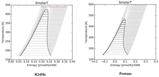
Figure 2.
The temperature-entropy diagram of the two pure organic fluid R245fa (left) and Pentane (right).

Table 1.
The characteristics of the pure working fluids and their combination.
2.4. Implementation
When performing a combined thermodynamic and thermo-economic optimization, it is expected to simultaneously minimize the thermodynamic inefficiencies and system costs. Thus, in an optimal system, there has to be a trade-off between thermodynamic inefficiencies like exergy destruction and the cost efficiency of the system. In order to perform an optimization process, the optimization problem should be formulated in the first step.
For formulating an optimization problem, we should define the optimization variables and criteria. For thermo-economic optimization, the variable should be thermodynamical variables that independently linked to the system’s efficiency and costs. Here, we choose four main thermal parameters, evaporator temperature, condenser temperature, degree of superheating, and pinch point temperature difference as the optimization variable. The exergy efficiency (Equation (3)) of the system and the levelized energy cost (Equation (30)) have been used as the optimization criteria.
Since we focused on optimizing the system’s components here, the external conditions are just introduced to the problem. The waste heat from exhaust provided the heat for the evaporator. Hence, the exhaust gas temperature, its constituents, and the mass flow rate are important factors in the optimization problem. In this study, a constant heat exchanger was used for transferring the source heat to the ORC. In other words, the heat exchanger cost and its effects on the system’s thermo-economic weren’t considered in the optimization procedure. The crucial assumptions that hold for the system are presented in Table 2 [22].
Table 2.
System assumptions.
The purchase cost of system components was extracted from Baasel and von Matt, 1976 [23] and converted to 2019 September [24] (the date of conducting the research). The annual inflation rate was set to 10%, and the useful life of the system components was considered to be ten years. The operation and maintenance cost was set equal to 2% of the investment cost. The system was assumed to work 24-hour and was set equal to 8000 working hours per year [17,25].
3. Optimization
To obtain the most efficient design of the system, we need to deal with an optimization procedure. The multi-objective Strength Pareto Evolutionary Algorithm II (SPEA II) was used to simultaneously optimize the system for both exergy and economic criteria and obtain the Pareto frontier. SPEA II is a very efficient multi-objective algorithm compared to other alternative approaches. It preserved the accuracy while having a low computational cost and outperformed other comparable algorithms [26,27]. The solutions in the Pareto frontier were ordered based on their similarity to the ideal solution, and the closest one chooses as the best solution.
3.1. SPEA II
Strength Pareto evolutionary algorithm (SPEA) is an outgrowth of the original genetic algorithm and a commonly used evolutionary algorithm for multi-objective optimizations [15]. SPEAII is an upgrade of the SPEA, which can lead us to the Pareto solutions [15]. It exploited the use of two population sets in each iteration (); main () and archive () population sets. The archive population set (with the size of ) was expected to converge toward Pareto frontier solutions with iterations (maximum number of iterations). The essential steps of the algorithm used here are detailed in the following paragraph [15] and the algorithm flowchart illustrated in Figure 3.
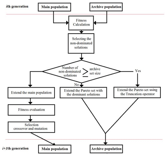
Figure 3.
Strength Pareto evolutionary algorithm II (SPEA II) algorithm flowchart.
- Initiation: The initial main population (with the size of ) generated and the archive population set empty .
- Fitness assignment: The fitness value for every individual solution in the main and archive population set was calculated from the strength Pareto values for each solution. The strength Pareto values can be calculated for the th solution using the following relation:where, represents the cardinality of a set and denoted to the Pareto dominance relation. According to Equation (31), the strength Pareto value has a lower strength for a dominant solution. The fitness value for the th solution can be calculated using the following equation:where, the raw fitness values for the th solution calculated as follow:The density information is added to prevent the algorithm failure when using the raw fitness values with the solutions that do not dominate each other. It represents the density using the th nearest neighbor distance. can be calculated usingwhere is the space distance from the th solution and its th nearest neighbor. We also set .
- Environmental selection: duplicate all the non-dominated solutions in and to . If there are more non-dominated solutions than , then the algorithm reduced them using the truncation operator. In the other case, the algorithm filled . with the dominant solutions in and .
- Termination: if the stopping criteria satisfied (here ), stop the process and present the archive population as the Pareto frontier, otherwise perform the following steps.
- Mating selection: creating the mating pool by binary tournament selection from the solutions in .
- Variation: to create the new main population , apply the Mutation and crossover operators to the mating pool, and go back to the second step.
3.2. SPEA II Parameters Specification
Some parameters need to be defined by the user for operating the SPEA II. The specifications of the algorithm are presented in Table 3, and the optimization variables’ changing range are introduced in Table 4.
Table 3.
Parameters used in SPEA II.
Table 4.
Optimization variables changing range.
3.3. TOPSIS
Technique for Order of Preference by Similarity to Ideal Solution (TOPSIS) was developed by Hwang and Yoon, 1981 [16] and is one of the best multi-criteria decision analysis methods. It performed to find a solution that has the lowest distance in the objective space (has the most similarity) to the ideal solution while placed farthest apart from the worst solution. The ideal solution is a solution where both optimization criteria have the highest values, and the worst solutions have the lowest criteria values in the objective space. The weighted distance in the objective space was used as the similarity measure. Here, we gave the same weight to both the exergy efficiency and levelized energy cost, for both criteria have the same importance in the optimization process. final solutions obtained from the SPEA II were examined and ordered using the TOPSIS method and the solution with the best score chose as the best possible solution.
4. Results and Discussion
In this section, the research outcomes were presented. Before addressing the optimization results, we validate the problem formulation against the experimental result of Kolahi et al., 2016 [28] analysis.
4.1. Validation
In order to validate the methodology of this study and ensure the reliability of the results, we simulated the outcomes of a published analysis with the current methodology. Kolahi et al., 2016 [28] conducted an exergo-economic analysis for ORC with mixture fluid as the working fluid. Their results were simulated with the same conditions using the formulation used in this study. Figure 4 illustrated the simulated and the reference exergy efficiency for both R236ea/Isohexane and R245fa/Hexane working fluids as a function of the fluids mixing ratio. As observed in Figure 4, the result of the simulation and the reference result are in good agreement. The maximum deviation between the simulated and the reference exergy efficiency is 2.2% for R236ea/Isohexane and 1.2% for R245fa/Hexane.
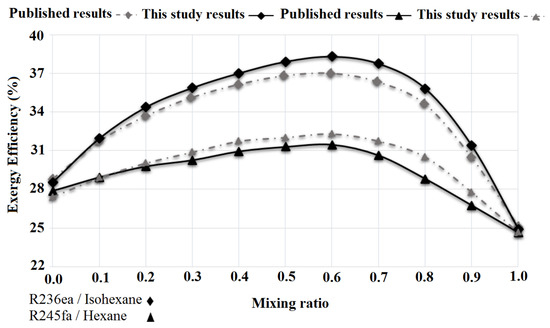
Figure 4.
Comparison of the simulated exergy efficiency to the similar previously published data [28] for both R236ea/Isohexane and R245fa/Hexane working fluids.
Similar to Figure 4, Figure 5 showed the simulated and the previously published data System Investment Cost (SIC) for both R236ea/Isohexane and R245fa/Hexane working fluids as a function of the evaporator temperature. SIC is calculated as the sum of the system’s component investment cost. The mixing ratio for both working fluids is held constant at 0.5. The result of the simulation and the reference result produced similar curves. The maximum deviation between the simulated and reference SCI is 0.7% for R236ea/Isohexane and 1.8% for R245fa/Hexane.
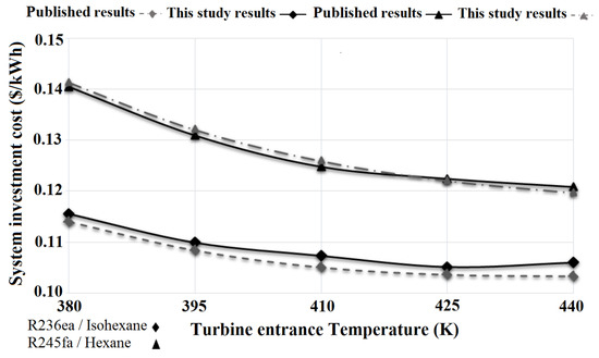
Figure 5.
Comparison of the simulated System Investment Cost (SIC) to the similar previously published data [28] for both R236ea/Isohexane and R245fa/Hexane working fluids.
The comparison of the simulated results with the previously published outcomes showed the excellent reliability of the formulation used in this study.
4.2. Optimization Results and Discussion
Figure 6 showed the Pareto frontier solutions obtained by performing the optimization procedure for four predefined models with a fixed mixing ratio of 0.5 for Pentane/R24fa working fluids in the objective space. The best possible solution obtained by the TOPSIS method is highlighted by the red cycles. As observed in Figure 6, considering the cost efficiency, model 3 and 4 showed the best and worst behavior, respectively While models 2 and 4 revealed moderate behaviors. Considering the exergy efficiency, models 4 and 3 showed the worst and best behaviors, respectively, while models 1 and 2 exhibited fair behaviors. Thus, we chose the model 3 as the preferable model. Figure 7 demonstrated the exergy efficiency of model 3 as a function of working fluid mixing ratio (other optimization variables are held constant). From Figure 7, it can be inferred that increasing the R24fa ratio in the mixture to 0.6, increase the exergy efficiency while further grow in the R24fa mixing ratio, decrease the exergy efficiency of model 3. Hence, the Pentane [0.6]/R24fa [0.4] mixture considered as the mixing ratio with the most exergy efficiency. Figure 8 illustrated the Pareto frontier solutions in the objective space for model 3 with three different working fluids, pure Pentane, pure R24fa, and the combined Pentane [0.6]/R24fa [0.4]. Considering the Pareto frontier solutions in Figure 8, It can be seen that using the Pentane [0.6]/R24fa [0.4] as the working fluid significantly increased the exergy efficiency of the system while imposing the maximum cost on the system. Table 5 presented the detail of the best possible solutions highlighted in Figure 8.
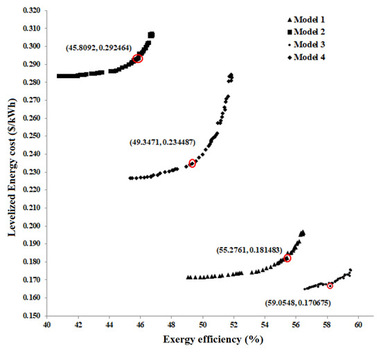
Figure 6.
The Pareto frontier solutions obtained by performing the optimization procedure for four predefined models with fixed mixing ratio of 0.5 for Pentane/R24fa working fluids.
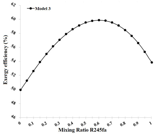
Figure 7.
The exergy efficiency of model 3 as a function of working fluid mixing ratio.
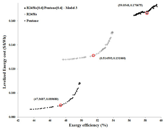
Figure 8.
The Pareto frontier solutions in the objective space for model 3 with three different working fluids, pure Pentane, pure R24fa and the combined Pentane [0.6]/R24fa [0.4].
Table 5.
The detail information about the best possible solutions for different working fluids.
To examine the model 3 with Pentane [0.6]/R24fa [0.4], its Pareto frontier solutions were illustrated in Figure 9.
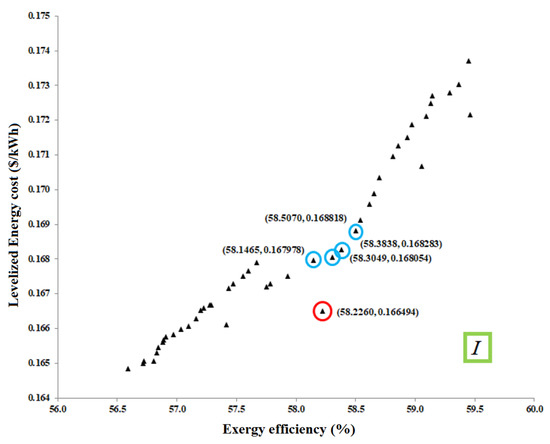
Figure 9.
The Pareto frontier solutions for model 3 with Pentane [0.6]/R24fa [0.4].
Points I in Figure 9, showed the ideal solution point in the objective space with the minimum possible levelized energy cost and maximum possible exergy efficiency. The five preferred solutions obtained with the TOPSIS are highlighted with blue and red cycles circumscribed the solution in Figure 9. The best possible solution is highlighted in the red cycle. The detail position of the points is presented in Table 6.
Table 6.
The five best solutions proposed by technique for the order of preference by similarity to ideal solution (TOPSIS) method for model 3 with Pentane [0.6]/R24fa [0.4].
The components’ exergo-economic specifications of the best possible solution selected in the last section are presented in Table 7. The relative cost difference, the entering and exiting cost, investment, and the exergo-economic coefficient for every component of the system are presented in Table 7.
Table 7.
The components’ exergo-economic specifications of the best possible solution.
Considering the values for every component, the most critical elements of the system can be determined. The greater value of for a component, the more decisive effect it has on the system. Thus, the turbine and the condenser consider as the most critical component of the system. The two highest exergo-economic coefficients f are allocated to the pump and the turbine, which determined the high investment cost of these components. The total exergo-economic coefficient of the system is 28.7518%, which means that 71.2482% of the system cost is allocated to the exergy destruction.
The irreversibility of the systems can justify the high exergy destruction of the condenser due to the inequalities between the received exergy by the clod flow and the released exergy by the warm flow. This might be the result of the heat exchange method used between the warm and cold flows, the heat exchange between the ambient environment and the exchanger, or the flow resistance. The same justification can be used for the evaporator.
Regarding the relative cost difference value r, the system components can be ordered as the pump, condenser, evaporator, turbine, and generator. As the relative cost difference value represented the component’s effectiveness on the cost increase, this ordering showed the component importance regarding the total system costs.
5. Conclusions
In the present study, using the average exergetic cost method and related equations, the parameters of ORC fed by the wasted heat of a sample power plant were calculated. A mixture fluid is used as the working fluid. In addition to the system efficiency criteria, the environmental efficiency of the fluids was considered in the working fluid determination. Regarding the use of mixture working fluid, four possible thermodynamic models have been investigated. Using the SPEA II algorithm, an exergo-economic optimization procedure was conducted on the ORC, and the optimum system was introduced regarding the working fluid mixing ratio effects.
The exergo-economic specifications of the different components of the system were examined in order to determine their relative role in the system efficiency. The turbine, condenser, and evaporator were found as the costliest components. They also were known to have the most decisive effects on system operation. The pump and turbine had the most prominent exergo-economic coefficients. Thus, reducing their purchasing cost and improving their efficiency would eventually improve the whole system. To optimize the pump functionality, one should avoid using it near its shut-off head point [29].
Reducing the exergy destruction and waste in the turbine is the most crucial factor in turbine efficiency. To achieve this, considering the turbine specification, the pressure drop, and the mass flow rate adaption is proposed. In the condenser and evaporator, the exergy wasted as the systems are irreversible. Insulation, choosing flow Discharge, and low pinch point temperature difference can lead to decreasing the exergy destruction.
As the system’s performance showed high sensitivity to the mixing composition. It is suggested to be added as an independent parameter for system optimization. Regarding the result of this study in ordering the importance of the components, one can improve the system efficiency by substituting the components for more expensive and more efficient components to achieve her/his desired system.
Author Contributions
Conceptualization, S.M., A.S.L., M.R.S., M.G.; methodology, S.M., R.D.; formal analysis, R.D., A.A.; investigation, S.M., A.A.; writing—original draft preparation, S.M., R.D., A.A.; writing—review and editing, A.S.L., M.R.S., M.G. All authors have read and agree to the published version of the manuscript.
Funding
This research received no external funding.
Conflicts of Interest
The authors declare no conflict of interest.
Nomenclature
| Product Exergy Flow Rate (w) | |
| Average Cost Per Unit of Fuel ($) | |
| Kth Component Product Exergy Flow Rate (w) | |
| Kth Component Exergy Efficiency | |
| Entering Rate of Exergy Transfer (w) | |
| Average Costs per Unit of Entering Exergy ($/GJ) | |
| Exiting Rate of Exergy Transfer (w) | |
| Average Costs per Unit of Exiting Exergy ($/GJ) | |
| Power (w) | |
| Average Costs per Unit of power ($/w) | |
| Exergy Transfer Rate associated with Heat Transfer (w) | |
| Average Costs per Unit of Exergy Associated with heat transfer ($/GJ) | |
| Fuel Cost Rate ($/h) | |
| Capital Recovery Factor | |
| Coefficient of Operating & Maintenance Costs | |
| Kth Component Investment Cost ($) | |
| Inflation Rate | |
| Number of System Operating Years | |
| Relative Cost Difference for Kth Component | |
| Exergoeconomic Factor | |
| Kth Component Purchase Cost ($) | |
| Number of System Operation Hours | |
| Exergy Loss Cost Rate ($/h) | |
| Exergy Destruction Cost Rate ($/h) | |
| CI | Capital Investment |
| OM | Operation and Maintenance |
References
- Li, Y.-R.; Du, M.-T.; Wu, S.-Y.; Peng, L.; Liu, C. Exergoeconomic analysis and optimization of a condenser for a binary mixture of vapors in organic Rankine cycle. Energy 2012, 40, 341–347. [Google Scholar] [CrossRef]
- El-Emam, R.S.; Dincer, I. Exergy and exergoeconomic analyses and optimization of geothermal organic Rankine cycle. Appl. Therm. Eng. 2013, 59, 435–444. [Google Scholar] [CrossRef]
- Khaljani, M.; Saray, R.K.; Bahlouli, K. Comprehensive analysis of energy, exergy and exergo-economic of cogeneration of heat and power in a combined gas turbine and organic Rankine cycle. Energy Convers. Manag. 2015, 97, 154–165. [Google Scholar] [CrossRef]
- Yari, M.; Mehr, A.S.; Zare, V.; Mahmoudi, S.M.S.; Rosen, M.A. Exergoeconomic comparison of TLC (trilateral Rankine cycle), ORC (organic Rankine cycle) and Kalina cycle using a low grade heat source. Energy 2015, 83, 712–722. [Google Scholar] [CrossRef]
- Yang, M.-H.; Yeh, R.-H. Thermo-economic optimization of an organic Rankine cycle system for large marine diesel engine waste heat recovery. Energy 2015, 82, 256–268. [Google Scholar] [CrossRef]
- Sadeghi, M.; Nemati, A.; Yari, M. Thermodynamic analysis and multi-objective optimization of various ORC (organic Rankine cycle) configurations using zeotropic mixtures. Energy 2016, 109, 791–802. [Google Scholar] [CrossRef]
- Ustaoglu, A.; Alptekin, M.; Akay, M.E. Thermal and exergetic approach to wet type rotary kiln process and evaluation of waste heat powered ORC (Organic Rankine Cycle). Appl. Therm. Eng. 2017, 112, 281–295. [Google Scholar] [CrossRef]
- Scardigno, D.; Fanelli, E.; Viggiano, A.; Braccio, G.; Magi, V. Dataset of working conditions and thermo-economic performances for hybrid organic Rankine plants fed by solar and low-grade energy sources. Data Br. 2016, 7, 648–653. [Google Scholar] [CrossRef]
- Wang, Y.Z.; Zhao, J.; Wang, Y.; An, Q.S. Multi-objective optimization and grey relational analysis on configurations of organic Rankine cycle. Appl. Therm. Eng. 2017, 114, 1355–1363. [Google Scholar] [CrossRef]
- Nazari, N.; Heidarnejad, P.; Porkhial, S. Multi-objective optimization of a combined steam-organic Rankine cycle based on exergy and exergo-economic analysis for waste heat recovery application. Energy Convers. Manag. 2016, 127, 366–379. [Google Scholar] [CrossRef]
- Zhou, Y.; Zhang, F.; Yu, L. Performance analysis of the partial evaporating organic Rankine cycle (PEORC) using zeotropic mixtures. Energy Convers. Manag. 2016, 129, 89–99. [Google Scholar] [CrossRef]
- Wang, J.; Xu, P.; Li, T.; Zhu, J. Performance enhancement of organic Rankine cycle with two-stage evaporation using energy and exergy analyses. Geothermics 2017, 65, 126–134. [Google Scholar] [CrossRef]
- Bufi, E.A.; Camporeale, S.M.; Cinnella, P. Robust optimization of an Organic Rankine Cycle for heavy duty engine waste heat recovery. Energy Procedia 2017, 129, 66–73. [Google Scholar] [CrossRef]
- Scardigno, D.; Fanelli, E.; Viggiano, A.; Braccio, G.; Magi, V. A genetic optimization of a hybrid organic Rankine plant for solar and low-grade energy sources. Energy 2015, 91, 807–815. [Google Scholar] [CrossRef]
- Zitzler, E.; Laumanns, M.; Thiele, L. SPEA2: Improving the Strength Pareto Evolutionary Algorithm; TIK-Report 103; Computer Engineering and Networks Laboratory: Zurich, Switzerland, 2001. [Google Scholar]
- Hwang, C.-L.; Yoon, K. Methods for multiple attribute decision making. In Multiple Attribute Decision Making; Springer: Berlin/Heidelberg, Germany, 1981; pp. 58–191. [Google Scholar]
- Feng, Y.; Hung, T.; Greg, K.; Zhang, Y.; Li, B.; Yang, J. Thermoeconomic comparison between pure and mixture working fluids of organic Rankine cycles (ORCs) for low temperature waste heat recovery. Energy Convers. Manag. 2015, 106, 859–872. [Google Scholar] [CrossRef]
- Bejan, A.; Tsatsaronis, G.; Moran, M.J. Thermal Design and Optimization; John Wiley & Sons: Hoboken, NJ, USA, 1995. [Google Scholar]
- Moran, M.J.; Shapiro, H.N.; Boettner, D.D.; Bailey, M.B. Fundamentals of Engineering Thermodynamics; John Wiley & Sons: Hoboken, NJ, USA, 2010. [Google Scholar]
- Tsatsaronis, G.; Pisa, J. Exergoeconomic evaluation and optimization of energy systems—Application to the CGAM problem. Energy 1994, 19, 287–321. [Google Scholar] [CrossRef]
- Quoilin, S.; Declaye, S.; Tchanche, B.F.; Lemort, V. Thermo-economic optimization of waste heat recovery Organic Rankine Cycles. Appl. Therm. Eng. 2011, 31, 2885–2893. [Google Scholar] [CrossRef]
- Feng, Y.; Hung, T.; Zhang, Y.; Li, B.; Yang, J.; Shi, Y. Performance comparison of low-grade ORCs (organic Rankine cycles) using R245fa, pentane and their mixtures based on the thermoeconomic multi-objective optimization and decision makings. Energy 2015, 93, 2018–2029. [Google Scholar] [CrossRef]
- Baasel, W.D.; von Matt, L. Preliminary Chemical Engineering Plant Design; Elsevier: New York, NY, USA, 1976. [Google Scholar]
- Lozowski, D.; Ondrey, G.; Jenkins, S.; Bailey, M.P. Chemical engineering plant cost index (CEPCI). Chem. Eng. 2012, 119, 84. [Google Scholar]
- Li, Y.-R.; Du, M.-T.; Wu, C.-M.; Wu, S.-Y.; Liu, C.; Xu, J.-L. Economical evaluation and optimization of subcritical organic Rankine cycle based on temperature matching analysis. Energy 2014, 68, 238–247. [Google Scholar] [CrossRef]
- Jaszkiewicz, A. On the performance of multiple-objective genetic local search on the 0/1 knapsack problem-a comparative experiment. IEEE Trans. Evol. Comput. 2002, 6, 402–412. [Google Scholar] [CrossRef]
- Zitzler, E.; Thiele, L. Multiobjective evolutionary algorithms: A comparative case study and the strength Pareto approach. IEEE Trans. Evol. Comput. 1999, 3, 257–271. [Google Scholar] [CrossRef]
- Kolahi, M.; Yari, M.; Mahmoudi, S.M.S.; Mohammadkhani, F. Thermodynamic and economic performance improvement of ORCs through using zeotropic mixtures: Case of waste heat recovery in an offshore platform. Case Stud. Therm. Eng. 2016, 8, 51–70. [Google Scholar] [CrossRef]
- Gulich, J.F. Centrifugal Pumps; Springer: Berlin/Heidelberg, Germany, 2008. [Google Scholar]


© 2020 by the authors. Licensee MDPI, Basel, Switzerland. This article is an open access article distributed under the terms and conditions of the Creative Commons Attribution (CC BY) license (http://creativecommons.org/licenses/by/4.0/).