Abstract
Industrial waste heat recovery is an attractive option having the simultaneous benefits of reducing energy costs as well as carbon emissions. In this context, thermal energy storage can be used along with an optimal operation strategy like model predictive control (MPC) to realize significant energy savings. However, conventional control methods offer little robustness against uncertainty in terms of daily operation, where supply and demand of energy in the cluster can vary significantly from their predicted profiles. A major concern is that ignoring the uncertainties in the system may lead to the system violating critical constraints that affect the quality of the end-product of the participating processes. To this end, we present a method to make optimal energy storage and discharge decisions, while rigorously handling this uncertainty. We employ multivariate data analysis on historical industrial data to implement a multistage nonlinear MPC scheme based on a scenario-tree formulation, where the economic objective is to minimize energy costs. Principal component analysis (PCA) is used to detect outliers in the industrial data on heat profiles, and to select appropriate scenarios for building the scenario-tree in the multistage MPC formulation. The results show that this data-driven robust MPC approach is successfully able to keep the system from violating any operating constraints. The solutions obtained are not overly conservative, even in the presence of significant deviations between the predicted and actual heat profiles. This leads to an energy-efficient utilization of the storage unit, benefiting all the stakeholders involved in heat-exchange in the cluster.
1. Introduction
The International Energy Agency estimates that the industrial sector accounts for more almost two-fifths of the global energy consumption [1]. As such, this sector is responsible for releasing large quantities of industrial waste heat to the environment—via cooling media, exhaust gases, and hot equipment surfaces, among others. This is especially true for chemical, minerals and metals, pulp and paper, and the food industries [2]. Recovering, storing, and reusing this surplus heat when required is a means of improving industrial energy efficiency and lowering its overall environmental impact. Moreover, waste heat recovery presents a low-cost energy resource with the potential to realize significant energy savings, improving the competitiveness of the sector.
According to [3], industrial symbiosis occurs when multiple process plants are located within the same geographical area, facilitating by-product reuse, utilities and infrastructure sharing, and a joint provision for shared services. Surplus heat recovery is an especially attractive proposition for such industrial clusters since it presents an opportunity for flexible energy exchange within the cluster, with plants representing both sources and sinks of surplus heat. Today, recovered high-grade heat is mostly reused within the process itself in order to reduce exergy losses, but low-grade surplus heat below 200 °C provides recovery potential for external energy exchange [4]. Such low-grade heat integration is thus highly beneficial for energy exchange in industrial clusters, since participating plants can fulfill their low-grade heat demands from within the cluster itself.
For optimal use of energy, two main aspects must be considered: (1) Design of the process and its infrastructure; and (2) How to optimally operate the system to maximize energy recovery. For example, in [5], optimal location of the intermediate-fluid circuits was determined for heat integration across multiple plants to maximize savings. Some studies have focused specifically on design optimization in industrial clusters [6,7,8,9]. However, even for plants with a well-designed surplus heat recovery system, there may be further operational and control challenges to deal with. A prominent operational challenge for surplus heat exchange between multiple plants is the temporal decoupling between the availability of surplus heat and its demand [10]. From the various available technologies [11], thermal energy storage (TES) is a viable option to handle this issue. Surplus heat is supplied to, and extracted from, a TES unit at different temperatures, allowing for a diverse set of plants to participate in the energy exchange. TES units offer operating flexibility to heat recovery by creating a buffer between the supply and demand of surplus heat, thereby reducing peak energy requirements. With TES, however, the dynamic operational aspects become extremely important. Optimal operation and control of TES units has been studied previously within different application areas. For instance, optimal operation of TES units in buildings for reducing peak loads was considered by [12]. In [13,14], model predictive control (MPC) is implemented on a TES system for energy-efficient buildings. Another application of MPC on a TES system for multi-energy district boilers is investigated in [15]. Classical control techniques like the proportional-integral-derivative (PID) control have also been investigated, for instance in TES for concentrated solar polar [16]. An optimal control scheme was proposed by [17] for surplus heat exchange using TES in industrial clusters. A review of various types of TES and their applications can be found in [18,19], whereas a review of optimization and control for TES systems is given in [20].
A TES unit within an industrial cluster setting presents a unique challenge from an operator’s perspective, in that there are various system uncertainties to contend with. In [21], it is noted that supply of low-grade surplus heat is usually unstable because of temperature fluctuations in the processes producing it. Similarly, there is volatility in consumer-side heat demands and process temperatures. These uncertainties in the supply and demand profiles of surplus heat affect efficient utilization of the TES unit. Additionally, daily variability in the electricity prices can directly influence the operating costs, since electricity from the grid is often used for peak heating. Disregarding these uncertainties in the system can lead to control solutions that are not only suboptimal, but also infeasible. The plant–model mismatch that arises due to these uncertainties may result in control solutions that cause critical constraint violations. In an industrial cluster, this may translate to larger heat-acquisition costs to satisfy consumer demands, leading to high carbon emissions if fossil fuel-based peak heating is involved. Operating constraints relating to safety or process specifications may also be violated. Such constraint violations usually come with a significant economic penalty, and so may not be acceptable to the stakeholders in the industrial cluster.
To achieve robust operation against uncertainty, the multistage nonlinear MPC proposed by [22] can be employed. Here, the uncertainty is modeled in terms of discrete scenarios of operation, evolving in the form of a “scenario-tree”. The scenario-tree gives a measure of how future control inputs can take recourse action to negate the effect of future uncertainties, since these scenarios are explicitly modeled. This notion of feedback is what makes the multistage MPC less conservative than other robust MPC methods like the min-max MPC [23]. However, a limitation of this approach is that the problem size increases exponentially an with increasing number of considered scenarios. For computational efficiency, it is important to capture maximum uncertainty information with fewer scenarios.
In this context, the availability of historical data from industrial processes motivates the need for data-driven approaches to scenario selection in multistage MPC. Industrial data is particularly useful for heat integration processes, since the heat supply and demand profiles often exhibit correlations. Principal component analysis (PCA) is a popular multivariate data-analysis method that can be used to identify correlations in such datasets. By identifying correlations, PCA is able to explain the uncertainty data in fewer dimensions. This means it can be effectively leveraged to choose fewer scenarios without losing uncertainty information, leading to a compact scenario tree for multistage MPC. Apart from dimensionality reduction, PCA can be used in data pre-processing to detect outliers. These represent instances where the system was either sampled wrongly or was not in normal operation. Statistically, outliers are considered to not be a part of the general sampling population, and are excluded from our analysis to avoid unnecessary conservativeness in scenario selection.
Although a control method like the standard MPC offers a limited degree of robustness against process disturbances [24], it does not explicitly account for uncertainties in the system. In this paper, we argue that for optimally operating a TES unit in an industrial cluster, uncertainty in heat supply and demand must be taken into account rigorously. To this end, we implement the scenario-based multistage MPC method on an industrial cluster model. We further show that the inherent correlations present in the supply and demand profiles can be exploited using the data-driven PCA approach, and that these can be used to quantify the uncertainty in the multistage MPC framework. We demonstrate that in comparison to a standard MPC formulation where uncertainties are not modeled, the proposed framework leads to an efficient utilization of the TES unit by avoiding violations of critical operating constraints specified by the stakeholders in the industrial cluster.
2. Methods
2.1. System Modeling
Figure 1 illustrates the topology of an industrial cluster with suppliers and consumers of heat, along with a TES as buffer. The TES unit is considered to be a hot water tank.
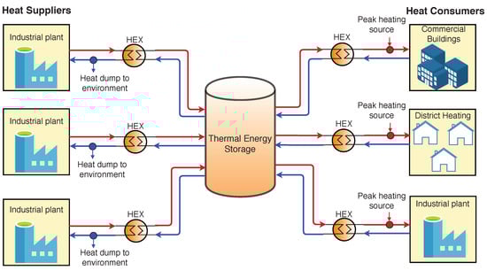
Figure 1.
Topology of an industrial cluster with multiple energy suppliers and consumers, with a thermal energy storage (TES) as buffer. The red lines represent the hot streams and the blue ones cold streams.
The supplier plants are sources of energy, supplying excess heat to the TES. On the other hand, the consumer plants are heat sinks, extracting energy from the TES to fulfill their energy demands. The heat exchange between the supplier/consumer plants and the TES happens with the help of heat exchangers, with hot water being the energy carrier. The temperatures of the process streams in the supplier and consumer plants drive the heat transfer.
In cases of high volatility with sharp fluctuations in heat demand on the consumer side, it may happen that the energy from the TES is not enough to satisfy any extra demand. A common practice for such an extra-demand scenario is to purchase electricity externally from the market, or to burn fossil fuels using boilers, to heat up the required process streams. Not only are these peak heating sources of energy expensive, significantly increasing the operating costs in the cluster, but they also lead to higher carbon emissions. The source of surplus heat in the suppliers is assumed to be the cooling of certain batch processes. As such, the suppliers can dump heat to the environment to meet their cooling demands.
In this paper, we focus on modeling the dynamics of the heat exchange between the TES, and one pair of supplier and consumer plants. This involves the energy balances over the heat exchangers and over the TES. The heat exchangers are considered to have countercurrent flow, and are discretized in space into a series of cells. Each cell of the heat exchanger is assumed to be well mixed, such that the temperature within the cell volume is the same as the exit temperature. The carrier fluid is assumed to be incompressible and has a constant heat capacity. Further, we consider that the supplier and consumer plants are close enough to each other such that the heat losses in the pipes due to time delays are assumed to be negligible.
The incoming surplus heat from the supplier is denoted as . This heat has to be delivered through the supply-side heat exchanger to the tank. The temperature at which this heat is supplied is denoted by and the return temperature (after exiting the heat exchanger) is denoted by . On the return stream, there is a provision to dump heat so as to reduce the return temperature to a desired level, denoted by . The temperatures on the hot and cold sides of the heat exchanger are denoted by and , where is the cell index of the heat exchanger. The volumetric flow rates on the hot and cold sides of the supplier-side heat exchanger are denoted by and . The supplier-side temperatures can be collected into vectors . Similarly, we denote the volumetric flow rates . Formulating the energy balances on the supplier side results in the following:
where is the vector-valued function describing the ordinary differential equations (ODE) system. is the heat supplied to the TES, and can be calculated as the heat transfer from the hot to cold side of the heat exchanger (since heat loss in the pipes is negligible).
where is the heat-transfer conductance of the heat exchangers.
On the consumer side, the demanded heat flow rate is . Analogous to the supplier-side temperatures, we denote the vector for consumer-side temperatures , and the vector for volumetric flow rates . On the consumer side, there is a provision to heat up the return stream using the expensive peak heating to satisfy required demand, denoted by . The resulting energy balances are:
where is the vector-valued function describing the ODEs on the consumer side, and is the heat extracted from the TES.
The details of the vector-valued functions and are explained in Appendix A.
Typically, a large hot water tank will have a temperature gradient along its height leading to different densities at the top and the bottom of the tank. In this work, however, modeling of such thermal stratification is not considered. Instead, the tank is assumed to have uniform mixing throughout its volume, such that the temperature within the tank is same as the tank outlet temperature, denoted by . Since the temperature ranges considered in this paper are below the boiling temperature of water, we assume an unpressurized tank. The tank volume is , the density and the specific heat capacity of water are denoted by and respectively. The resulting TES energy balance is:
where is the heat lost by the tank to the surroundings.
where is the heat-loss conductance of the tank, and is the ambient temperature. Note that the volumetric flow rates into and out of the tank are always equal, so the fluid volume inside the tank always remains constant (see Figure A1). The initial conditions for the temperatures can be stated as:
where , , and are the initial values for each of the temperatures.
2.2. Dynamic Optimization of TES
Dynamic operational optimization of the energy storage requires a central cluster operator to apply optimal control inputs to the system such that the heating and cooling requirements of the plants in the industry cluster is satisfied. Table 1 shows the states, inputs, and uncertainties in the system. The volumetric flow rates on the supplier side, , are considered to be fixed, and are not degrees of freedom in the system. The operator should thus determine how much heat to dump on the supplier side, , and how much heat to acquire through the peak heating sources, , on the consumer side. Additionally, the operator must determine how much heat can be extracted from the TES by adjusting the volumetric flow rates through the consumer-side valves, . Determining optimal values of the inputs requires prediction of the uncertainty in the system, which pertains to the heat supply and demand, and . The developed model estimates the future evolution of temperatures in the system for given inputs using the predicted values of heat supply and demand.

Table 1.
System states, inputs, and uncertainties.
There are various operating constraints to deal with within the heat exchange framework. These may relate to physical limitations on certain variables, safety considerations, or some performance criteria. Since the tank is considered to be unpressurized, its temperature is upper bounded with so as to prevent boiling. Further, there is a lower bound on the tank temperature, , in order to prevent growth of bacteria in the tank. Similar bounds are applicable to the other temperatures. For instance, process specifications may mandate that the return temperatures (on either side) are below a certain maximum value.
The various volumetric flow rates are also constrained between certain values. These values may represent the physical limit of the flow rate (e.g., 0% and 100% valve openings). Also worth noting is that a very low flow rate may lead to fast fouling of the heat exchanger, necessitating a lower bound. Similarly, there are limits on the operation of the heat pumps that are used for heat dumping or peak heating.
The economic objective for the operator is to minimize the use of expensive peak heating sources in the industrial cluster. This can be formulated as the objective function:
The integral represents the total peak heating during the operating period of to . Objective (16) is an cost function, which assists in getting sparse solutions [25]. It also ensures that peak heating is only used in cases where the heat demands cannot be fully met by the TES. With a purely economic objective, the idea is for the cluster operator to primarily give directives on how much heat to dump to the surroundings and/or how much peak heating to use, at every hour. We assume that there is a lower regulatory level (e.g., PID control) to handle other process disturbances on a faster time scale—e.g., in temperatures, mass flows, etc.
Remark 1.
We have added regularization terms to the linear objective (16) in our simulations to avoid ill-conditioned singular control problems (see Chapter 10 of [26]). These terms are quadratic costs associated with the other control inputs and , weighted with some positive penalty parameters 1. This is similar to the objective function formulation used in [17].
Finally, the dynamic optimization problem can be described as having to minimize the objective function (16), subject to the system dynamics represented by the model Equations (1)–(9) and the operating constraints (10)–(12) and (13)–(15). Equation (A9) in Appendix B shows the complete formulation of the dynamic optimization problem.
2.3. Standard and Multistage Model Predictive Control
The problem (A9) has continuous-time dynamics and is thus infinite-dimensional. This problem is converted into a finite-dimensional nonlinear program (NLP) by discretizing the equations into finite elements.The inputs and uncertain parameters are also considered discretized. In the standard MPC framework, this discretized dynamic optimization problem can be stated compactly as follows:
where N is the length of the prediction horizon of the dynamic optimization problem (each time step indexed by the subscript j). The states and inputs for the jth time step are denoted by and respectively. Equation (17a) represents the minimization of cost Equation (17b) show the initial conditions, with being the vector of starting points for each of the states. Equation (17c) represents the mathematical model of the nonlinear dynamic system, described by the vector of state equations . Equation (17d) represents the system constraints, denoted by . Note that the uncertain parameters are not explicitly modeled in problem (17).
To account for the mismatch between the model and the real system, state feedback information is incorporated by repeatedly solving problem (17). After every time step, problem (17) is solved with updated state information, and with a receding prediction horizon. The updated state information typically comes from a state observer that uses input-output data of the controlled system to compute the new states. However, observers are not needed in cases where the states are directly measurable—like temperatures. The reader is referred to [27] for a comprehensive discussion on MPC.
Remark 2.
In conventional MPC implementations, terminal state constraints are added separately to ensure stability and recursive feasibility of the MPC. However, stable performance is often observed in the absence of such terminal constraints (see [28], for example). In our study, the fluid volume in the TES never empties as it is always constant owing to equal flows in and out of the TES. The TES model dynamics also implicitly ensure that the TES temperature is always between the supplier (upper bound) and consumer (lower bound) process temperatures during operation. This prevents the energy in the TES from depleting all at once at the end of the prediction horizon. When the energy in the TES is sufficiently depleted (i.e., when the across the consumer-side heat exchanger is too small to facilitate heat transfer), the peak heating on the consumer side takes over. As such, the system tends to be stable in terms of energy in the TES because, at worst, the consumer can use peak heating to satisfy any excess demand without having to destabilize the TES. Moreover, since we consider a long enough prediction horizon, we avoid such “at worst" suboptimal solutions.
The typical standard MPC strategy used for optimal operation for the industrial cluster case study is illustrated in Figure 2. However, this implementation does not explicitly account for the uncertainty in the heat supply and demand in the optimizer. System–model mismatch arising from these uncertain parameters may cause the optimizer to suggest control actions that cause the system to violate critical operating or safety constraints. Another possible consequence is that the resulting optimization problem might simply be infeasible. This uncertainty can be modeled in the form of discrete realizations of the supplied and demanded heat flow rates. Each scenario represents a unique combination of specific realizations of the uncertain parameters: and . The multistage MPC approach, described next, is used to deal with such a robust control problem with scenario-based uncertainty.
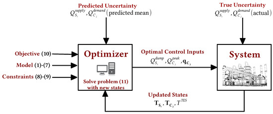
Figure 2.
Standard model predictive control scheme with data flow between optimizer and the system.
Using notation analogous to problem (17), the scenario-based multistage optimal control problem is formulated as follows:
where M is the total number of scenarios (each scenario indexed with the subscript i). The uncertain parameters for the ith scenario are denoted by and is the weight assigned to the ith scenario. The scenario weights may be based on some underlying probability distribution if such information is availble. In this paper, we consider equal weights for all scenarios.
Equation (18e) represents the non-anticipativity constraints. The non-anticipativity constraints enforce that all control inputs that branch at the same node are equal. This is because, in real applications, the uncertainty is realized only after the control input is applied. In other words, one cannot anticipate how the scenario-tree is going to branch out at a node before a decision is taken at that node. The reader is referred to [29] for details on the construction of the non-anticipativity matrix .
Branching of scenarios at every time step of the prediction horizon leads to rapid growth of the scenario-tree. To curb this, the uncertainty can be assumed to be constant after a certain point in the prediction horizon in order to ease the computational effort [30]. This point corresponds to the so-called robust horizon of the problem, with a length . The scenario-tree evolution showing the prediction horizon and the robust horizon is illustrated in Figure 3. Therefore, for D discrete realizations of the uncertainty, there are scenarios. The NLP (18) is solved in a closed-loop, receding-horizon fashion to implement the multistage MPC. For the industrial cluster problem, the multistage MPC strategy is shown in Figure 4. This implementation is similar to that of the standard MPC, but with the scenario-tree being an additional input to the optimizer to model the uncertainty in heat supply and demand.
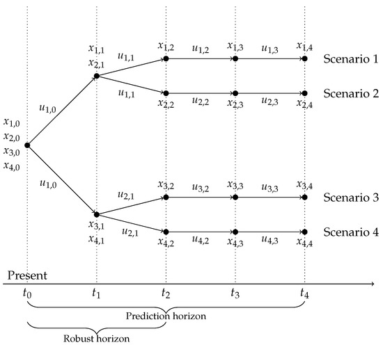
Figure 3.
Illustration of a scenario-tree with realizations of uncertainty. The prediction horizon and the robust horizon .
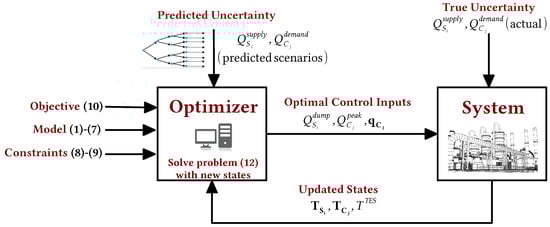
Figure 4.
Multistage model predictive control scheme with data flow between optimizer and plant.
2.4. Data-Driven Selection of Scenarios in Multistage MPC
The scenarios selected in multistage MPC should be representative of the uncertainty in the system. Conventionally, uncertain parameters are described using probability distribution functions (PDFs), which may be statistically derived from historical measurement data. In scenario-based approaches to stochastic optimization, these PDFs are then discretized to generate scenarios. For easier computation, it is important to sufficiently describe the parametric uncertainty with few scenarios, since the scenario-tree grows exponentially with increasing number of scenarios. As such, the discretization of the PDF can be chosen according to the required confidence interval. In [31,32], a data-driven approach is proposed for scenario selection when the uncertain parameters exhibit interdependencies. Such correlations in the uncertain parameters can be exploited using multivariate data-analysis techniques like PCA, which we employ in this work.
The PCA is an orthogonal linear transformation of an existing data set into a new coordinate system, where the new axes are called principal components (see [33], for example). The first principal component aligns in the direction of maximum variance in the data, and subsequent components explain the remaining data variance in decreasing order. Consider a scaled data matrix , where is the number of observations and is number of the uncertain parameters. The PCA procedure on results in a transformed data matrix , with , according to . Here, is the projection matrix, where each column represents a principal component. The columns of contain the coefficients, called loadings, that project the original data point to the new coordinate system of principal components. The new data matrix is called the scores matrix. The score of a data point along a principal component represents the distance of that data point from the mean along the direction of that principal component.
We select scenarios corresponding to the maximum and minimum scores along the dominant principal component that explains the variations in the data sufficiently. Figure 5 shows scenarios marked by red “X”s selected along the dominant principal component. In addition, we also select a scenario representing the mean value in each dimension. It can be seen that the chosen scenarios encompass most of the parametric variation in the data shown in Figure 5, without any significant loss in explained variability. Using fewer scenarios makes the size of resulting multistage MPC problem significantly smaller.
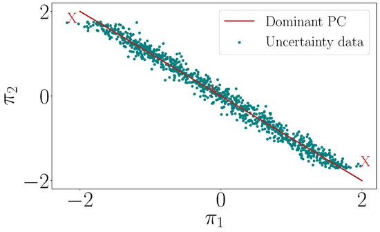
Figure 5.
Selected scenarios, marked by ‘X’, correspond to the maximum and minimum scores along the first principal component, along with the mean.
3. Case Study: Data Description and Analysis
We consider a case study with one supplier and one consumer of heat, exchanging heat via a TES tank. The values of the various system parameters are given in Table 2.
Table 2.
System parameters.
A tank volume of is considered. This approximately corresponds to a cylindrical tank with a height of 10 m and a diameter of 11 m. The heat losses in heat exchangers, and in the pipes carrying the hot water, are considered to be negligible. The operating bounds on the various system variables are given in Table 3.
Table 3.
Operating bounds.
The heat supply and demand data used in this case study is based on the 2017 data from Mo Fjernvarme, a district heating company which is part of the Mo Industrial Park in northern Norway. The surplus heat in Mo Fjernvarme is sourced from a smelting plant within the industrial park in form of flue gases. The demand, on the other hand, comes from the town of Mo i Rana and from within the industrial park itself. For simplicity, we do not model the various processes within Mo Industrial Park in this work. As such, the models that describe our case study are not directly related to the industry park layout or processes. We instead focus on the overall heat supply and demand data from the industry park for data analysis, along with the general model developed in Section 2.1, to demonstrate the effectiveness of our proposed approach.
The hourly heat supply and demand for 2017 is shown in Figure 6. For the spring, summer, and fall months of April to November, it can be seen that the demand is lower. However, for the winter months of January–March and December, there is large variation in the demand compared to a relatively smaller variation in supply. Since optimal operation is considered on a daily basis, a TES unit is not relevant for periods when supply is always higher, since the demand can be completely satisfied by the supplied heat. However, for the winter months, an optimal operation strategy would allow for making TES storage and discharge decisions in order to reduce the peak heating. Moreover, for diurnal thermal storage there must be a period in the day at which supply is greater than demand. Figure 7 shows the aggregated heat supply and demand for each month of 2017.
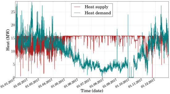
Figure 6.
The hourly supplied and demanded heat flow rates for 2017.
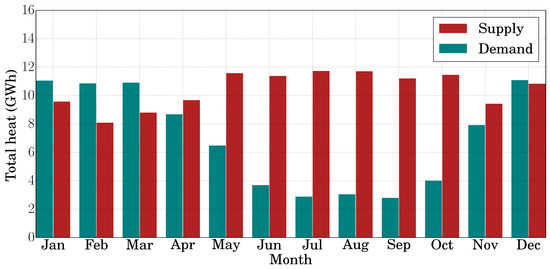
Figure 7.
The total supplied and demanded heat for each month of 2017.
We analyzed the demand and supply data the winter months of January–March and December to detect any outliers. For a total of 121 winter days with hourly variation in heat flows, PCA was performed separately in both sets of supply and demand data. Our analysis shows that there were many outliers in the data during the month of December, and hence this month was discarded (see Appendix C for more details on outlier detection). Of the remaining winter months, January shows the least difference between the total supplied heat and the total heat demand, making it a suitable candidate to inspect daily storage. Hence, we focus on the month of January in this work.
Since hourly heat data is available, the January data includes 31 sample points (for 31 days), corresponding to each of the 24 h of the day. However, our analysis in Figure A2 shows that the 2nd, 3rd, 4th, 5th, and the 13th days of the month are outliers in terms of either the heat supply or demand. Hence, these are excluded from the analysis. The scatter plot of the data points for each of the 24 h is shown in Figure 8. For most of the day, a linear correlation can be seen for the heat supply and demand. The exceptions are the morning hours of 8–10 a.m., and the afternoon hours of 3–5 p.m. These are the peak demand hours, as can be expected of a district heating system. The supply and demand data for these hours are thus not linearly correlated to each other. Figure 9 shows the mean hourly demand trend averaged over the winter months of January–March and December. It is evident that 8–10 a.m. and 3–5 p.m. are the expected peak heating hours.
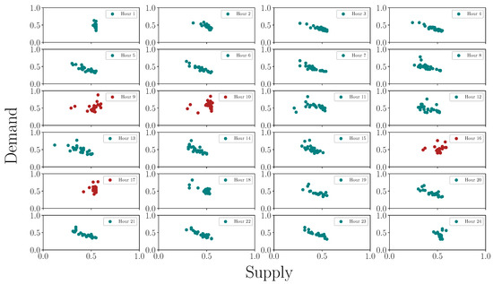
Figure 8.
Hourly scatter plot of heat supply and demand (normalized) in January. The plots in blue show a linear trend in the data. The plots in red correspond to the peak demand hours, and do not show the linear correlation.
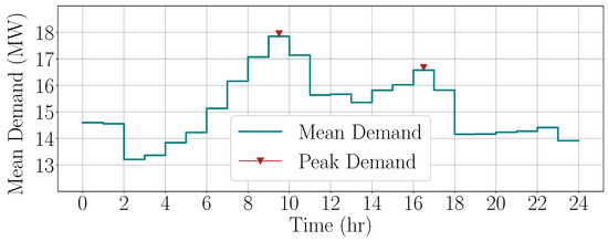
Figure 9.
Mean hourly demand data for winter months (January-March and December) in 2017 showing expected peak demand hours between 8–10 a.m. and 3–5 p.m.
The aim is to apply the optimal control strategy for operation during a typical January 2018 day, based on the available January 2017 data shown in Figure 8. Applying standard or multistage MPC as described in Section 2.3 requires a prediction of the heat supply and demand across the prediction horizon, which is taken to be 24 h. These values are taken to be the means of the data corresponding to each of the scatter plots in Figure 8. Additionally, the multistage MPC also requires scenario selection for each hour of operation. This scenario selection can be done by performing PCA on the corresponding scatter plots in Figure 8, as explained in Section 2.4. For the non-peak demand hours, since there is a strong linear correlation between the supply and demand, the scenarios are chosen only along the dominant principal component. This implies a total of 3 scenarios, corresponding to the minimum and maximum scores, along with the mean value. For the peak hours of 8–10 a.m. and 3–5 p.m., the correlation is not strong enough, and thus the scenarios are chosen along the first two principal components to more accurately encompass the uncertainty. The number of scenarios is 5, corresponding to the extreme scores along the two principal components, along with the mean.
4. Results and Discussion
The infinite-dimensional problem (A9) is converted into a finite-dimensional NLP by using third-order Radau collocation to approximate the state equations. The inputs and the uncertain parameters are discretized into finite elements, but are considered to be piecewise constant within each element. The reader is referred to Chapter 10 of [26] for more on the collocation-based discretization method. We consider a prediction horizon of h. The finite-dimensional NLP is formulated using 24 finite elements, implying that control action is taken every hour. This also implies that the uncertain parameters are assumed to evolve on an hourly basis, as is also the case from the industrial data.
The scenarios representing the uncertainty are chosen according to PCA from their respective January 2017 data sets. As explained before, we have discrete realizations of the uncertainty for every stage of the multistage MPC problem, in case of the non-peak demand hours. Similarly, we have discrete realizations for the peak hours. We assume a robust horizon of in this study, giving us either 3 or 5 total scenarios in the multistage MPC problem, depending on the hour of operation. Further, we consider equal weights for all scenarios.
To evaluate the effectiveness of the multistage MPC strategy for this case study, we compare it with a standard MPC formulation where no uncertainty is considered. To simulate the “true” plant data, we use the same system model as that in the NLP, but the heat supply and demand data from a typical day in January 2018. For comparison, identical data representing the true values of heat supply and heat demand is used in the plant simulation, for both the standard and multistage MPC methods.
An important point to note is that we only consider the application of both the MPC strategies during dynamic operation of the TES, and not during edge-cases like when the TES is empty at the start. The initial conditions of the system are obtained by solving the steady-state problem of the system for some given heat supply and demand. To begin with an empty TES would be equivalent to a start-up phase where all the supplied heat goes to heating up the tank, and all the demanded heat is fulfilled via peak heating. In this case, there are not enough degrees of freedom to improve performance or robustness via MPC, especially over a shorter horizon. The advantage of using MPC is thus not obvious in this case.
The NLPs (17) and (18) are modeled using the software JuMP [34] (version 0.18.5), within the framework of the Julia [35] (version 0.6.2). The solver used within this framework is Ipopt [36] (version 3.12.8), which uses interior-point algorithms to solve the NLPs. The MA27 [37] linear solver is used within Ipopt. It must be noted that Ipopt is not a global optimization solver. This implies that for nonconvex problems like the one considered in this paper, Ipopt can guarantee local, but not global, optimality.
4.1. Storage vs. No Storage
We begin by demonstrating the advantage and the economic benefit of using the TES as a buffer, as opposed to direct heat exchange between the suppliers and consumers. The modeling of the system without storage considers a single heat exchanger that is used to directly couple the supplier and the consumer. Figure 10 shows the results of a standard MPC formulation applied to both cases—with and without storage. For the sake of this comparison, no plant–model mismatch is considered, implying perfect prediction of supply and demand by the cluster operator. Further, the initial temperature of the tank is 70.63 °C.
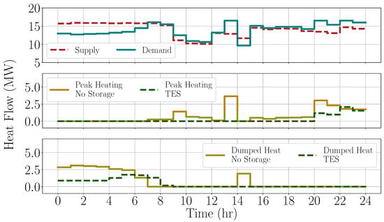
Figure 10.
The heat supply and demand across 24 h; and the heat dumping and peak heating as obtained by standard MPC applied to the cases with and without thermal storage.
In the case with no storage, the extent of peak heating and dumping is solely determined by the operating bounds on the system variables. As such, the predictive ability of MPC does not provide any added benefit for operation. When the supply exceeds the demand, the excess heat is dumped and when the demand exceeds the supply, the deficit heat is acquired through peak-heating—subject to the operating constraints. On the other hand, using TES significantly reduces the heat dumping as well as peak heating. During periods of low demand, the excess heat is used to charge up the TES, and during periods of high demand, the expensive peak-heating only begins after using the stored energy in the tank. This is also apparent from the variation in the temperature of the TES as shown in Figure 11, going up during off-peak periods and falling when the demand is higher. Overall, using a TES leads to around reduction in the dumped heat and around reduction in the peak heating requirements.
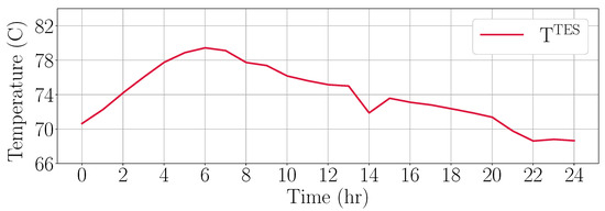
Figure 11.
The TES temperature across 24 h with standard MPC and no plant–model mismatch.
4.2. Standard vs. Multistage MPC
Next, we compare the results of the standard and multistage MPC applied to the TES system. We focus on the operating constraints in the system for this demonstration. The supply of heat on the supplier side is assumed to come from a batch cooling process, which requires that the return temperature does not exceed 85 °C. As such, any temperatures above the mandated limit may lead to inferior product quality in the batches. Similarly, the district heating network on the consumer side needs the return temperature to be above 60 °C. Therefore, any constraint violation on these return temperatures carries an economic penalty for the respective supplier or consumer. The initial values of the process temperatures, and , are 91.28 °C and 50 °C respectively. The initial temperature in the tank is 70.63 °C. These values are obtained from the steady-state optimization of the system for mean values of heat supply and demand.
To investigate the robustness of the methods, the actual heat supply and demand profiles of 6 January 2018 are considered. The expected values in both the MPC formulations come from the 2017 data, as do the scenarios of multistage MPC method. The difference in the 2017 and 2018 data creates the plant–model mismatch. Figure 12 shows the supplier return, consumer return, and the tank temperature profiles obtained by the application of the two control strategies, given the constraints on the return temperatures. It can be seen that the temperature profiles are higher with multistage MPC in general. The multistage MPC keeps the tank heated up and discharges it less than the standard MPC, even though there is a higher demand. This conservativeness is because the multistage MPC respects the constraint on consumer-side return temperature to keep it above 60 °C. In contrast, the standard MPC violates this operating constraint during 8 out of the 24 h of operation, since it prioritizes the economic objective of demand satisfaction at the cost of constraint violation. The multistage MPC, having accounted for such a scenario in its scenario-tree formulation, anticipates that recourse action is possible in the future time steps. As a consequence, is always above its limit in order to satisfy consumer demand, and does not violate it.
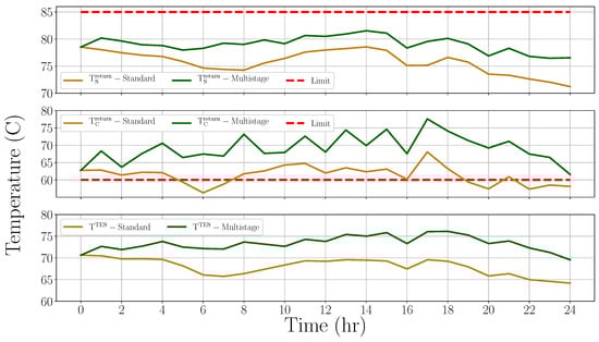
Figure 12.
The supplier return, consumer return, and tank temperature profiles in the standard and multistage MPC formulations, for 6 January 2018.
Multistage MPC, however, has a higher cost of peak heating than standard MPC, as shown in Figure 13. While standard MPC suggests a total peak heating of 42.15 MWh, multistage MPC results in 88.73 MWh of peak heating across the day. This can be thought of as the “cost of robustness” required by multistage MPC. Since can only drop so much, the remaining heat demand has to be satisfied through additional peak heating. The supplier also has to dump a lot of heat compared to standard MPC, since the temperature of the return stream has to be brought down below 85 °C. Another factor is the temperature difference between the supplier and the TES, which becomes too small to transfer heat. Figure 13 also shows the differences in the actual and expected heat supply and demand profiles. The standard MPC is oblivious to these differences in the heat supply and demand, and proposes control solutions that require lesser peak heating. The plant–model mismatch that arises from this uncertainty, however, causes the states to violate their operating constraints. Although the standard MPC suggests lower peak heating requirements compared to multistage MPC, this is counterproductive because it is not robust and ends up violating the operating constraint for a significant operating period. The economic penalty of such suboptimal operation may be significantly higher than any savings achieved via lower peak heating.
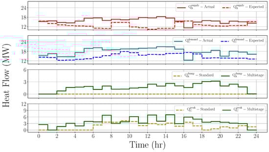
Figure 13.
The heat supply and demand profiles; and the corresponding heat dumping and peak heating profiles obtained from standard and multistage MPC formulations for 6 January 2018.
We repeated the simulations for all days of January 2018 using the corresponding heat supply and demand profiles, and found that multistage MPC is consistently successful in keeping the system within the specified limits, whereas the standard MPC frequently results in constraint violations. This can be seen in Figure 14, which shows the supplier and consumer return temperature profiles for all the days in January 2018. These simulations show the applicability of the method even when the heat supply at the start of the horizon is lower than the heat demand, as was the case for multiple days in January 2018.
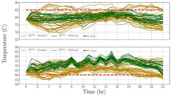
Figure 14.
The supplier and consumer return temperature profiles for the whole month of January 2018; standard MPC leads to frequent constraint violations, multistage MPC keeps the temperatures within bounds.
The robustness offered by multistage MPC comes with a higher peak heating cost. The average daily use of peak heating across all days in January with standard MPC is found to be 17.27 MWh, whereas for multistage MPC it is 73.11 MWh. We also noted the frequency of constraint violations in both cases. The supplier and consumer-side return temperature constraints are violated during a daily average of 3.2 h and 3.6 h respectively for standard MPC. The corresponding values for multistage MPC are 0.06 h and 0.03 h respectively. This shows that the cluster operator is better off employing the multistage MPC strategy even though it has higher peak heating cost. This is because the long periods of unprofitable operation in standard MPC may not be acceptable to the stakeholders, resulting in higher overall costs. Multistage MPC thus helps to keep the overall costs down, while also making the system robust against uncertainties in heat supply and demand.
5. Conclusions
In this paper, the application of multistage MPC strategy was investigated for an industrial cluster system with a hot water TES unit. The case study presented a model with one supplier and one consumer of surplus heat, whereby the heat exchange happens through a TES tank. The model was derived using energy balances over the various system components. The surplus heat exchange in the cluster with a TES was found to be much more cost-effective compared to a corresponding system without TES. We further looked at the challenge of effectively handling the uncertainty in heat supply and demand for this system, with the proposed multistage MPC scheme. A scenario-tree formulation for the uncertain supply and demand was implemented, and the robustness of this strategy was demonstrated by comparing it to a standard MPC formulation where uncertainty is not taken into account. The scenario selection in the multistage MPC is done via the data-driven PCA algorithm, which results in a computationally efficient but robust formulation. We use additional data analysis to detect outliers in the data and to predict trends in the heat profiles.
The results demonstrated that although the multistage MPC is more conservative than the equivalent standard MPC formulation in terms of peak heating requirements (the “cost of robustness”), it is much better at keeping the system within specified bounds on the system states. We considered operating constraints on the return temperatures on the supplier and consumer plants, and found that a standard MPC strategy leads to frequent, non-trivial, constraint violations. The multistage MPC, on the other hand, was able to steer the system while respecting these operating constraints and was also not overly conservative. We argue that large economic penalties for constraint violations justify the use of the multistage MPC strategy over standard MPC, as it is more effective in handling the uncertain heat supply and demand. In a nutshell, we demonstrated that implementing the proposed robust control strategy can result in an energy-efficient utilization of the TES unit for surplus heat exchange, not only providing cost-savings to the industrial cluster as a whole, but also benefiting its individual stakeholders.
Author Contributions
Conceptualization, M.T. and J.J.; Methodology, M.T. and J.J.; Software, M.T. and Z.M.; Formal analysis, M.T., Z.M. and J.J.; Investigation, M.T., Z.M. and J.J.; Resources, M.T., Z.M. and J.J.; Data curation, M.T. and Z.M.; Writing—original draft preparation, M.T.; Writing—review and editing, M.T., Z.M. and J.J.; Supervision, J.J.; Project administration, J.J. All authors have read and agreed to the published version of the manuscript.
Funding
This publication has been funded by HighEFF - Centre for an Energy Efficient and Competitive Industry for the Future, an 8-year Research Centre under the FME-scheme (Centre for Environment-friendly Energy Research, 257632). The authors gratefully acknowledge the financial support from the Research Council of Norway and user partners of HighEFF.
Acknowledgments
The authors thank Mo Fjernvarme AS for providing industrial data on heat supply and demand. The authors also appreciate valuable inputs from Brage Rugstad Knudsen, SINTEF Energy Research.
Conflicts of Interest
The authors declare no conflict of interest.
Abbreviations
| Q | Heat flow rate (kW) |
| T | Temperature (°C) |
| q | Volumetric flow rate (ms) |
| heat transfer conductance (kW/°C) | |
| V | Volume (m) |
| Density (kg/m) | |
| Specific heat capacity (kJ/kg°C) | |
| PID | Proportional-Integral-Derivative |
| TES | Thermal Energy Storage |
| MPC | Model Predictive Control |
| ODE | Ordinary Differential Equations |
| NLP | Nonlinear Program |
| PCA | Principal Component Analysis |
| Probability Distribution Function |
Appendix A. Detailed Heat Exchanger Model Equations
The vector-valued functions and are expanded upon in this appendix. A full schematic of the process used for model derivation is shown in Figure A1.

Figure A1.
Detailed model illustration for the heat exchangers in the TES. The red and blue lines represent the hot and cold streams respectively.
Figure A1.
Detailed model illustration for the heat exchangers in the TES. The red and blue lines represent the hot and cold streams respectively.

We apply enthalpy balances over the components shown in Figure A1, namely the process and return pipe elements, as well as the hot and cold sides of the heat exchanger. Note that we consider countercurrent flow in the heat exchangers. The enthalpy balance over the process pipe element yields:
Similarly, the enthalpy balance over the return pipe element gives:
The balances over the hot and cold sides of the supplier-side heat exchanger lead to the following equations:
The Equations (A1)–(A4) together form the vector-valued function . The enthalpy balances for the consumer side are analogous to . The enthalpy balance for the process pipe element leads to:
Similarly, the balance over the consumer-side return pipe element yields:
Finally, the enthalpy balances over the hot and cold sides on the consumer-side heat exchanger result in the following equations:
It may be noted from Figure A1 that the volumetric flow rates of water going in and out of the TES are equal. The volume of the water inside the TES is thus always constant.
Appendix B. Dynamic Optimization Problem for the TES System
The complete formulation of the dynamic optimization problem for the industrial park system with one supplier, one consumer and a TES tank is as follows:
Appendix C. Data Preprocessing for Outlier Detection
Here is a more detailed explanation of how the data was treated to detect outliers. The data set was limited to winter months of January–March and December when thermal energy storage is applicable. This resulting supply and demand data sets each had 121 sample days with 24 hourly measurements in each day. PCA was performed separately on the supply and demand data matrices each of dimensions , resulting into two models. Since we aim at finding a linear correlation between supply and demand, then we detect outlier samples appearing in either of the two PCA models. The supply data PCA model covered a total variance of about 89.90% using 7 principal components. On the other hand, demand data PCA model captured more variation with fewer components and achieved a total explained variance of 95.58% using 6 principal components.

Figure A2.
Influence plots for demand and supply data in the winter months (January–March and December). The confidence interval was set to 95% and the limits are shown as red-dashed lines. Samples with either high Hotelling’s or F-Residuals (F-distributed) are considered outliers. The outliers are labelled with their corresponding date.

Determination of an outlier was done by calculation of sample residuals and leverage in each PCA model. Leverage is the distance of the sample point from the origin of the PCA model measured along the new model subspace. A sample with high leverage implies over-influence on the PCA model, making it not a general representation of the system. Samples with significantly higher residuals and leverage compared to the others are considered outliers. This is a statistical anomaly detection which can be applied to processes as explained in [38,39]. The sample residuals are estimated to be F-distributed and the X-residuals were converted to F-residuals. A multivariate t-test on the PCA scores (not the original variables) is called the Hotelling’s statistic [40]. The Hotelling’s statistic is directly related to the leverage of the sample on the PCA model. It is also approximated as being F-distributed. The critical limits for Hotelling’s and F-residuals were estimated such that the confidence interval was 95%. A plot of F-residual against Hotelling’s shown in Figure A2, called the influence plot, represents the outlier analysis for supply and demand data sets.
The samples that were above the critical limits (red-dashed lines) in either F-residual and Hotelling’s statistic were considered outliers and were discarded from further analysis. In the Figure A2, the outliers corresponding to the months of January and December are numbered with their corresponding date.
References
- International Energy Agency. 2019. Available online: https://www.iea.org/topics/energyefficiency/industry/ (accessed on 6 April 2019).
- Brückner, S.; Miró, L.; Cabeza, L.F.; Pehnt, M.; Lävemann, E. Methods to estimate the industrial waste heat potential of regions—A categorization and literature review. Renew. Sustain. Energy Rev. 2014, 38, 164–171. [Google Scholar] [CrossRef]
- Chertow, M.R. “Uncovering” Industrial Symbiosis. J. Ind. Ecol. 2007, 11, 11–30. [Google Scholar] [CrossRef]
- Fang, H.; Xia, J.; Jiang, Y. Key issues and solutions in a district heating system using low-grade industrial waste heat. Energy 2015, 86, 589–602. [Google Scholar] [CrossRef]
- Rodera, H.; Bagajewicz, M.J. Targeting procedures for energy savings by heat integration across plants. AIChE J. 1999, 45, 1721–1742. [Google Scholar] [CrossRef]
- Boix, M.; Montastruc, L.; Azzaro-Pantel, C.; Domenech, S. Optimization methods applied to the design of eco-industrial parks: A literature review. J. Clean. Prod. 2015, 87, 303–317. [Google Scholar] [CrossRef]
- Zhang, B.J.; Zhang, Z.L.; Liu, K.; Chen, Q.L. Network Modeling and Design for Low Grade Heat Recovery, Refrigeration, and Utilization in Industrial Parks. Ind. Eng. Chem. Res. 2016, 55, 9725–9737. [Google Scholar] [CrossRef]
- Kuznetsova, E.; Zio, E.; Farel, R. A methodological framework for Eco-Industrial Park design and optimization. J. Clean. Prod. 2016, 126, 308–324. [Google Scholar] [CrossRef]
- Hassiba, R.J.; Linke, P. On the simultaneous integration of heat and carbon dioxide in industrial parks. Appl. Therm. Eng. 2017, 127, 81–94. [Google Scholar] [CrossRef]
- Anastasovski, A.; Rašković, P.; Guzović, Z. Design and analysis of heat recovery system in bioprocess plant. Energy Convers. Manag. 2015, 104, 32–43. [Google Scholar] [CrossRef]
- Brückner, S.; Liu, S.; Miró, L.; Radspieler, M.; Cabeza, L.F.; Lävemann, E. Industrial waste heat recovery technologies: An economic analysis of heat transformation technologies. Appl. Energy 2015, 151, 157–167. [Google Scholar] [CrossRef]
- De Oliveira, V.; Jäschke, J.; Skogestad, S. Optimal operation of energy storage in buildings: Use of the hot water system. J. Energy Storage 2016, 5, 102–112. [Google Scholar] [CrossRef]
- Ma, Y.; Kelman, A.; Daly, A.; Borrelli, F. Predictive Control for Energy Efficient Buildings with Thermal Storage: Modeling, Stimulation, and Experiments. IEEE Control. Syst. Mag. 2012, 32, 44–64. [Google Scholar] [CrossRef]
- Tang, R.; Wang, S. Model predictive control for thermal energy storage and thermal comfort optimization of building demand response in smart grids. Appl. Energy 2019, 242, 873–882. [Google Scholar] [CrossRef]
- Labidi, M.; Eynard, J.; Faugeroux, O.; Grieu, S. Predictive Control and Optimal Design of Thermal Storage Systems for Multi-energy District Boilers. IFAC Proc. Vol. 2014, 47, 10305–10310. [Google Scholar] [CrossRef]
- Powell, K.M.; Edgar, T.F. Control of a large scale solar thermal energy storage system. In Proceedings of the 2011 American Control Conference, San Francisco, CA, USA, 29 June–1 July 2011; pp. 1530–1535. [Google Scholar] [CrossRef]
- Knudsen, B.R.; Kauko, H.; Andresen, T. An Optimal-Control Scheme for Coordinated Surplus-Heat Exchange in Industry Clusters. Energies 2019, 12, 1877. [Google Scholar] [CrossRef]
- Miró, L.; Gasia, J.; Cabeza, L.F. Thermal energy storage (TES) for industrial waste heat (IWH) recovery: A review. Appl. Energy 2016, 179, 284–301. [Google Scholar] [CrossRef]
- Sarbu, I.; Sebarchievici, C. A Comprehensive Review of Thermal Energy Storage. Sustainability 2018, 10, 191. [Google Scholar] [CrossRef]
- Cole, W.; Powell, K.; Edgar, T. Optimization and advanced control of thermal energy storage systems. Rev. Chem. Eng. 2012, 28, 81–99. [Google Scholar] [CrossRef]
- Huang, F.; Zheng, J.; Baleynaud, J.; Lu, J. Heat recovery potentials and technologies in industrial zones. J. Energy Inst. 2017, 90, 951–961. [Google Scholar] [CrossRef]
- Lucia, S.; Finkler, T.; Engell, S. Multi-stage nonlinear model predictive control applied to a semi-batch polymerization reactor under uncertainty. J. Process. Control. 2013, 23, 1306–1319. [Google Scholar] [CrossRef]
- Campo, P.J.; Morari, M. Robust Model Predictive Control. In Proceedings of the 1987 American Control Conference, Minneapolis, MN, USA, 10–12 June 1987; pp. 1021–1026. [Google Scholar]
- de Nicolao, G.; Magni, L.; Scattolini, R. On the robustness of receding-horizon control with terminal constraints. IEEE Trans. Autom. Control. 1996, 41, 451–453. [Google Scholar] [CrossRef]
- Candès, E.J.; Wakin, M.B.; Boyd, S.P. Enhancing Sparsity by Reweighted l1 Minimization. J. Fourier Anal. Appl. 2008, 14, 877–905. [Google Scholar] [CrossRef]
- Biegler, L.T. Nonlinear Programming: Concepts, Algorithms, and Applications to Chemical Processes; SIAM: Philadelphia, PA, USA, 2010; Volume 10. [Google Scholar]
- Rawlings, J.; Mayne, D. Model Predictive Control: Theory and Design; Nob Hill Pub.: Portland, OR, USA, 2009. [Google Scholar]
- Grüne, L.; Stieler, M. Asymptotic stability and transient optimality of economic MPC without terminal conditions. J. Process. Control. 2014, 24, 1187–1196. [Google Scholar] [CrossRef]
- Krishnamoorthy, D.; Foss, B.; Skogestad, S. A Distributed Algorithm for Scenario-based Model Predictive Control using Primal Decomposition. IFAC-PapersOnLine 2018, 51, 351–356. [Google Scholar] [CrossRef]
- Lucia, S.; Engell, S. Robust nonlinear model predictive control of a batch bioreactor using multi-stage stochastic programming. In Proceedings of the IEEE 2013 European Control Conference (ECC), Zurich, Switzerland, 17–19 July 2013; pp. 4124–4129. [Google Scholar] [CrossRef]
- Krishnamoorthy, D.; Thombre, M.; Skogestad, S.; Jäschke, J. Data-driven Scenario Selection for Multistage Robust Model Predictive Control. IFAC-PapersOnLine 2018, 51, 462–468. [Google Scholar] [CrossRef]
- Thombre, M.; Krishnamoorthy, D.; Jäschke, J. Data-driven Online Adaptation of the Scenario-tree in Multistage Model Predictive Control. IFAC-PapersOnLine 2019, 52, 461–467. [Google Scholar] [CrossRef]
- Jolliffe, I.T.; Cadima, J. Principal component analysis: A review and recent developments. Philos. Trans. Ser. Math. Phys. Eng. Sci. 2016, 374, 20150202. [Google Scholar] [CrossRef]
- Dunning, I.; Huchette, J.; Lubin, M. JuMP: A Modeling Language for Mathematical Optimization. SIAM Rev. 2017, 59, 295–320. [Google Scholar] [CrossRef]
- Bezanson, J.; Edelman, A.; Karpinski, S.; Shah, V. Julia: A Fresh Approach to Numerical Computing. SIAM Rev. 2017, 59, 65–98. [Google Scholar] [CrossRef]
- Wächter, A.; Biegler, L.T. On the implementation of an interior-point filter line-search algorithm for large-scale nonlinear programming. Math. Program. 2006, 106, 25–57. [Google Scholar] [CrossRef]
- STFC Rutherford Appleton Laboratory. HSL. A Collection of Fortran Codes for Large Scale Scientific Computation. 2019. Available online: http://www.hsl.rl.ac.uk/ (accessed on 6 April 2019).
- Eriksson, L.; Byrne, T.; Johansson, E.; Trygg, J.; Vikström, C. Multi-And Megavariate Data Analysis Basic Principles and Applications; MKS Umetrics AB: Malmö, Sweden, 2013; Volume 1. [Google Scholar]
- Harrou, F.; Kadri, F.; Chaabane, S.; Tahon, C.; Sun, Y. Improved principal component analysis for anomaly detection: Application to an emergency department. Comput. Ind. Eng. 2015, 88, 63–77. [Google Scholar] [CrossRef]
- Hotelling, H. Analysis of a complex of statistical variables into principal components. J. Educ. Psychol. 1933, 24, 417. [Google Scholar] [CrossRef]


© 2020 by the authors. Licensee MDPI, Basel, Switzerland. This article is an open access article distributed under the terms and conditions of the Creative Commons Attribution (CC BY) license (http://creativecommons.org/licenses/by/4.0/).