Article

Extreme Learning Machine Based on Firefly Adaptive Flower Pollination Algorithm Optimization

1
School of Science, Xi’an Polytechnic University, Xi’an 710048, China
2
School of Mathematics and Information Science, Guangzhou University, Guangzhou 510006, China
*
Author to whom correspondence should be addressed.
Processes 2020, 8(12), 1583; https://doi.org/10.3390/pr8121583
Submission received: 30 September 2020 / Revised: 26 October 2020 / Accepted: 2 November 2020 / Published: 1 December 2020
(This article belongs to the Section Process Control and Monitoring)

Abstract

:
Extreme learning machine (ELM) has aroused a lot of concern and discussion for its fast training speed and good generalization performance, and it has been used diffusely in both regression and classification problems. However, on account of the randomness of input parameters, it requires more hidden nodes to obtain the desired accuracy. In this paper, we come up with a firefly-based adaptive flower pollination algorithm (FA-FPA) to optimize the input weights and thresholds of the ELM algorithm. Nonlinear function fitting, iris classification and personal credit rating experiments show that the ELM with FA-FPA (FA-FPA-ELM) can obtain significantly better generalization performance (such as root mean square error, classification accuracy) than traditional ELM, ELM with firefly algorithm (FA-ELM), ELM with flower pollination algorithm (FPA-ELM), ELM with genetic algorithm (GA-ELM) and ELM with particle swarm optimization (PSO-ELM) algorithms.

1. Introduction

For the past few years, various artificial intelligence algorithms have attracted more and more attention from scientific research and industrial applications. Machine learning, also known as statistical learning theory, is an important branch of artificial intelligence. It obtains data laws through data analysis and applies these laws to predict or determine other unknown data. Machine learning has been diffusely used in data mining [1], natural language processing [2], speech recognition [3] and search engines [4]. Neural network is a crucial algorithm for machine learning. It changes the internal structure of the system by sensing changes in external information. Feedforward neural networks [5] are one of the most widely used neural networks. It generally includes an input layer, a hidden layer and an output layer, where the hidden layer can be multi-layered. Neurons in the same layer are not connected, and adjacent layers have multiple connection methods. The back layer only receives information from the front layer. Typical feedforward neural networks include perceptron models [6], BP neural networks [7], self-coding neural networks [8], radial basis networks [9,10] and convolutional neural networks [11].
Lately, ELM was put forward by Huang et al. [12,13,14,15]. This is a novel algorithm for single hidden layer feedforward network [16,17,18,19]. It randomly generates input weights and thresholds, and can directly calculate output weights. The learning speed of ELM algorithm is much faster than the feedforward network learning algorithm based on the gradient descent, and it has good generalization performance on complex application problems [20,21]. However, because the input parameters are randomly generated, ELM requires a lot of hidden neurons, otherwise it will fall into local minima and overfitting problems [22]. The accuracy and availability of the ELM algorithm largely depend on the parameters of the internal model. In order to select the appropriate model parameters, many researchers use bio-inspired optimization algorithms to optimize the input weights and thresholds. In [23], Zhu et al. proposed a hybrid learning algorithm that uses the differential evolutionary algorithm to select the input weights, and then uses Moore–Penrose (MP) generalized inverse to determine the output weights. Experimental consequences show that the method has good generalization performance in a more compact network. Ling and Han [24] proposed an input weights and hidden thresholds selection algorithm based on particle swarm optimization for ELM (PSO-ELM). Compared with the original ELM and other evolved ELMs, PSO-ELM has better generalization performance in function approximation and benchmark classification experiments. In [25], Alexandre and Cuadra proposed a novel feature selection method that combines a special genetic algorithm and ELM (GA-ELM feature selection algorithm). After a lot of comparison experiments, it is found that this method has a good classification effect. Wu et al. [26] used four biologically-inspired algorithms to optimize ELM to predict China’s daily evapotranspiration (ETo). These are GA-ELM, ELM with ant colony optimization (ACO-ELM), ELM with cuckoo search algorithm (CSA-ELM) and ELM with flower pollination algorithm (FPA-ELM). The research results show that CSA-ELM and FPA-ELM have better prediction performance.
Flower pollination algorithm (FPA) [27,28,29] and firefly algorithm (FA) [30,31,32,33,34] are two new heuristic swarm intelligence optimization algorithms proposed by Yang. FPA has the advantages of few parameters, easy adjustment and simple implementation. When solving multi-objective optimization problems, the performance of FPA is better than GA and PSO [35,36,37,38,39,40,41,42]. The principle of the FA-FPA is to use the FA algorithm to get a better initial position before the FPA algorithm. As a resul that the position obtained after FA iteration helps to accelerate the convergence rate of FPA and find the global optimal solution. In this paper, our strategy is to combine FA-FPA with original ELM, proposing an algorithm for optimizing ELM based on FA-FPA. The basic idea of FA-FPA-ELM algorithm is to first use FA-FPA to find the best input weights and thresholds of ELM, and then use MP generalized inverse to determine the output weights. The main contributions are as follows.
  • It is shown how to use FA-FPA to train ELM. This method can optimize the input weights and thresholds of ELM algorithm, so as to achieve the goal of finding the optimal parameter combination.
  • Finding the optimal parameters of the ELM algorithm through FA-FPA can effectively solve the problem of local minima and overfitting, and enhance the generalization capability of the network.
  • Nonlinear function fitting, iris classification and personal credit rating problems show that the FA-FPA-ELM algorithm can obtain better generalization performance than traditional ELM, FA-ELM, FPA-ELM, GA-ELM and PSO-ELM algorithms.
The rest of the paper is arranged as follows: Section 2 describes the network structure of traditional ELM algorithm. Section 3 describes the theory and implementation steps of the FA-FPA. Section 4 describes how to optimize ELM network parameters based on FA-FPA. The capability of the FA-FPA-ELM algorithm is compared with ELM, FA-ELM, FPA-ELM, GA-ELM and PSO-ELM algorithms by nonlinear function fitting, iris classification and personal credit rating problems in Section 5. In the end, the conclusion is given in Section 6.

2. Extreme Learning Machine (ELM)

ELM mechanism is described as follows. The number of neurons in the input layer, hidden layer and output layer are n, L and m, respectively, and the network structure diagram is shown in Figure 1. ELM algorithm randomly generates input weights and thresholds, only by setting the quantity of hidden nodes, and can acquire the unique ideal solution. Suppose there are Q different training samples, where X and Y are input data and output data, respectively
X = x 11 x 12 x 1 Q x 21 x 22 x 2 Q x n 1 x n 2 x n Q n × Q
Y = y 11 y 12 y 1 Q y 21 y 22 y 2 Q y m 1 y m 2 y m Q m × Q
the actual output T of the network is as follows:
T = t 11 t 12 t 1 Q t 21 t 22 t 2 Q t m 1 t m 2 t m Q m × Q
The standard ELM with L hidden nodes can be denoted as
i = 1 L β i φ i ( x j ) = i = 1 L β i φ ( w i · x j + b i ) = t j
where t j = [ t 1 j , t 2 j , , t m j ] T , φ ( x ) represents activation function, the specific expression of t j is as follows:
t j = i = 1 L β i 1 φ ( w i · x j + b i ) i = 1 L β i 2 φ ( w i · x j + b i ) i = 1 L β i m φ ( w i · x j + b i ) m × 1
where j = 1 , 2 , , Q , x j = [ x 1 j , x 2 j , , x n j ] T , w i = [ w i 1 , w i 2 , , w i n ] is the weight vector concatenating the i-th hidden node and input nodes, β i = [ β i 1 , β i 2 , , β i m ] T is the weight vector concatenating the i-th hidden node and output nodes and b i is the threshold of the i-th hidden node. w i · x j denotes the inner product of w i and x j .
The above (5) can be signified as H β = T T , where H is the output matrix of the hidden layer. Its specific form is
H ( w 1 , , w L , b 1 , , b L , x 1 , , x Q ) = φ ( w 1 · x 1 + b 1 ) φ ( w L · x 1 + b L ) φ ( w 1 · x 2 + b 1 ) φ ( w L · x 2 + b L ) φ ( w 1 · x Q + b 1 ) φ ( w L · x Q + b L ) Q × L
the least squares solutions of formula H β = T T can be represented as:
β ^ = H T T
here, H is the MP generalized inverse of hidden layer output matrix H.

3. Firefly-Based Adaptive Flower Pollination Algorithm (FA-FPA)

3.1. Adaptive Flower Pollination Algorithm (FPA)

There are two ways to achieve pollination: self-pollination and cross-pollination. Self-pollination usually occurs when there is no reliable pollinator and is fertilized from the pollen of the same plant. Cross-pollination means that pollination can be conducted from pollen of different plants. Cross-pollination usually involves bees, bats and birds, and these pollinators can fly a long distance. The behavior of bees and birds will follow the l e ´ v y distribution [43]. For the convenience of research, it is premised that each plant has only one flower and one pollen gamete. Each pollen gamete maintains a one-to-one relationship with a solution, and the corresponding pollination process follows the following rules.
  • Cross-pollination can be deemed a global pollination process, while pollinators carrying pollen move in a way that follows l e ´ v y flights.
  • Self-pollination can be seen as a process of local pollination.
  • The constancy of the flower is the probability of reproduction, which is proportional to the similarity of the two flowers involved.
  • The switch probability p [ 0 , 1 ] can adjust local pollination and global pollination. Owing to the influence of distance and other factors, the whole pollination process is more inclined to local pollination.
In the initial stage of FPA, randomly generate a population P ( t ) = { X t i } of N individuals, X t i = [ x i , 1 t , x i , 2 t , , x i , j t , , x i , D t ] ( j = 1 , 2 , , D ; i = 1 , 2 , , N ) , where N is the size of the population, D is the dimension of the optimization problem and t is the current number of iterations. Self-pollination is the process of local pollination, the process is as follows:
X i t + 1 = X i t + ε ( X j t X i t )
where X j t , X i t represent pollen of different flowers of the same plant, i , j are random integers on [1, N]. The variation factor ε is a random number obeying uniform distribution on [0, 1].
Cross-pollination is a global pollination process by pollinators through l e ´ v y flight, the process is as follows:
X i t + 1 = X i t + γ L ( X i t g * )
here, X i t represents the position of pollen i at the t-th iteration, g * represents the optimal solution of the current group, γ represents the scaling factor of the control step, L represents the intensity of pollination, which substantially is a step size and it follows the l e ´ v y distribution. In the basic FPA, the conversion probability p is a constant, which may cause the problem that the algorithm is not easy to converge and fall into the local optimal solution. Therefore, the following adaptive adjustments are made to p:
p = 0.8 + 0.2 σ
where σ is a random number between [−1, 1]. In reference [44], when p is 0.8, the algorithm has the best performance, so p is set to float around 0.8 to prevent the value of p from being too large or too small. The improved algorithm can adaptively adjust the execution probability of global search and local search, avoiding FPA from falling into local optimum, and at the same time improving the convergence speed of the algorithm.

3.2. Firefly Algorithm (FA)

In nature, fireflies communicate with other fireflies through their own light-emitting characteristics. The FA regards the problem of solving the optimal value as the problem of finding the brightest fireflies, and simulates the entire optimization process as the process of mutual attraction and iterative update of fireflies. To simplify the algorithm, make the following assumptions:
  • Regardless of the sex of the fireflies.
  • The attraction between fireflies is only pertinent to the brightness and distance of fireflies.
  • The brightness of fireflies is determined by the fitness function.
The brighter the firefly is, the better its position is. Fireflies that glow weaker will move to brighter ones. The brightest firefly represents the optimal solution of the function. If the brightness is the same, the firefly will move randomly. If the distance between individual j and individual i is r i j , then the brightness at individual j is
I i j = I 0 × e λ r i j
among them, λ is the light intensity absorption coefficient, the general value is 1.0, I 0 is the maximum fluorescent brightness of fireflies, r i j denotes the Euclidean distance between firefly i and firefly j and its expression is as follows:
r i j = x j x i = k = 1 d ( x j k x i k ) 2
the attraction between individual j and individual i can be expressed as
β i j = β 0 e λ r i j 2
where β 0 is the maximum attraction of fireflies. If firefly j is attracted and moved by another brighter firefly i, its position update formula is:
X j t + 1 = X j t + β 0 e λ r i j 2 ( X i t X j t ) + α μ j
here, α is the step factor, μ j is a random vector and the random numbers in the vector follow Gaussian distribution or uniform distribution. The position of fireflies is constantly updated through brightness and attraction. Eventually, most fireflies will gather around fireflies with higher fitness values, and finally achieve the purpose of optimization.

3.3. Firefly-Based Adaptive Flower Pollination Algorithm (FA-FPA)

Since FA adopts a global random search strategy with multiple positions in parallel, the position obtained after iteration helps accelerate the convergence of adaptive FPA and find the global optimal solution. Therefore, FA can be used to obtain a better initial position, and then use FPA optimization. The specific algorithm process is shown in Table 1.

4. Firefly Adaptive Flower Pollination Extreme Learning Machine Algorithm (FA-FPA-ELM)

For effectively solving this question caused by the randomness of the input parameters of the ELM algorithm, this paper uses the FA-FPA with strong optimization ability to optimize the ELM input weights and thresholds, so as to propose an adaptive FA-FPA-ELM algorithm. We first use FA-FPA to obtain the optimal weights and thresholds combination, and use it directly as the input weights and thresholds for ELM training. For decreasing the influence on the performance of the algorithm due to the large difference in variables, we use Equation (15) to normalize the data:
X = X X m i n X m a x X m i n
here, X m a x , X m i n respectively denote the maximum and minimum values in the training samples.
Next, we individually encode the ELM input parameters, the input weights and thresholds are expressed as individual pollen in the form of real coding. According to Section 2, the number of neurons in the input layer and hidden layer are n and L, respectively; therefore, the string length of individual pollen is
ρ = n × L + L
assume that the weight matrix ω connecting the input layer and the hidden layer is
ω = ω 11 ω 12 ω 1 n ω 21 ω 22 ω 2 n ω L 1 ω L 2 ω L n L × n
the threshold vector b of the hidden layer is
b = [ b 1 , b 2 , , b L ] T
then the coding form of the individual pollen is
X = [ ω 11 , , ω 1 n , ω 21 , , ω 2 n , , ω L n , b 1 , , b L ]
The fitness function used in FA-FPA is the root mean square error (RMSE). The RMSE and mean absolute error (MAE) between the actual output and the expected output of the network are used as the evaluation standard of the network. The following formula are used to calculate RMSE and MAE
R M S E = i = 1 n [ f ( x i ) y i ] 2 n , M A E = i = 1 n f ( x i ) y i ) n
where f ( x i ) denotes the predicted datas, y i denotes the actual datas. Therefore, the purpose of using FA-FPA to optimize ELM input parameters is to find pollen particles that can make the RMSE of the ELM algorithm smaller. Table 2 details the implementation steps of the FA-FPA-ELM algorithm.

5. Numerical Experiments and Comparison

To verify the effectiveness of the introduced FA-FPA-ELM algorithm, we have done some experiments which are nonlinear function fitting, iris classification and personal credit rating problems. This section compares the approximation and classification performance of FA-FPA-ELM with traditional ELM, FA-ELM, FPA-ELM, GA-ELM and PSO-ELM algorithms.

5.1. Nonlinear Function Fitting Problem

The nonlinear function defined by
f ( x ) = 1.1 ( 1 x + 2 x 2 ) e x 2 / 2
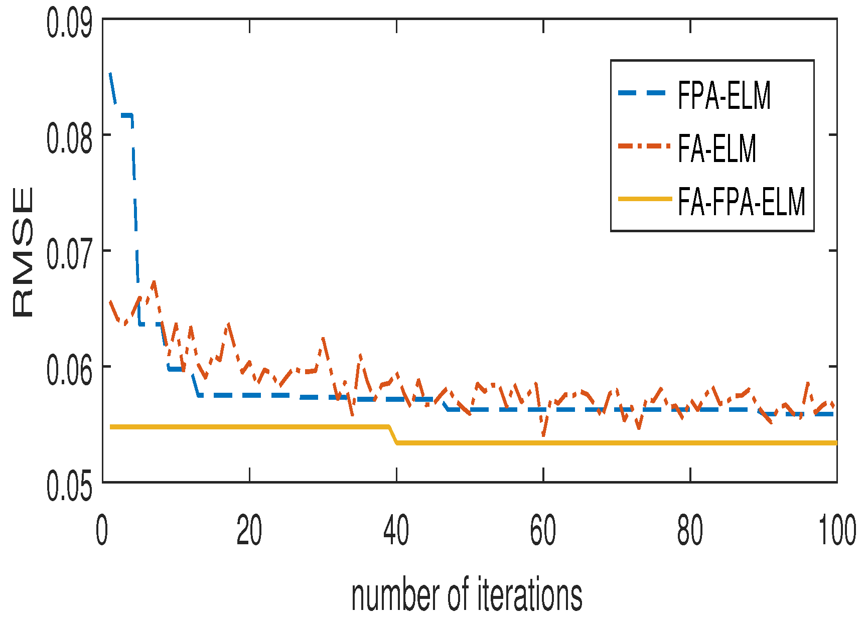
a training set ( x i , f ( x i ) ) with 400 data, where x i follows the uniform distribution of [−10, 10]. In order to prevent overfitting and improve the generalization performance of the algorithm, add noise ζ i with uniform distribution of [−0.1, 0.1] to the training samples, then the final training sample is ( x i , f ( x i ) + ζ i ) . At the same time, we select 100 test samples ( x i , f ( x i ) ) , where x i is the equal interval sampling of [−10, 10]. For FA, a step factor of α = 0.25 , a maximum attraction of β 0 = 0.2 and a absorption coefficient of light intensity λ = 1 are used. For FPA, the initial value of the conversion probability p = 0.8 , and the same population size N = 10 have been used for two algorithms. The fitness function is the RMSE for the training sample. The activation function is a radial basis function. It can be seen from Figure 2 that the FA-ELM algorithm will fall into the local optimum when optimizing the ELM parameters. The improved FA-FPA-ELM algorithm can jump out of the local optimum and accelerate the convergence speed of the FPA-ELM. For the sake of testing the effect of the quantity of iterations on the performance of the FA-FPA-ELM algorithm, we set the hidden layer neurons to 5, and the number of iterations was taken as i = 5, 10, 20, 50, 100 and 500. Perform 30 experiments respectively, and then take the average of training time, test time, RMSE and MAE. The experimental results are demonstrated in Table 3. Next, we test the impact of the number of hidden nodes on the ELM and FA-FPA-ELM algorithms. The maximum number of iterations is set to 100. When the number of hidden layer nodes gradually increases, the training time and RMSE of the two continue to change. The experimental results are demonstrated in Table 4.
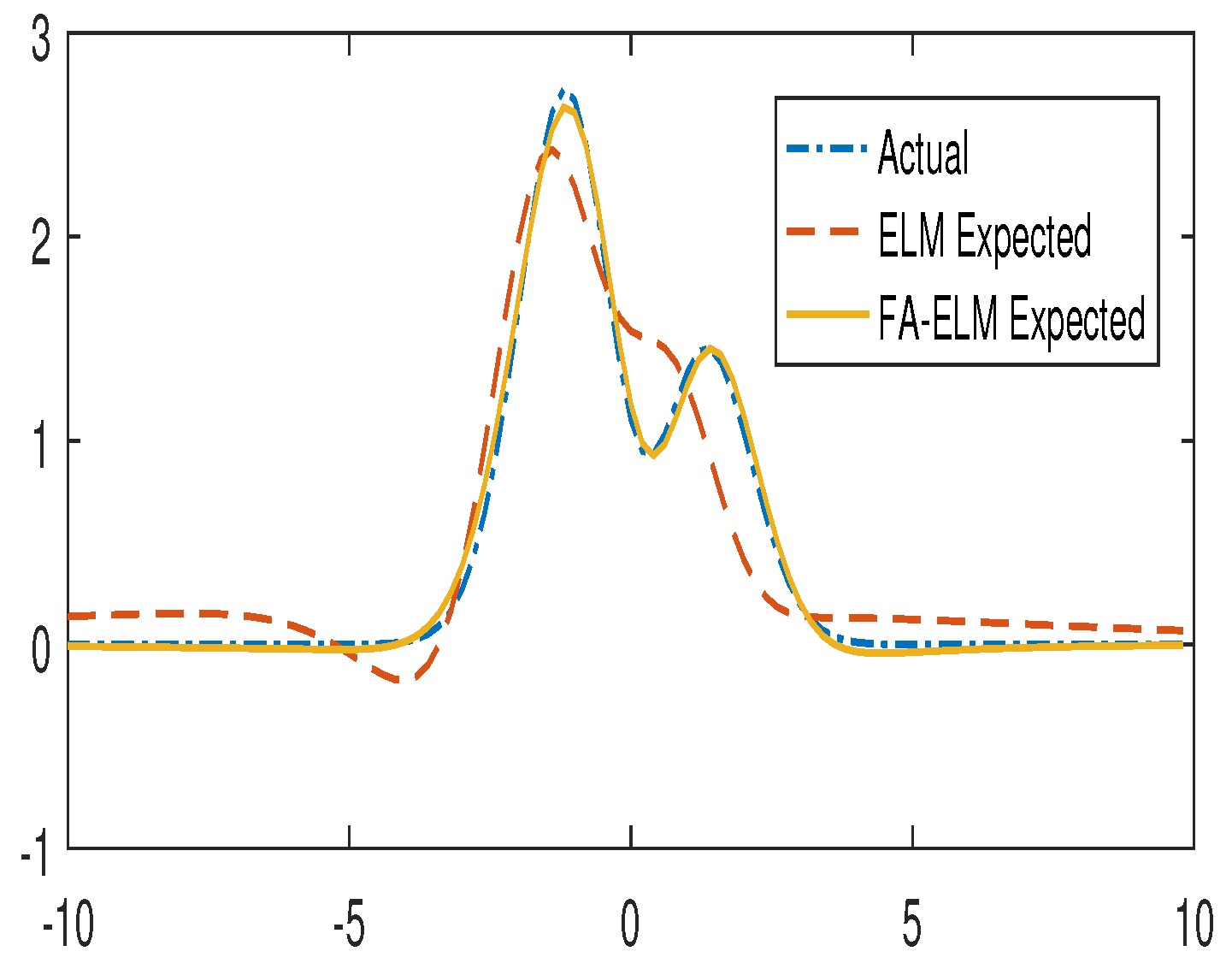
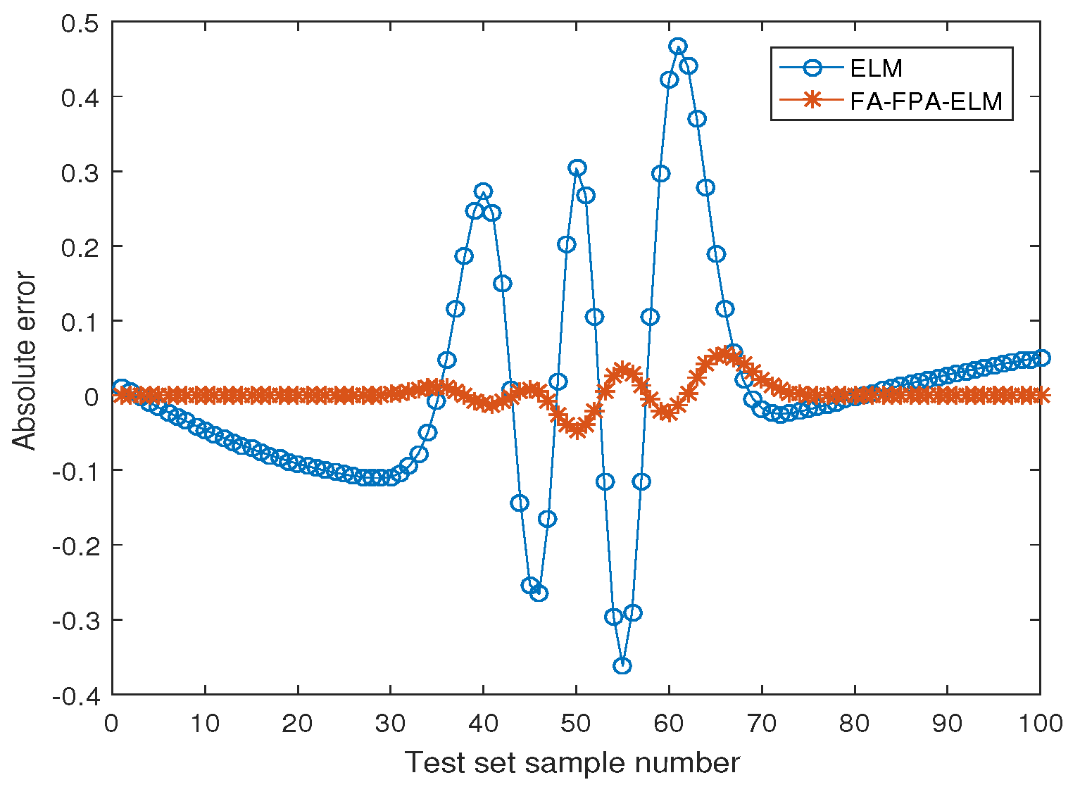
It can be discovered from Table 3 that when the hidden layer node is fixed, as the quantity of iterations increases, the training time also gradually increases, and the training error and test error decrease. When iterations reach a certain value, the test error decreases slowly. Table 4 demonstrates that with the growth of hidden layer nodes, the RMSE of FA-FPA-ELM and ELM gradually decreases. The training RMSE of the FA-FPA-ELM algorithm reaches 0.582, and only 5 hidden layer nodes are required, while the training RMSE of the ELM reaches 0.0561, which requires 20. In other words, when the two algorithms obtain almost the same training RMSE, the quantity of hidden nodes required by the new algorithm is a quarter of that of ELM. Combining Table 3 and Table 4, the maximum quantity of iterations of FA-FPA-ELM is set to 100, and the hidden layer node is 5. The fitting of ELM and FA-FPA-ELM algorithm to test function f ( x ) is shown in Figure 3. The absolute error of the two algorithms is shown in Figure 4.
It is not difficult to see that when the hidden nodes is 5, the approximation effect of FA-FPA-ELM algorithm is better than the ELM algorithm, and the absolute test error is smaller.
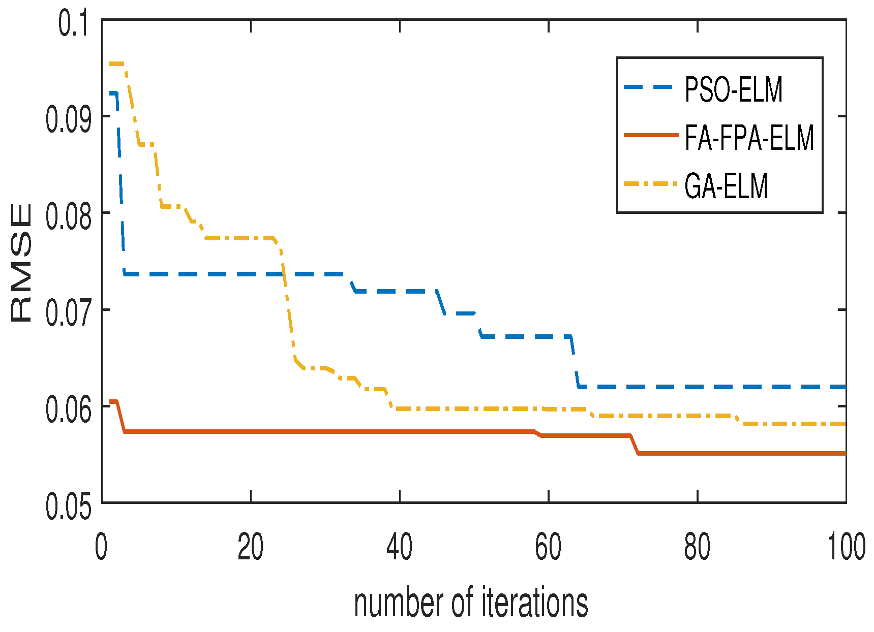
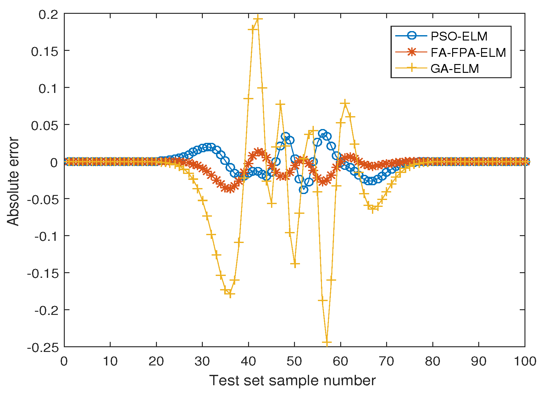
Next, we compare the approximation property of the basic ELM, FA-ELM, FPA-ELM, GA-ELM, PSO-ELM and FA-FPA-ELM algorithms. In order to ensure a fair comparison, the same population size and maximum iteration number should be used. The population size N = 10 and maximum iteration number M a x g e n = 100 have been used for these five algorithms for optimizing the ELM. FA-ELM, FPA-ELM and FA-FPA-ELM selected parameters are consistent with the above. For GA-ELM, a crossover rate of p c r o s s o v e r = 0.95 and a mutation rate of p m u t a t i o n = 0.05 are used. For PSO-ELM, an inertia weight w = 0.7 is used, and its two learning parameters c 1 = c 2 are set as 1.5. We run 30 simulation experiments on each of the six algorithms, and then give the experiment results in Table 5. Figure 5 gives the iteration curves of the three optimization algorithms (GA-ELM, PSO-ELM and FA-FPA-ELM). Figure 6 shows the absolute error of the three algorithms (GA-ELM, PSO-ELM and FA-FPA-ELM). It shown that GA, PSO and FA-FPA can effectively optimize the input parameters of ELM, and the approximation effect of FA-FPA-ELM is best by comparing the performance of the five algorithms, but the training time is longer.

5.2. Iris Classification Problem

Next, we verify the classification performance of ELM, FA-ELM, FPA-ELM, GA-ELM, PSO-ELM and FA-FPA-ELM algorithms, using the iris data set of the UCI database. Iris is a data set for multivariate analysis, it contains 150 rows of data, each row of data contains 4 attributes, divided into 3 categories. The four attributes are petal length, petal width, calyx length and calyx width. These properties are used to predict the species of iris (Setosa, Versicolour, Virginica). Among them, there is a linear relationship between the length and width of petals and the type of iris, and there is a nonlinear relationship between the length and width of sepals and the type of iris. Stochastic method is used here to generate training sets and test sets, the quantity of training samples is 100, and the rest are testing samples. For FA, FPA and FA-FPA, a step factor of α = 0.25 , a maximum attraction of β 0 = 0.2 , an absorption coefficient of light intensity λ = 1 and the initial value of the conversion probability p = 0.8 are used. For PSO-ELM, an inertia weight w = 0.7 is used, and its two learning parameters c 1 = c 2 are set as 1.5. For GA-ELM, a crossover rate of p c r o s s o v e r = 0.95 and a mutation rate of p m u t a t i o n = 0.05 are used. The above three algorithms for optimizing ELM parameters have a population size of 15 and a maximum number of iterations of 100. The fitness function is the accuracy of training samples, and the quantity of hidden layer neurons is 5. Sigmoid function is the activation function of the six algorithms. For the iris classification problem, it can be seen from Figure 7 that when optimizing the ELM parameters, the FA-ELM algorithm is unstable and will lead to a local optimal. The improved FA-FPA-ELM algorithm can jump out of the local optimal solution and accelerate the convergence speed of the FPA-ELM algorithm. The iteration curves of the three optimization algorithms (GA-ELM, PSO-ELM and FA-FPA-ELM) are presented in Figure 8. Table 6 shows the training time, testing time, training accuracy and test accuracy of the six algorithms, respectively.
It is obvious from Figure 8 that when the number of iterations is less than 40, the FA-FPA-ELM algorithm finds the optimal weights and thresholds, while the PSO-ELM algorithm finds the optimal parameters when the number of iterations is greater than 80. When the number of iterations is 100, the accuracy of FA-FPA-ELM and PSO-ELM is greater than that of GA-ELM algorithm. Table 6 shows that GA-ELM, FA-ELM, FPA-ELM, PSO-ELM and FA-FPA-ELM can effectively optimize the parameters and improve the algorithm classification accuracy. FA-FPA-ELM algorithm has the highest accuracy and better classification property than the other five algorithms, but it requires the longest training time.

5.3. Personal Credit Rating

With the development of the financial industry, banks have gradually established a corporate credit evaluation system. The evaluation methods of personal credit are mainly divided into qualitative evaluation and quantitative evaluation. Qualitative evaluation is mainly based on the subjective judgment of credit officers. Quantitative evaluation is based on individual customer data and analysis using tools such as score cards and credit scoring models. The following uses a personal customer credit evaluation method to classify all customers into two categories, only distinguishing good and bad situations. The personal credit evaluation uses a data set from the German credit database compiled by Professor Hans Hofmann, which contains 1000 customers’ data, each customer containing 20 attributes, and gives a mark of good or bad credit. Among them, each customer’s 20 attributes include 7 numeric attributes and 13 category attributes. The numeric attributes include age, bank deposits, account duration, loan amount, installment payment as a percentage of monthly income, current residence years and number of dependents. Category attributes include current account status, loan history status, loan use, deposit status, working hours, personal status, security deposit, property, other installment plans, housing status, working status, telephone number and whether it is a foreign worker. Next, we will use the newly proposed FA-FPA-ELM algorithm to evaluate user credit and compare it with the traditional ELM, FA-ELM, FPA-ELM, GA-ELM and PSO-ELM algorithms. The parameter selection of each algorithm is the same as the iris classification problem. The training set and the test set are randomly generated, the number of training sets is 700, and the number of test sets is 300. For the personal credit rating problem, it can be seen from Figure 9 that when the ELM parameters are optimized, the FA-ELM algorithm will oscillate in the iterative process and fall into a local optimum. The improved FA-FPA-ELM algorithm is relatively stable, and it has better classification accuracy. Figure 10 shows the iterative curve of GA-ELM, PSO-ELM and FA-FPA-ELM algorithm optimization. Table 7 shows the training time, testing time, training accuracy and test accuracy of the six algorithms, respectively.
Figure 10 shows that FA-FPA-ELM has the fastest convergence speed. When the number of iterations is 100, the accuracy of FA-FPA-ELM and PSO-ELM is greater than that of GA-ELM algorithm. Table 7 shows that FA-ELM, FPA-ELM, GA-ELM, PSO-ELM and FA-FPA-ELM can improve the algorithm classification accuracy. FA-FPA-ELM algorithm has the highest classification accuracy. As a result that FA-FPA-ELM requires two intelligent optimizations, it takes longer training time than FA-ELM, FPA-ELM, GA-ELM and PSO-ELM algorithms, but has a higher accuracy rate.

6. Conclusions

In this paper, our goal was to optimize the weights and thresholds of the ELM algorithm, because FA has a good global optimization ability, and FPA has a local optimization ability. Therefore, we first use the FA-ELM algorithm to get better weights and thresholds, and then use it as the initial weights and thresholds of the FPA-ELM algorithm. This new algorithm combines the advantages of ELM and FA-FPA, with simple parameter adjustment, global optimality and strong generalization ability. When fitting a nonlinear function, the RMSE and MAE of FA-FPA-ELM are better than the traditional ELM algorithm, indicating that the algorithm after optimizing the weight and threshold of ELM has a better approximation effect. In the iris classification and personal credit evaluation experiments, when the hidden node is set to 5 and the activation function is sigmoid, the classification performance of the FA-FPA-ELM algorithm is better than the traditional ELM, FA-ELM, FPA-ELM, GA-ELM and PSO-ELM, but because the FA-FPA-ELM algorithm needs to search for the optimal weights and thresholds twice, the training time is the longest. The above experiment results show that the new algorithm only needs fewer hidden layer nodes to achieve better approximation and classification results. In the future, we consider applying FA-FPA-ELM algorithm to practical engineering problems and comparing it with a wider range of algorithms.

Author Contributions

Software, L.N. and Q.K.; supervision, Q.F.; writing—original draft preparation, T.L.; writing—review and editing, Q.F. All authors have read and agreed to the published version of the manuscript.

Funding

This research was funded by Special Science Research Plan of the Education Bureau of Shaanxi Province of China (No. 18JK0344) and The 65th China Postdoctoral Science Foundation (No. 2019M652837).

Acknowledgments

We are grateful to the editor and reviewers for their insightful comments.

Conflicts of Interest

The authors declare no conflict of interest.

References

  1. Liu, D.; Baskett, W.; Beversdorf, D.Q.; Shyu, C.-R. Exploratory Data Mining for Subgroup Cohort Discoveries and Prioritization. IEEE J. Biomed. Health Inform. 2019, 24, 1456–1468. [Google Scholar] [CrossRef] [PubMed]
  2. Tsuruoka, Y. Deep Learning and Natural Language Processing. Brain Nerve 2019, 71, 45–55. [Google Scholar] [PubMed]
  3. Yasin, I.; Drga, V.; Liu, F.; Demosthenous, A.; Meddis, R. Optimizing Speech Recognition Using a Computational Model of Human Hearing: Effect of Noise Type and Efferent Time Constants. IEEE Access 2020, 8, 56711–56719. [Google Scholar] [CrossRef]
  4. Levene, M. Search Engines: Information Retrieval in Practice. Comput. J. 2011, 54, 831–832. [Google Scholar] [CrossRef]
  5. Fan, Q.; Zurada, J.M.; Wu, W. Convergence of Online Gradient Method for Feedforward Neural Networks with Smoothing L1/2 Regularization Penalty. Neurocomputing 2014, 131, 208–216. [Google Scholar] [CrossRef]
  6. Ruck, D.W.; Rogers, S.K. Comparative analysis of backpropagation and the extended Kalmanfilter for training multilayer perceptrons. IEEE Trans. Pattern Anal. Mach. Intell. 1992, 14, 686–691. [Google Scholar] [CrossRef]
  7. Li, J.; Cheng, J.-H.; Shi, J.-Y.; Huang, F. Brief Introduction of Back Propagation (BP) Neural Network Algorithm and Its Improvement. Comput. Sci. Inf. Eng. 2012, 169, 553–558. [Google Scholar]
  8. Sanz, J.; Perera, R.; Huerta, C. Fault diagnosis of rotating machinery based on auto-associative neural networks and wavelet transforms. J. Sound Vibr. 2007, 302, 981–999. [Google Scholar] [CrossRef]
  9. Yingwei, L.; Sundararajan, N.; Saratchandran, P. Performance evaluation of a sequential minimal radial basis function (RBF) neural network learning algorithm. IEEE Trans. Neural Netw. 1998, 9, 308–318. [Google Scholar] [CrossRef]
  10. Beltran-Perez, C.; Wei, H.-L.; Rubio-Solis, A. Generalized Multiscale RBF Networks and the DCT for Breast Cancer Detection. Intern. J. Auto Comput. 2020, 17, 55–70. [Google Scholar] [CrossRef]
  11. Pfister, T.; Simonyan, K.; Charles, J.; Zisserman, A. Deep Convolutional Neural Networks for Efficient Pose Estimation in Gesture Videos. Asian Conf. Comput. Vis. 2014, 9003, 538–552. [Google Scholar]
  12. Huang, G.-B.; Zhu, Q.-Y.; Siew, C.-K. Extreme learning machine: A new learning scheme of feedforward neural networks. IEEE Intern. J. Conf. Neural Netw. 2004, 2, 985–990. [Google Scholar]
  13. Huang, G.-B.; Zhu, Q.-Y.; Siew, C.-K. Extreme learning machine: Theory and applications. Neurocomputing 2006, 70, 489–501. [Google Scholar] [CrossRef]
  14. Huang, G.-B. Learning capability and storage capacity of two hidden-layer feedforward networks. IEEE Trans. Neural Netw. 2003, 14, 274–281. [Google Scholar] [CrossRef] [Green Version]
  15. Huang, G.-B.; Chen, L.; Siew, C.-K. Universal approximation using incremental constructive feedforward networks with random hidden nodes. IEEE Trans. Neural Netw. 2006, 17, 879–892. [Google Scholar] [CrossRef] [Green Version]
  16. Fan, Q.; Wu, W.; Zurada, J.M. Convergence of Batch Gradient Learning with Smoothing Regularization and Adaptive Momentum for Neural Networks. SpringerPlus 2016, 5, 1–17. [Google Scholar] [CrossRef] [Green Version]
  17. Yu, D.; Deng, L. Efficient and effective algorithms for training single-hidden-layer neural networks. Pattern Recognit. Lett. 2012, 33, 554–558. [Google Scholar] [CrossRef]
  18. Fan, Q.; Liu, T. Smoothing L0 Regularization for Extreme Learning Machine. Math. Probl. Eng. 2020, 2020, 9175106. [Google Scholar] [CrossRef]
  19. Fan, Q.; Niu, L.; Kang, Q. Regression and Multiclass Classification Using Sparse Extreme Learning Machine via Smoothing Group L1/2 Regularizer. IEEE Access 2020, 8, 191482–191494. [Google Scholar] [CrossRef]
  20. Ding, J.; Chen, G.; Yuan, K. Short-Term Wind Power Prediction Based on Improved Grey Wolf Optimization Algorithm for Extreme Learning Machine. Processes 2020, 8, 109. [Google Scholar] [CrossRef] [Green Version]
  21. Nabipour, N.; Mosavi, A.; Baghban, A.; Shamshirband, S.; Felde, I. Extreme Learning Machine-Based Model for Solubility Estimation of Hydrocarbon Gases in Electrolyte Solutions. Processes 2020, 8, 92. [Google Scholar] [CrossRef] [Green Version]
  22. Salam, M.A. FPA-ELM Model for Stock Market Prediction. Intern. J. Adv. Res. Comput. Sci. Sof. Eng. 2015, 5, 1050–1063. [Google Scholar]
  23. Zhu, Q.Y.; Qin, A.K.; Suganthan, P.N. Evolutionary extreme learning machine. Pattern Recognit. 2005, 38, 1759–1763. [Google Scholar] [CrossRef]
  24. Ling, Q.L.; Han, F. Improving the Conditioning of Extreme Learning Machine by Using Particle Swarm Optimization. Intern. J. Digit. Cont. Techn. Appl. 2012, 6, 85–93. [Google Scholar]
  25. Alexandre-Cortizo, E.; Cuadra, L.; Salcedo-Sanz, S.; Pastor-Sánchez, Á.; Casanova-Mateo, C. Hybridizing Extreme Learning Machines and Genetic Algorithms to select acoustic features in vehicle classification applications. Neurocomputing 2015, 152, 58–68. [Google Scholar] [CrossRef]
  26. Wu, L.; Zhou, H.; Ma, X.; Fan, J.; Zhang, F. Daily reference evapotranspiration prediction based on hybridized extreme learning machine model with bio-inspired optimization algorithms: Application in contrasting climates of China. J. Hydrol. 2019, 577. [Google Scholar] [CrossRef]
  27. Alam, D.; Yousri, D.; Eteiba, M. Flower Pollination Algorithm based solar PV parameter estimation. Energy Convers. Manag. 2015, 101, 410–422. [Google Scholar] [CrossRef]
  28. Bekdaş, G.; Nigdeli, S.M.; Yang, X.-S. Sizing optimization of truss structures using flower pollination algorithm. Appl. Sof. Comput. 2015, 37, 322–331. [Google Scholar] [CrossRef]
  29. Abdelaziz, A.; Ali, E.; Elazim, S.A. Flower Pollination Algorithm and Loss Sensitivity Factors for optimal sizing and placement of capacitors in radial distribution systems. Int. J. Electr. Power Energy Syst. 2016, 78, 207–214. [Google Scholar] [CrossRef]
  30. Fister, L.; Yang, X.S.; Brest, J. A comprehensive review of firefly algorithms. Swarm Evol. Comput. 2013, 13, 34–46. [Google Scholar] [CrossRef] [Green Version]
  31. Gandomi, A.H.; Yang, X.-S.; Alavi, A.H. Mixed variable structural optimization using Firefly Algorithm. Comput. Struct. 2011, 89, 2325–2336. [Google Scholar] [CrossRef]
  32. Coelho, L.D.S.; Mariani, V.C. Improved firefly algorithm approach applied to chiller loading for energy conservation. Energ. Build. 2013, 59, 273–278. [Google Scholar] [CrossRef]
  33. Xia, X.; Gui, L.; He, G.; Xie, C.; Wei, B.; Xing, Y.; Wu, R.; Tang, Y. A hybrid optimizer based on firefly algorithm and particle swarm optimization algorithm. J. Comput. Sci. 2018, 26, 488–500. [Google Scholar] [CrossRef]
  34. Yang, X.-S.; Hosseini, S.S.S.; Gandomi, A.H. Firefly Algorithm for solving non-convex economic dispatch problems with valve loading effect. Appl. Soft Comput. 2012, 12, 1180–1186. [Google Scholar] [CrossRef]
  35. Konak, A.; Coit, D.W.; Smith, A.E. Multi-objective optimization using genetic algorithms: A tutorial. Reliab. Eng. Syst. Saf. 2006, 91, 992–1007. [Google Scholar] [CrossRef]
  36. Karakatič, S.; Podgorelec, V. A survey of genetic algorithms for solving multi depot vehicle routing problem. Appl. Sof. Comput. 2015, 27, 519–532. [Google Scholar] [CrossRef]
  37. Trelea, I.C. The particle swarm optimization algorithm: Convergence analysis and parameter selection. Inform. Process. Lett. 2003, 85, 317–325. [Google Scholar] [CrossRef]
  38. Tasgetiren, M.F.; Liang, Y.C.; Sevkli, M.; Gencyilmaz, G. A particle swarm optimization algorithm for makespan and total flowtime minimization in the permutation flowshop sequencing problem. Eur. J. Oper. Res. 2007, 177, 1930–1947. [Google Scholar] [CrossRef]
  39. Li, S.-A.; Hsu, C.-C.; Wong, C.-C.; Yu, C.-J. Hardware/software co-design for particle swarm optimization algorithm. Inform. Sci. 2011, 181, 4582–4596. [Google Scholar] [CrossRef]
  40. Yang, X.-S.; Karamanoglu, M.; He, X. Flower pollination algorithm: A novel approach for multiobjective optimization. Eng. Optimiz. 2013, 46, 1222–1237. [Google Scholar] [CrossRef] [Green Version]
  41. Liu, W.; Luo, F.; Liu, Y.; Ding, W. Optimal Siting and Sizing of Distributed Generation Based on Improved Nondominated Sorting Genetic Algorithm II. Processes 2019, 7, 955. [Google Scholar] [CrossRef] [Green Version]
  42. Han, Z.; Zhang, Q.; Shi, H.; Zhang, J. An Improved Compact Genetic Algorithm for Scheduling Problems in a Flexible Flow Shop with a Multi-Queue Buffer. Processes 2019, 7, 302. [Google Scholar] [CrossRef] [Green Version]
  43. Pavlyukevich, I. Lévy flights, non-local search and simulated annealing. J. Comput. Phys. 2007, 226, 1830–1844. [Google Scholar] [CrossRef] [Green Version]
  44. Yang, X.S. Flower Pollination Algorithm for Global Optimization. Unconv. Comput. Natural. Comput. 2012, 7445, 240–249. [Google Scholar]
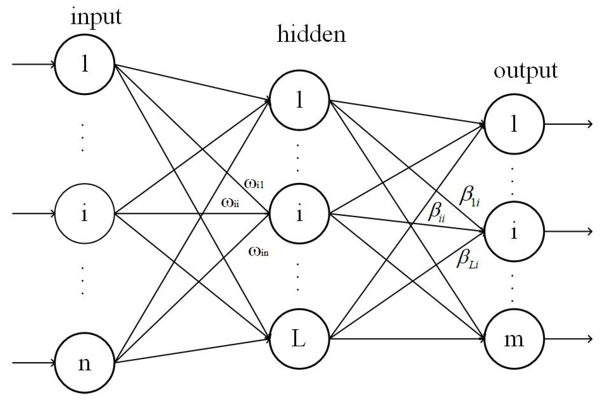
Figure 1. The network structure of extreme learning machine.
Processes 08 01583 g001
Figure 2. Comparison of RMSE in FPA-ELM, FA-ELM and FA-FPA-ELM algorithms on a nonlinear function.
Processes 08 01583 g002
Figure 3. Prediction of the ELM and FA-FPA-ELM algorithm for a nonlinear function.
Processes 08 01583 g003
Figure 4. Comparison of prediction errors for a nonlinear function.
Processes 08 01583 g004
Figure 5. Comparison of iteration curves of a nonlinear function.
Processes 08 01583 g005
Figure 6. Comparison of prediction errors for a nonlinear function.
Processes 08 01583 g006
Figure 7. Comparison of accuracy in FPA-ELM, FA-ELM and FA-FPA-ELM algorithms on the iris data set.
Processes 08 01583 g007
Figure 8. Comparison of iteration curves of the iris data set.
Processes 08 01583 g008
Figure 9. Comparison of accuracy in FPA-ELM, FA-ELM and FA-FPA-ELM algorithms on the personal credit rating data set.
Processes 08 01583 g009
Figure 10. Comparison of iteration curves of the personal credit rating data set.
Processes 08 01583 g010
Table 1. Steps to achieve firefly-based adaptive flower pollination algorithm (FA-FPA).
step 1: Initialize algorithm parameters, and set loop termination condition;
step 2: Stochastically initialize the position of fireflies, and calculate the target function value of each individual;
step 3: Use formulas (11) and (13) to determine the direction of movement of individuals;
step 4: Update the individual’s spatial position according to formulas (14);
step 5: Calculate the fitness function value of each individual on the grounds of the updated individual’s position;
step 6: Generate σ randomly, calculate the conversion probability p according to formulas (10);
step 7: Generate r a n d [ 0 , 1 ] randomly, if p > r a n d , then conduct a global search according to formula (9);
step 8: If p r a n d , then conduct a local search according to formula (8);
step 9: Calculate the fitness function value of each pollen to find the current optimal solution;
step 10: Judge whether the loop termination condition is met. If not, go to Step 3; if satisfied, go to Step 6;
step 11: Output the result, the algorithm ends.
Table 2. Steps to achieve FA-FPA-extreme learning machine (ELM).
step 1: Initialize algorithm parameters, and set loop termination condition;
step 2: Encode ELM input parameters into individual pollen according to formula (16);
step 3: Normalize the data according to formula (15) and randomly initialize individual positions;
step 4: Use the formula (19) to calculate the fitness function value of each individual;
step 5: Use FA to get the initial population, Generate σ randomly, calculate the conversion probability p;
step 6: Generate r a n d [ 0 , 1 ] randomly, if  p > r a n d , then conduct a global search;
step 7: If p r a n d , then conduct a local search in the light of formula (8);
step 8: Calculate the fitness value of each pollen according to formula (19) and find the current optimal solution;
step 9: Judge whether the loop termination condition is met. If not, go to Step 5; if satisfied, go to Step 10;
step 10: Decode individual pollen into ELM input parameters for network training;
step 11: Output the result, the algorithm ends.
Table 3. The impact of the iteration number on FA-FPA-ELM.
Maximum Iteration NumberTime (s)TrainingTesting
TrainingTestingRMSEMAERMSEMAE
50.61770.00060.06480.05460.02870.0175
100.96320.00060.06380.05340.02620.0127
201.61820.00060.06070.05080.02060.0097
503.63090.00060.05890.04970.01410.0078
1007.05240.00070.05830.05030.01220.0063
50034.08950.00080.05790.05100.01020.0052
Table 4. The impact of hidden layer nodes on ELM and FA-FPA-ELM.
Hidden NodesTraining Time (s)Training (RMSE)Testing (RMSE)
ELMFA-FPA-ELMELMFA-FPA-ELMELMFA-FPA-ELM
20.00767.83630.51040.10410.52590.0871
50.00907.67540.28920.05820.28070.0108
100.00868.21320.07110.05760.03930.0104
150.00948.92310.05660.05650.01200.0113
200.01159.55750.05610.05600.01250.0128
Table 5. Comparison of RMSE in ELM, FA-ELM, FPA-ELM, genetic algorithm (GA)-ELM, particle swarm optimization (PSO)-ELM and FA-FPA-ELM algorithms on a nonlinear function.
Learning
Algorithms
Training Time
(s)
Testing Time
(s)
Training
(RMSE)
Testing
(RMSE)
ELM0.01190.00170.23150.2274
FA-ELM3.23710.00080.06050.0194
FPA-ELM3.33840.00110.05620.0102
GA-ELM5.33920.00140.07370.0459
PSO-ELM4.88090.00320.06210.0221
FA-FPA-ELM9.57870.00450.05800.0099
Table 6. Comparison of accuracy in ELM, FA-ELM, FPA-ELM, GA-ELM, PSO-ELM and FA-FPA-ELM algorithms on the iris data set.
Learning
Algorithms
Training Time
(s)
Testing Time
(s)
Training
Accuracy
Testing
Accuracy
ELM0.00100.005184.60%85.80%
FA-ELM4.57690.000385.20%84.60%
FPA-ELM4.73290.000397.60%95.60%
GA-ELM4.94400.004296.30%93.60%
PSO-ELM4.88760.003496.40%94.80%
FA-FPA-ELM9.64650.011298.20%97.40%
Table 7. Comparison of accuracy in ELM, FA-ELM, FPA-ELM, GA-ELM, PSO-ELM and FA-FPA-ELM algorithms on the personal credit rating data set.
Learning
Algorithms
Training Time
(s)
Testing Time
(s)
Training
Accuracy
Testing
Accuracy
ELM0.00100.005370.37%70.07%
FA-ELM52.01750.003271.85%70.20%
FPA-ELM52.76290.014173.71%73.50%
GA-ELM70.78810.010172.86%72.13%
PSO-ELM64.86980.006574.20%73.73%
FA-FPA-ELM123.33320.005575.09%76.80%
Publisher’s Note: MDPI stays neutral with regard to jurisdictional claims in published maps and institutional affiliations.