Modeling and Experimental Validation of Compression and Storage of Raw Biogas

Abstract

A significant challenge in sustainability and development of energy systems is connected with limited diversity and availability of fuels, especially in rural areas. A potential solution to this problem is compression, transport, and storage of raw biogas, that would increase diversity and availability of energy sources in remote areas. The aim of this study was to perform experimental research on raw biogas compression concerning biogas volume that can be stored in a cylinder under the pressure of 20 MPa and to compare obtained results with numerical models used to describe the state of gas at given conditions. Results were used to determine the theoretical energy content of raw biogas, assuming its usage in CHP systems. In the study, six compression test runs were conducted on-site in an agricultural biogas plant. Compression time, pressure as well as gas volume, and temperature rise were measured for raw biogas supplied directly from the digester. Obtained results were used to evaluate raw biogas compressibility factor Z and were compared with several equations of state and numerical methods for calculating the Z-factor. For experimental compression cycles, a theoretical energy balance was calculated based on experimental results published elsewhere. As a result, gas compressibility factor Z for storage pressure of 20 MPa and a temperature of 319.9 K was obtained and compared with 6 numerical models used for similar gases. It was shown that widely known numerical models can predict the volume of compressed gas with AARE% as low as 4.81%. It was shown that raw biogas supplied directly from the digester can be successfully compressed and stored in composite cylinders under pressure up to 20 MPa. This proposes a new method to utilize raw biogas in remote areas, increasing the diversity of energy sources and increasing the share of renewable fuels worldwide.

1. Introduction

The modern energy sector faces numerous challenges connected with the increasing electricity demand. At the same time, there is a growing need for an increase in the share of renewables and improvement in energy source diversity. Renewable energy usage in Europe reached a share of 17% in the gross final energy consumption in 2015, and the projections show that it will exceed the target of 20% in 2020 [1]. Gaseous fuels are of great importance, and their consumption is increasing, based on current trends. In Poland, the majority of natural gas (NG) is imported (~78%), which is connected with limited capabilities to extract this gas nationwide. Despite the significant increase in renewables usage in electricity generation, there is a very limited alternative for compressed gas distribution, similar to compressed natural gas (CNG), which can be supplied in areas lacking connection to the natural gas grid.

Biogas (being a mixture of 45–74% CH₄, mostly with 25–45% CO₂) is regarded as a renewable energy source that becomes a highly effective alternative for fossil fuels [2,3,4]. It can be obtained through anaerobic digestion of biomass, landfill gas recovery, sewage sludge, and biomass thermal processing. Similar to other biofuels, biogas has several benefits for the circular economy and sustainability. At first, there is plenty of biomass to be valorized both worldwide and in Europe. According to [5], there were 17,783 biogas plants in Europe in 2017, which produced biogas mostly in anaerobic digestion of agricultural residues [1]. Biodegradable waste, such as, for example, biowaste from households is a valuable source of energy, can be directly valorized into high-quality fuel [6]. Biogas can be utilized in many different forms, such as fuel for vehicles [2,7,8] or in heat generation. Still, there are other, more economically justified technologies for obtaining heat with other renewables such as wood chips, straw and pellets [9]. In Europe, most biogas obtained in anaerobic digestors produces electricity, heat or both in combined heat and power (CHP). 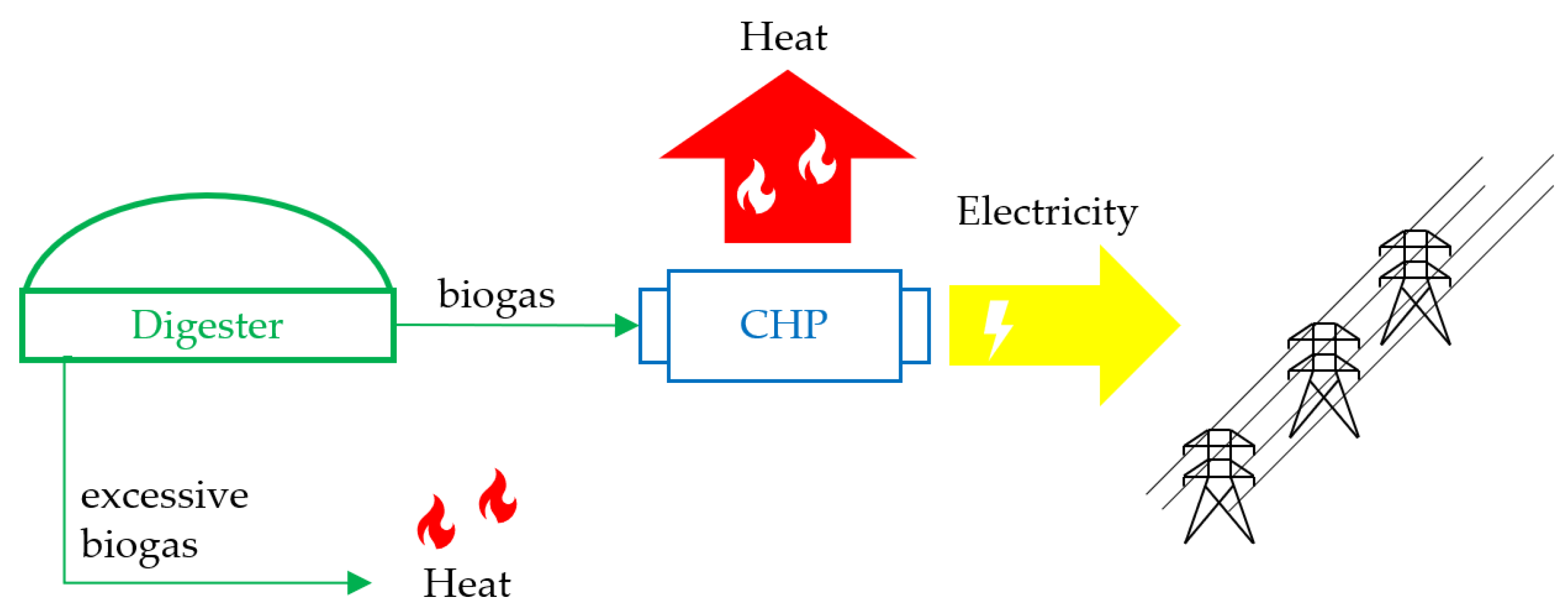In 2017, electricity generation from biogas was mostly associated with agricultural feedstock, with the only marginal share of the landfill and sewage biogas [5]. In Poland, a typical agricultural biogas plant produces biogas and generates heat and electricity in CHP on-site, selling electricity to the electric grid and supplying nearby residential dwellings in heat. This is shown in Figure 1.

Despite several advantages, such as increased efficiency compared to heat- and/or electricity-only solutions, CHP has some disadvantages, for example, limited need for heat during the summer period by most farms producing biogas in anaerobic digestion [9]. This makes CP economically reasonable only if there is a heat recipient that could benefit from heat obtained from biogas, which is very difficult, providing most biogas plants are located in rural areas. Although economic success for farm-scale biogas production depends on the scale of its production, it is not clear whether a large, centralized biogas plant is the better choice compared to smaller plants utilizing biowaste from neighboring farms [9].

The application of biogas in energy generation makes CO₂ circulate between air and fuel, which positively affects both greenhouse gas emissions and has the potential to satisfy increasing energy demand. Among different technical solutions for energy generation in CHP, the spark ignition (SI) engine is the most economically reasonable option for small-scale biogas plants, regardless of the economic value of electricity and heat produced [9]. As it was shown by Qian et al., a high amount of CO₂ in raw biogas can help to inhibit NO_x emissions, which positively contributes to greenhouse gas emissions [10]. There are numerous studies on combustion characteristics of different biogas combinations [3,6,9,10,11,12,13,14]. It was described by Jerzak et al. that co-digestion of organic municipal waste with agricultural waste could be beneficial as it increases the content of methane in the biogas from 45% to about 55–60% [6]. The increase in the concentration of methane in the biogas simultaneously causes a decrease in the concentration of CO2 in the biogas, which further reduces greenhouse gas emissions from biogas combustion. Despite those efforts, the low calorific value of biogas is one of the most important barriers to biogas development in the combined heat and power (CHP) generation [12]. According to Jørgensen et al., pure biogas is not eligible to be substituted for either liquid petroleum gas (LPG) or natural gas (NG) in commercial burners without any modification [11]. The same applies to vehicle engines, which are not suitable to be powered by raw biogas [7]. Recent advancements in biogas upgrading technologies, together with problems in the utilization of energy from CHP (mostly heat) and current opportunities for the use of biogas in the transport sector, resulting in a shift from electricity and heat production to biogas to biomethane upgrading [1]. Biogas purification, although being justified from the point of view of biogas calorific value, is often not economical [11].

An alternative solution to this problem is generating electricity and heat in areas where there is a high demand for those forms of energy. This means that biogas could be produced in diverged biogas plants and then transported to remote areas where it is needed. This is done predominately by injecting biogas to a gas grid, reducing storage costs and allowing its use at the places where it is needed [1]. For this to be possible, biogas needs to fulfill restrictive requirements regarding its composition. This requires a costly pretreatment of raw biogas to eliminate impurities in order to adopt the composition of biogas to grid distribution requirements. Moreover, it needs the biogas plant to be close to a low-pressure natural gas grid.

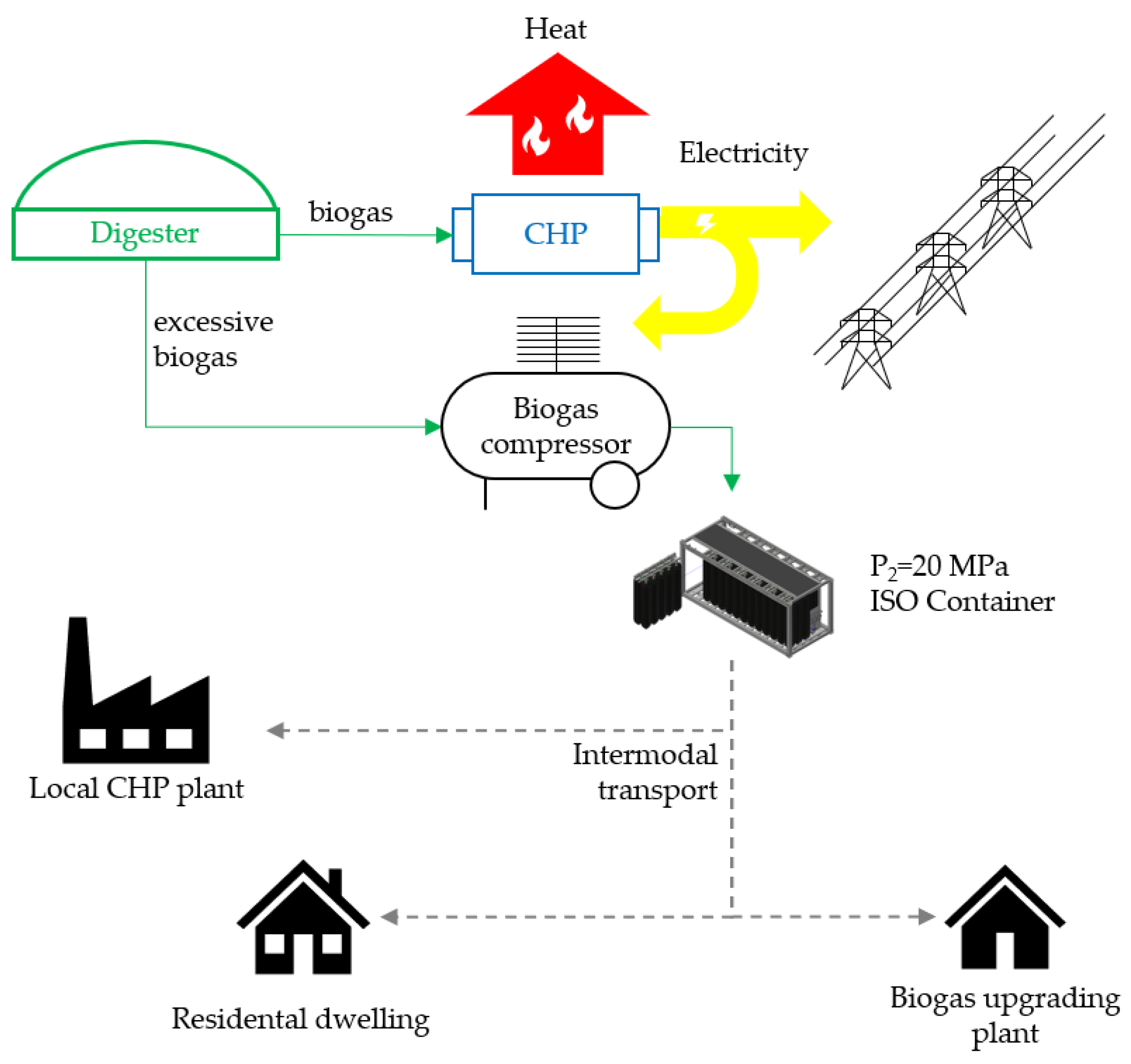
In this work, the authors propose a novel and innovative method to utilize raw agricultural biogas obtained in anaerobic digestion of agricultural waste as a mobile energy source ready to be supplied to remote areas by intermodal transport using modular gas containers. This method involves the production of raw biogas in diverged plants, its compression and distribution to isolated areas having demand for electricity and heat. Compressing biogas directly from the digester eliminates the need for investment in biogas upgrading technologies, making it less expensive to valorize biomass into gaseous fuel. Transport of compressed raw biogas to remote areas could increase the availability of biogas in areas where there is no natural gas grid, increasing the diversity of energy sources and contributing to the effective development of circular economy and sustainable energy systems. The proposed system called compressed biogas distribution system (CBDS) is presented in Figure 2.

There are published results on compression of various gaseous fuels, predominately of natural gas and biomethane [15,16,17,18,19,20,21]. Still, there is a lack of experimental data on raw biogas compression taken directly from the digester. In this research, the authors aimed to obtain experimental results of raw biogas compression and selection of the best method to describe the volume of gas in transport, which determines further development of CBDS. This work presents original and novel raw biogas compression results performed on-site in real-life conditions and compares them with widely used methods for estimating the volume of gas in transport. As a result, theoretical energy balance for CBDS is presented, including electricity and heat generation in CHP and energy demand for biogas compression.

2. Materials and Methods

In this work, experimental analysis of raw biogas compression was performed. At first, an experimental setup was prepared in a local biogas plant that involved a compressor, gas supply, pressure cylinder, and set of gauges to measure the biogas compression process. Experimental testing consisted of 6 consecutive compression test runs, in which biogas was fed directly from the digester to the pressure cylinder by the compressor. As a result, biogas was compressed to the pressure of 20 MPa.

The scope of this experimental research was to examine a volume of raw biogas that can be compressed in the pressure cylinder of known volume in a pressure range from 10 MPa to 20 MPa and to compare obtained results with numerical models used to estimate the volume of biogas in transport. The authors decided to use the above pressure range because this is a typical range in which compressed gases, e.g., compressed natural gas (CNG), are being stored [4,22]. Measured composition of biogas together with ambient temperature and pressure were used to evaluate the volume of gas in transport using various equations of state (EoS), and results were compared with experimental results obtained from each test run. For validated numerical models, the energy content of one transport of raw biogas in a given storage volume was estimated, and the amount of electric and heat energy that can be obtained in CHP was evaluated.

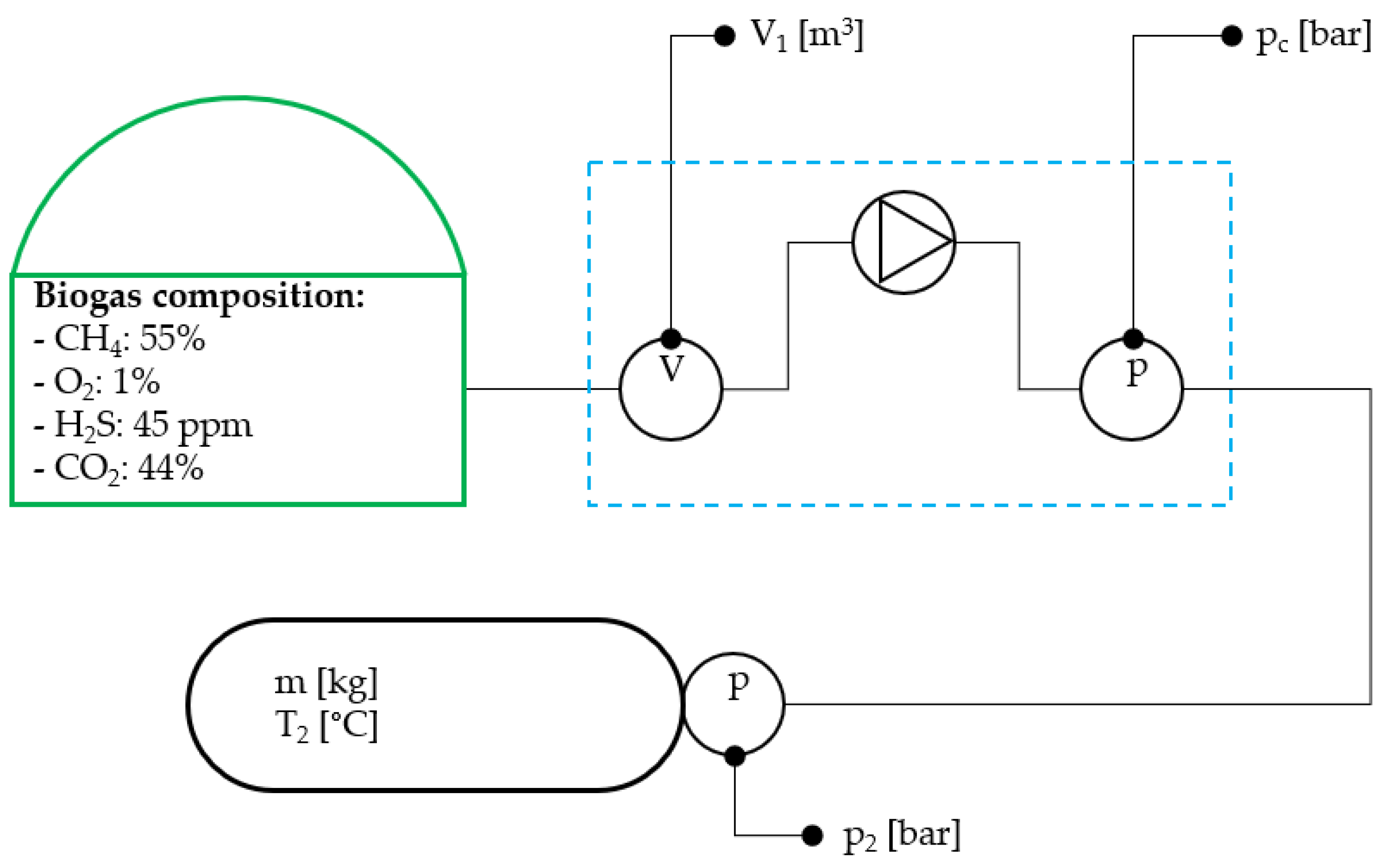
2.1. Raw Biogas Compression

In total, 6 compression cycles were performed in all of which raw biogas was taken directly from the digester and compressed to the point in which pressure in the cylinder reached 20 MPa. During each cycle, the following variables were measured:

• V₁ (volume of biogas taken by the compressor from the digester);
• p₂ (pressure of biogas inside the cylinder);
• p_c (pressure of biogas after the III stage of the compressor);
• m₂ (mass of compressed biogas).

All variables above were measured at an interval of one minute. The volume of gas in a compressed state (V₂) was equal to 0.0068 m³. As a result of measurement, V₁(t) and m₂(t) graphs were created for each test run. The molecular composition of compressed raw biogas and values of ambient temperature (T₁) and ambient pressure (p₁) are presented in

Table 1. Raw biogas composition used in experiments.

Parameter	Value	Typical Values Based on [4]
CH4,%	55%	54.73%
CO2,%	44%	34.99%
O2,%	1%	0.34%
H2S, ppm	45	99.75

. Biogas composition was provided by the biogas plant based on the measurement directly in the digester. This information is easily accessible and thus can be used in the exploitation of CBDS daily. Description of the used cylinder and biogas compressor are presented in

Table 2. Data related to ambient temperature, pressure, biogas cylinder and compressor used in experimental testing.

Parameter		Value	Description
Ambient temperature	T1	313.15 K	Temperature of anaerobic digestion in the examined biogas plant
Ambient pressure	p1	102,500 Pa	Atmospheric pressure in the day of measurements + overpressure in the digester
Volume of the compressed biogas storage cylinder	V2	0.0068 m3	The volume of water that would fill the cylinder uncompressed
Maximum filling pressure	pmax	30 MPa	-
Cylinder material	-	-	Aluminum liner, carbon wrap with glass wrap
Outer diameter of the cylinder	Dc	152.5 mm	-
Cylinder length	Lc	546 mm	-
Data Related to the Biogas Compressor Used in Experimental Research
Compressor	Aqacentrum Praha S.R.O. Trident 05 3 kW electric motor, 960 rpm
Compression stages	I stage: inlet pressure—0.7 MPa II stage: 0.7 MPa–5 MPa III stage: 5 MPa–21 MPa

.

Because experiments were performed on-site and no access to the inside of the cylinder was possible, the assumption was made that the temperature of the cylinder’s outer surface was equal to the temperature of biogas in the cylinder at a given time frame. For temperature measurement, FLIR ThermaCAM E300 was used that has a measuring range from −20 °C to +250 °C, with an accuracy of ±2 °C or ±2%, whichever is bigger. During each test run, the temperature was measured at the outer surface of the cylinder using a thermal camera, and the maximum measured temperature for a given time frame was recorded.

Additional assumptions made during compression tests were as follows:

• the volume of biogas measured at the inlet of the compressor was equal to the volume stored in the cylinder; thus, the assumption was made that the volume of gas in piping and cylinders of the compressor is equal before and after compression;
• the ambient temperature and pressure of biogas were equal to digestion parameters used in biogas plant;
• the increase of temperature of the outer surface of the cylinder was a result of increased biogas temperature through compression, not through solar heat (cylinder was protected before sunlight);
• the piping and instrumentation used in the experiment were sealed that no air could enter the cylinder during compression, which was facilitated by the pre-compression of biogas in the used cylinder before the first test run. This means the composition of compressed biogas was unchanged compared to the gas in the digester;
• during the entire compression process, it as assumed that the compressor operated at nominal power, making it possible to estimate the amount of energy used for compression;
• the composition of biogas was the same before and after all six consecutive test runs.

A scheme of a test bench used in experimental research is presented in Figure 3.

As a result of all six test runs in experimental research on compression of raw biogas, the following quantities were measured:

(a)

at an interval of 60 s:

• mass of compressed biogas, m₂(t), kg;
• pressure of biogas inside the cylinder, p₂(t), bar;
• volume of biogas taken by the compressor from the digester, V₁(t), m³;

(b)

at measured values of pressure p₂ from 100 bar to 200 bar, with an increment of 10 bar:

• temperature of the outer wall of the cylinder, T₂(t), °C.

2.2. Estimation of Z-Factor for Raw Agricultural Biogas Based on Experimental Results

From the point of view of compressed gas storage systems, it is important to know the volume of gas that can be stored in a given volume. This can be estimated using many different approaches, among which the real gas equation of state (EoS) is often used [22]. To estimate the state of gas at a given pressure and temperature, it is required to estimate gas compressibility factor Z that is used to model the behavior of gas storage systems. The real gas EoS can be written as:

$$p·V=n·R·T·Z$$

(1)

where:

p—pressure, Pa;

V—volume, m³;

n—number of moles, -;

R—universal gas constant, J·(mol·K)⁻¹;

T—temperature, K;

Z—compressibility factor, -.

Compressibility factor Z is the ratio of the actual volume occupied by gas under specific conditions to the volume occupied by the same gas treated as an ideal gas. This factor is thus a measure of the amount the real gas deviates from an ideal gas model. It is also called the gas deviation factor. To determine the gas volume in compression for the given conditions, an assumption is made that there is no gas leakage in the process; thus, the mole number before and after compression is constant (nR = const). In addition, it is assumed that gas is being compressed from ambient pressure and temperature. The above makes it possible to transform Equation (1) to the form:

$$\frac{p_1{V}_1}{T_1{Z}_1}=\frac{p_2{V}_2}{T_{2}Z}$$

(2)

where:

p₁—ambient pressure, Pa;

p₂—pressure in a compressed state, Pa;

T₁—ambient temperature, K;

T₂—temperature in a compressed state, K;

V₁—volume of gas under ambient pressure and temperature, m³;

V₂—volume of gas in a compressed state, m³;

Z₁—compressibility factor of gas under ambient pressure and temperature, -;

Z—compressibility factor in a compressed state, -.

It was assumed that in a non-compressed (ambient) state, compressibility factor Z of gaseous mixtures of CH₄/CO₂ is equal to one. This is in agreement with the results presented in [15,17,19] for gas composition given in Table 1. Solving Equation (2) for V₁ results in (for $Z_1\cong 1$):

$$V_1=\frac{p_2}{p_1}·\frac{T_1}{T_2}·V_2·\frac{1}{Z}$$

(3)

From Equation (3), to estimate the volume of gas in transport V₁ that is stored in a given volume V₂ under pressure p₂ and temperature T₂, it is required to know ambient values of pressure p₁ and temperature T₁ before compression as well as compressibility factor Z, which is dependent on p₂ and T₂ [15,17,22,23,24]. There are numerous methods on how to determine the compressibility factor for gaseous mixtures. Some of them are based on solving cubic EoS [18,22,25,26], while others concentrate on estimating compressibility factor based on critical temperature and pressure of the compressed gas [17,19,22,27].

In this study, the compressibility factor of raw biogas was calculated based on results obtained during raw biogas compression. For this purpose, the following equation was used:

$$Z=\frac{V_{ideal}}{V_1}$$

(4)

Volume V₁ was measured during compression on the flowmeter mount at the inlet of the compressor. The volume of gas treated as an ideal gas was obtained from Equation (5), which can be transformed to (6) to obtain Z-factor:

$$V_{ideal}=\frac{T_1}{T_2}·\frac{p_2}{p_1}·V_2$$

(5)

$$Z=\frac{T_1}{T_2}·\frac{p_2}{p_1}·\frac{V_2}{V_1}$$

(6)

For the results to be comparable within all six test runs, the gas temperature in the compressed state (T₂) was measured and used to formulate T(p) dependence, that was further used for all test runs providing, that the obtained function could be assumed to represent measured values of temperature at probability value smaller than 0.05. Such obtained value of temperature, denoted by T₂′, was used in Equation (7) together with measured values of p₂, p₁, T₁ and V₁ to evaluate the compressibility factor of raw biogas:

$$Z=\frac{T_1}{T_2{}^{’}}·\frac{p_2}{p_1}·\frac{V_2}{V_1}$$

(7)

As a result of this step, the compressibility factor of biogas was calculated using measured values of pressure, temperature and gas volume, and it was further used to validate numerical models used to estimate Z-factor for biogas.

2.3. Validation of Numerical Models

In order to validate obtained results, compressibility factor Z was evaluated based on the measured composition of raw biogas (Table 1) using known equations of state and empirical correlation based on results published elsewhere [17,19,22,25,26,27]. For this study, Peng–Robinson (1976), Soave–Redlich–Kwong (1972) and Redlich–Kwong (1949) cubic equations of state were used [25,26] as well as empirical correlations based on results published by Sanjari and Lay (2012), Beggs and Brill (1973) and Eilerts (1948) [19,22,27]. Selection of methods was performed based on the range of applicability of each method, providing it is suitable to calculate Z-factor for gases having high CO₂ content. Parameters used for the estimation of the Z-factor are shown in

Table 3. Data used in the calculation for Z-factor for raw biogas constituents, based on [28].

Constituent	yi	kij	CH4	CO2	O2	ω	Tc (K)	Pc (MPa)	Molar Mass
CH4	0.55	CH4	-	0.996	-	0.011	190.4	4.60	16.04
CO2	0.44	CO2	0.996	-	-	0.239	304.1	7.38	44.01
O2	0.01	O2	-	-	-	0.025	154.6	5.04	32.00

.

Peng–Robinson (1976) and Soave–Redlich–Kwong (1972) EoS are the most widely used to estimate parameters of compressed gases, including mixtures of CH₄ with CO₂ [19,20]. Those equations, along with Redlich–Kwong (1949) EoS, are referred to in terms of the Z-factor as cubic equations of state and are in the form:

$$Z^3+A_1{Z}^2+A_{2}Z+A_3=0$$

(8)

Formulas for the determination of coefficients A₁, A₂ and A₃ depend on the applied EoS and mixing rules, which are required by both PR and SRK EoS. The selection of mixing rules depends on the composition of the compressed gas. In this study, Van Der Waals mixing rules were used for both PR and SRK EoS, as suggested in [24]. Binary interaction coefficients k_ij used in those mixing rules are typically obtained by experimental testing. For the purpose of this work, they were assumed based on published data.

A different approach to evaluate the gas compressibility factor was proposed by [19,22,29]. Standing and Katz, taking into account a theory of corresponding states for calculating the Z-factor, have developed a chart, known as the S-K Chart, which is widely used for natural gas [15,17,22] and biogas [4,30]. This method of determination of gas compressibility factor for mixtures is based on the calculation of pseudoreduced values of pressure and temperature, p_pr and T_pr according to formulas:

$$T_{pr}=\frac{T}{{{\displaystyle \sum }}_{i=1}^n{y}_i·T_{ci}}$$

(9)

$$p_{pr}=\frac{p}{{{\displaystyle \sum }}_{i=1}^n{y}_i·p_{ci}}$$

(10)

where:

p, T—pressure and temperature at a given state of gas;

y_i—molar ratio of i-th gas constituent;

p_ci, T_ci—critical pressure and temperature of the i-th gas constituent.

Knowing p_pr and T_pr, the gas compressibility factor can be obtained either directly from the S-K Chart [29] or by substituting those values to various correlation equations, such as [17,19,27].

Another method to evaluate the gas compressibility factor is to use the method of weighing treatment, proposed by Eilerts and described in [22]. In this approach, it is required to know the composition of the analyzed gas and, for each constituent, the Z-factor for a given state. Then, by application of Equation (11), it is possible to obtain the compressibility factor of a gas mixture providing, that analyzed gas is composed of both hydrocarbon and non-hydrocarbon components [22]:

$$Z={{\displaystyle \sum }}_{\mathrm{i}=0}^{\mathrm{n}}{y}_i·Z_i$$

(11)

where:

Z_s—compression factor of a gas mixture with a given chemical composition;

y_i—mole fraction of the gas component;

Z_i—compressibility factor of gas component (mono-component gas).

This method was described as useful in the determination of the Z-factor of compressed syngas [31] and natural gas with increased N₂ content [22] and was also used in the theoretical analysis of raw biogas compression before [32].

In this paper, compressibility factors evaluated with the above-mentioned methods were used to estimate the volume of gas stored in a cylinder having volume V₂ = 0.0068 m³ and values were compared with experimental results using average relative error (ARE%), average absolute relative error (AARE%) and root mean square error (RMSE) to identify the best match, which was further used to evaluate the volume of gas in transport for designed CBDS.

2.4. Energy Content of Raw Biogas

Based on available data, the energy content of raw biogas was estimated based on [4] according to Equation (12):

$$C{w}_b=Cw·\frac{{\mathrm{CH}}_4\%·M}{22.4·100}$$

(12)

where:

$C{w}_b$—energy content in raw biogas, MJ·m⁻³;

${\mathrm{CH}}_4\%$—molar fraction of CH₄ in biogas, %;

M—molar mass of CH₄;

$Cw$—energy content of pure CH₄, MJ·m⁻³.

Substituting data from Table 1 into Equation (12) and assuming, that under standard temperature and pressure (STP, T = 273.15 K, P = 100 kPa), C_w = 35.7142 MJ/m³ [4]:

$$C{w}_b=Cw·\frac{{\mathrm{CH}}_4\%·16}{22.4·100}\cong 35.7142·y_{\mathrm{CH}4}=19.64\frac{\mathrm{MJ}}{{\mathrm{m}}^3}$$

(13)

By knowing this value, it is possible to determine the energy content of compressed biogas E_BG, MJ·m³, which is defined as (under the assumption that energy content of pure CH₄ does not change between STP and ambient conditions shown in Table 2):

$$E_{BG}=V_1·C{w}_b$$

(14)

For CHP, values of electric energy generated (E_E) and heat (E_H) can be estimated using equations:

$$E_E=E_{BG}·{\eta }_E$$

(15)

$$E_H=E_{BG}·{\eta }_H$$

(16)

where:

η_E—electric efficiency of a CHP unit;

η_H—heat efficiency of a CHP unit.

Electric energy in MJ used for compression in experimental testing was calculated using equation:

$$E_C=\frac{P_c·t_c}{1000}$$

(17)

where:

P_c—the power of an electric motor of a compressor, kW;

t_c—total compression time, s.

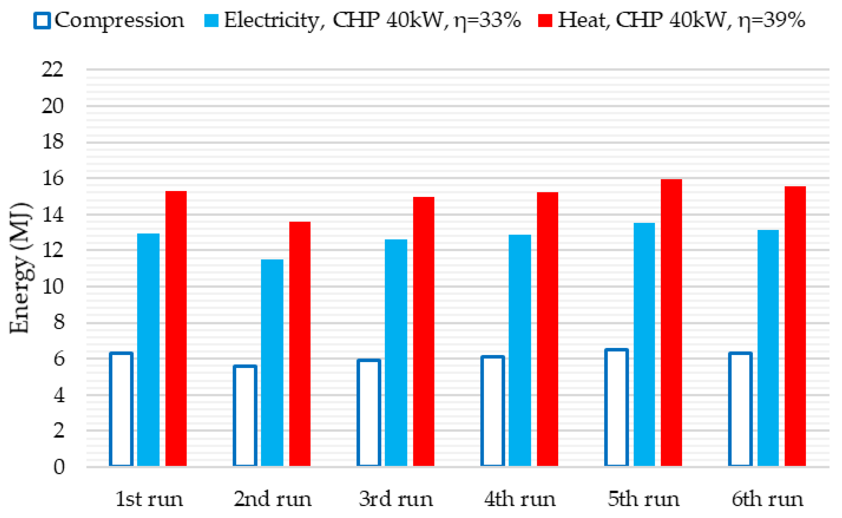
In this study, two CHP units were chosen, having installed power of 35 kW and 40 kW, respectively. Based on data published elsewhere [9], such CHP units could be installed in a relatively large farm equivalent to approximately 260 milking cows. The CHP unit with 35 kW of power has electric and heat efficiency equal to 29% and 50%, while the 45 kW unit has efficiencies of 33% and 39%, respectively. Such values were used in further study.

3. Results

Results presented in this section are divided into three subsections. In the first one, graphs presenting the change of volume and mass of the raw biogas in time during compression are shown. Based on obtained results, V₁(t) and m₂(t) functions were formulated and compared with experimental results using the coefficient of determination. Additionally, p₂(V₁) and T₂(V₁) dependence were presented.

In the second subsection, the linear regression of T₂(V₁) was presented together with calculated values of the Z-factor based on experimental results and numerical models described in the previous section. Relevant comparison metrics are presented for the experimental and numerical dataset with respect to the volume of gas in storage V₁, including ARE%, AARE% and RMSE.

In the third subsection, the energy content of a given volume of compressed raw biogas that can be stored in a Mobile Biogas Station is shown. Based on those values and types of CHP units used, electric and heat energy were estimated based on experimental and numerical values of gas volume in transport.

3.1. Compression Graphs

During experimental research on raw biogas compression, the biggest measured volume V₁ of raw biogas under pressure p₂ of 20 MPa having a composition as shown in Table 1 was equal to 2.035 m³ at temperature T₂ = 327.85 K and was obtained in the 5th test run. Mass of the compressed biogas m₂ was equal to 1.725 kg. The smallest value of V₁ was equal to 1.724 m³ at temperature T₂ = 320.25 K and was obtained in the 2nd test run.

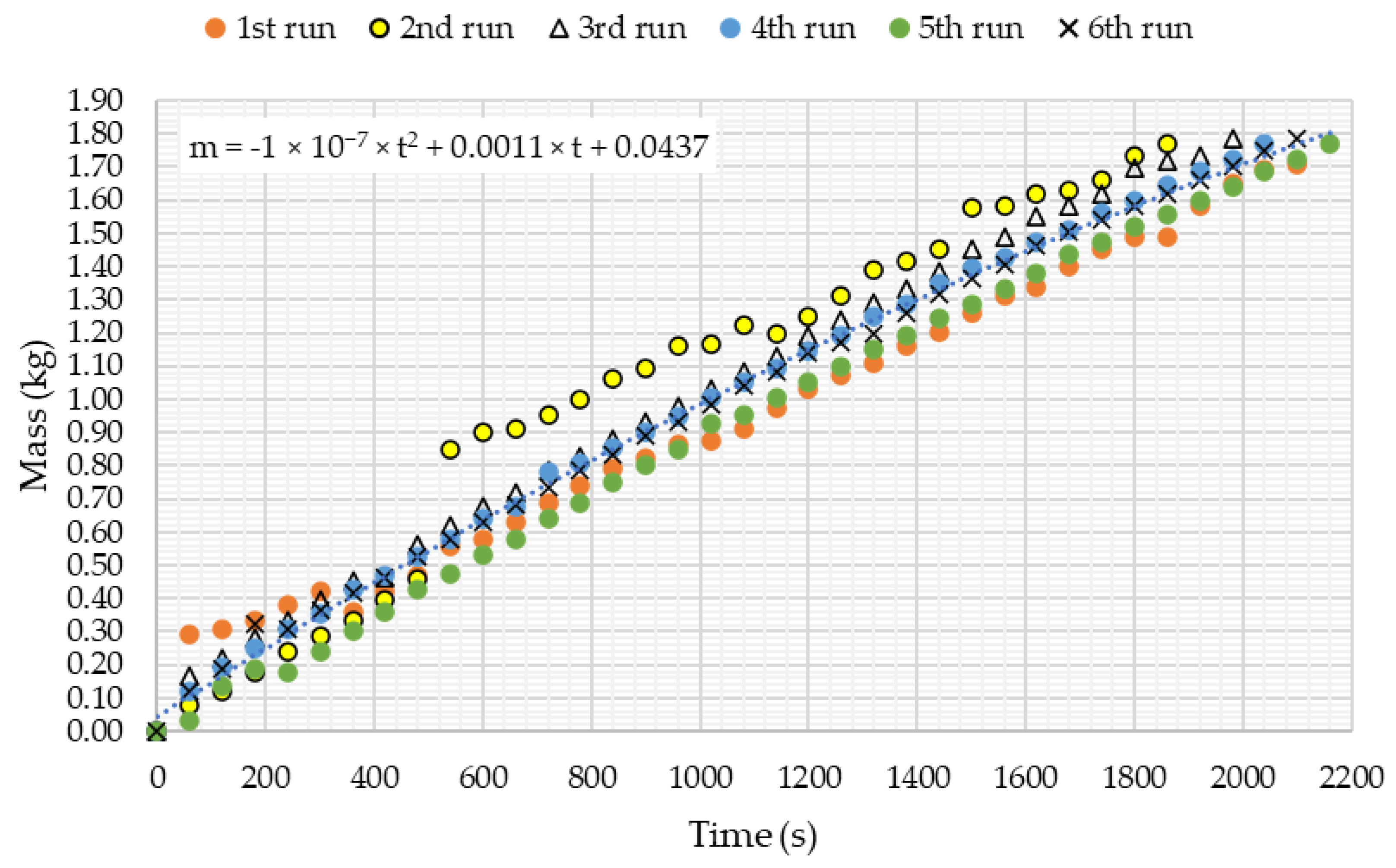
The average volumetric flow of raw biogas during all test runs was equal to 0.00097 m³/s, while an average mass flow was equal to 0.00087 kg/s. Both m₂(t) and V₁(t) dependencies were described as quadratic equations, which described a decrease of volumetric and mass flow of gas with an increase of pressure p₂.

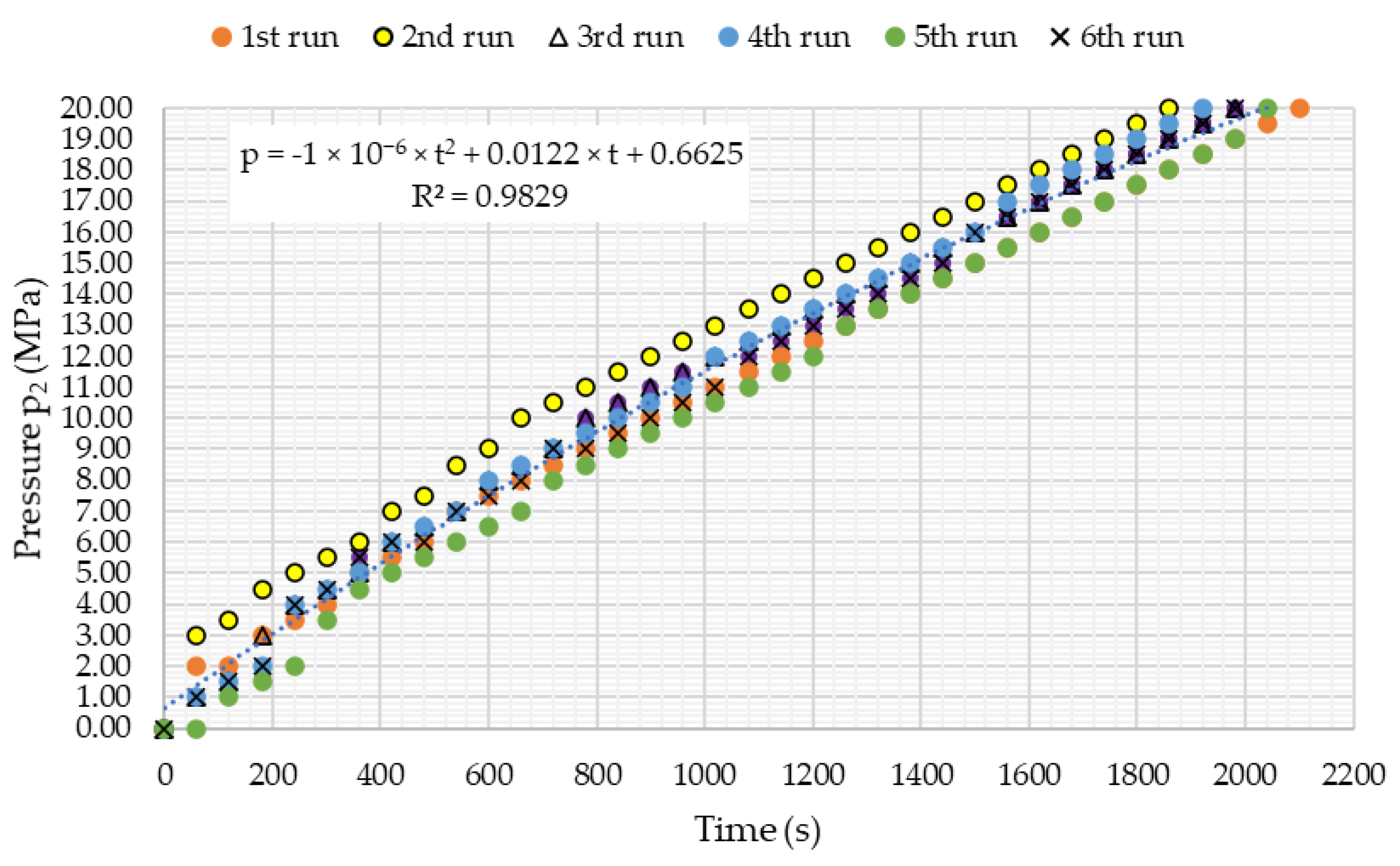
Figure 4 shows the measured volume of raw biogas in time for all test runs, and Figure 5 shows the measured mass of raw biogas in time. Figure 6 shows the measured pressure of raw biogas in the cylinder.

Data presented in Figure 4 and Figure 5 were used to derive equations describing the volume of gas stored in the cylinder and its mass in the function of compression time. Those equations, together with their domain and R² values, are presented in

Table 4. Equations for the determination of biogas volume and mass in compression.

Equation	R2	Domain
$V_1\left(t\right)=-9\times {10}^{-8}\times t^2+0.0015\times t-0.0078$	0.9989	$t\le 2160 \mathrm{s}$
$m_2\left(t\right)=-1\times {10}^{-7}\times t^2+0.0010541\times t+0.0437$	0.9728

.

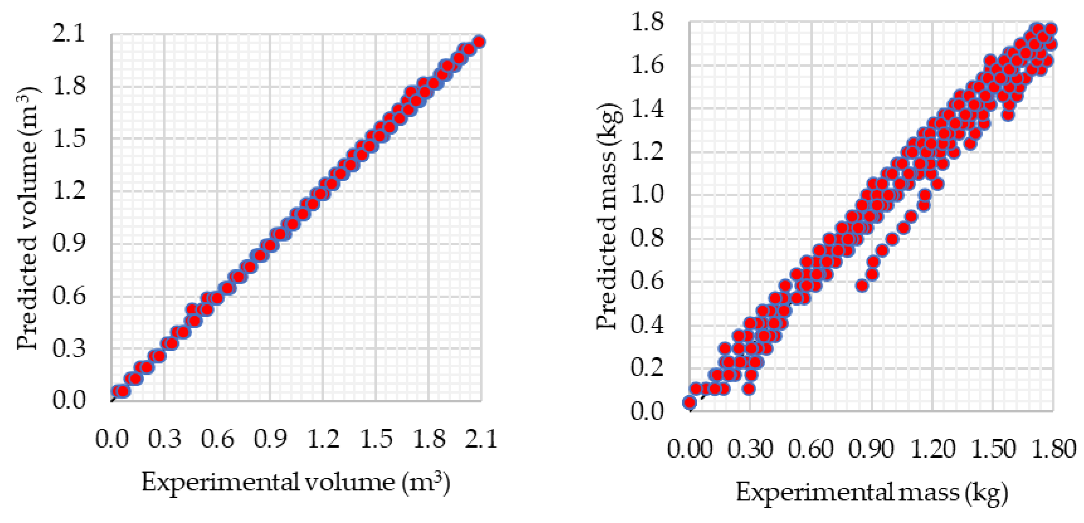
A comparison of experimental data with values predicted by equations shown in Table 4 is shown in Figure 7.

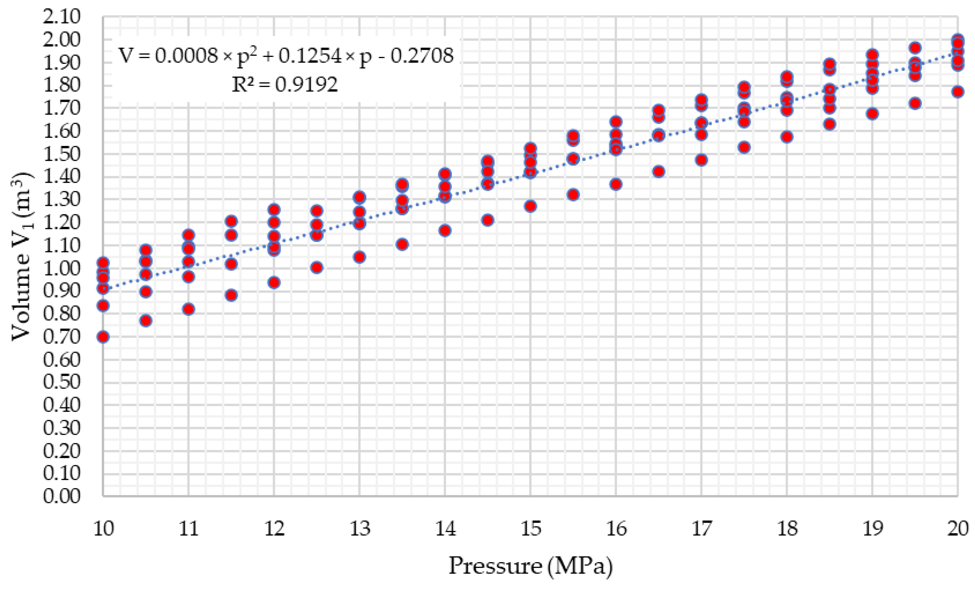
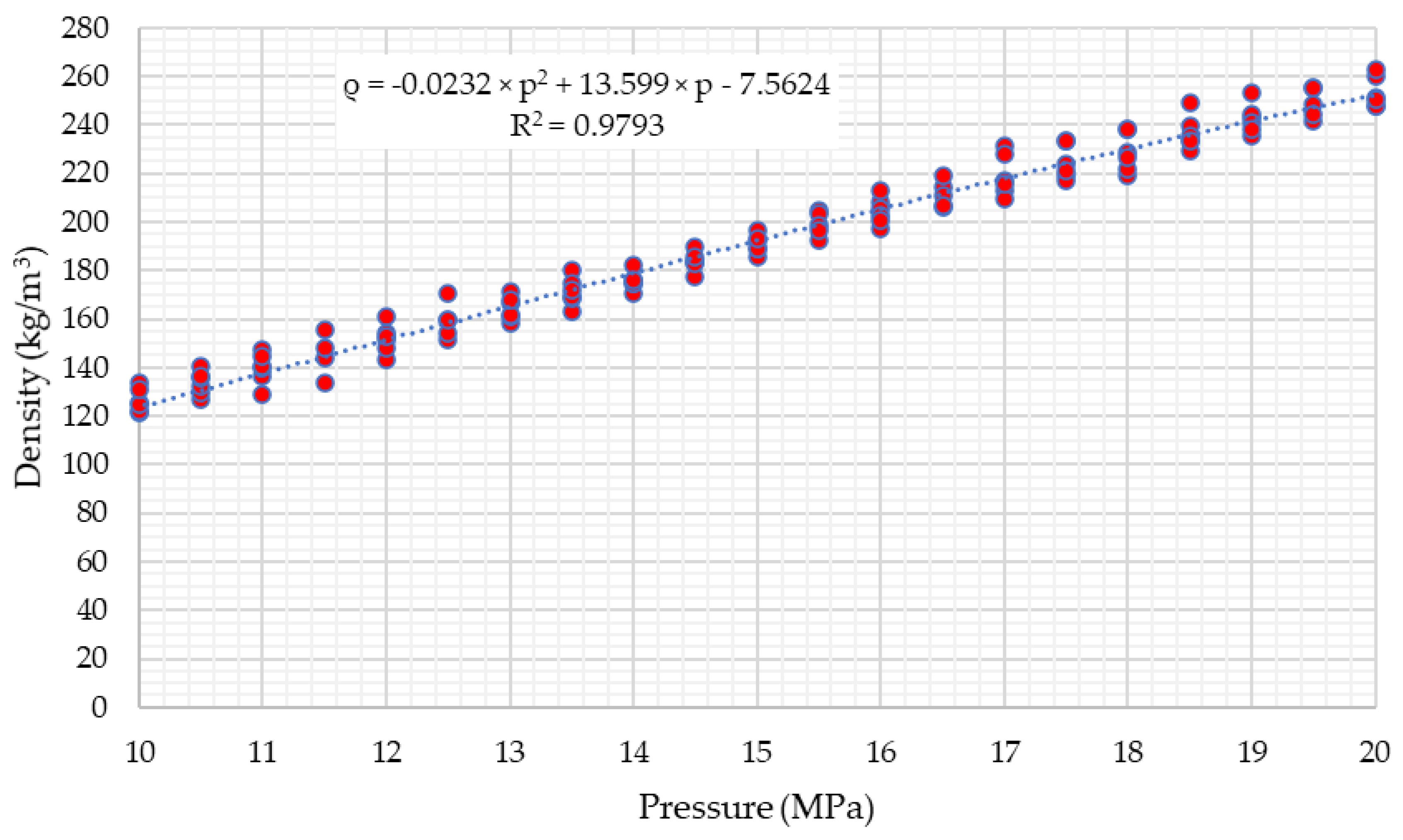
Figure 8 and Figure 9 show V₁(p₂) and ρ(p₂) dependences. For all 6 test runs, the biggest measured volume V₁ at p₂ = 20 MPa was equal to 2.04 m³, and the smallest was 1.77 m³. At p₂ = 10 MPa, measured values were in the range from 0.7 m³ to 1.03 m³.

3.2. Z-Factor Estimation

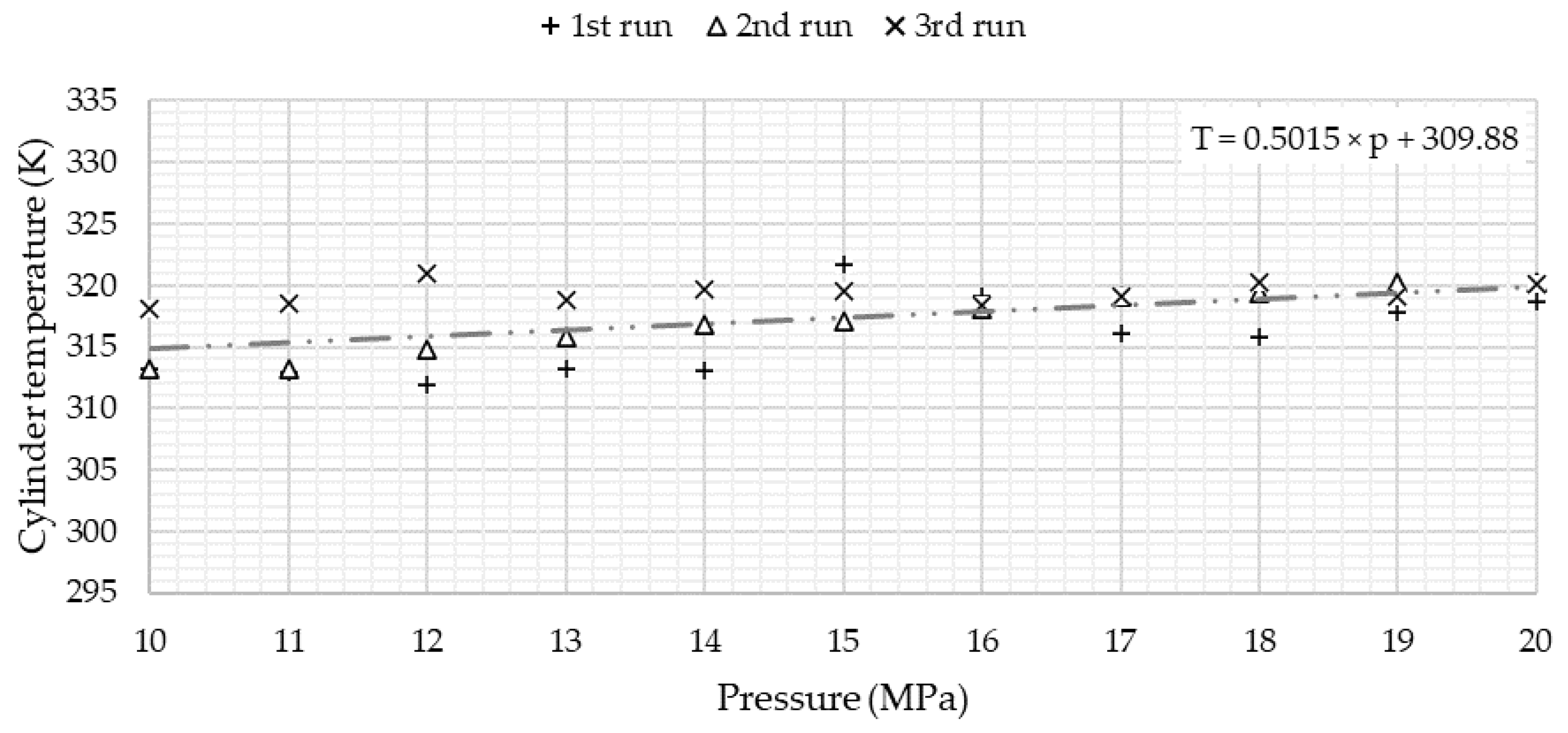
To obtain a comparable value of the compressibility factor of compressed raw biogas, linear regression was performed in order to determine T₂(p₂) dependence. The temperature was measured in the first three consecutive tests. T₂ values obtained using the approximation equation were compared with measured values to validate the approach. Validation was performed using a t-test for the expected value, which could be used only if the evaluated data followed a normal distribution. This was verified and confirmed by the Shapiro–Wilk test for normality of data distribution. Measured values of temperature are shown in

Table 5. Measured value of temperature at a given pressure.

Pressure	T2 1st Run	T2 2nd Run	T2 3rd Run	T2′ Linear appr.	Data Normality Test
					W Statistics	Critical Value
10	313.25	313.15	318.05	314.90	0.975	0.934
11	312.95	313.15	318.55	315.40
12	311.95	314.85	320.95	315.90
13	313.15	315.85	318.85	316.40	Data follow normal distribution
14	313.05	316.85	319.65	316.90	t-Test for Expected Value
15	321.75	317.15	319.55	317.40	H0: T2′ = T2
16	319.15	318.15	318.35	317.90	H0: T2′ < T2 v T2′ > T2
17	316.15	319.05	319.15	318.41	p-Value	No statistical reason to reject H0 hypotheses that T2′ = T2 at α = 0.05
18	315.85	319.45	320.25	318.91	0.990
19	317.75	320.25	319.15	319.41
20	318.65	320.25	320.15	319.91

, as well as the comparison between predicted and experimentally obtained values of T₂. Linear approximation of measured values of T₂ with respect to pressure p₂ is shown in Figure 10. The biggest measured temperature of the outer surface of the cylinder was equal to 320.25 K at p₂ = 18 MPa, the smallest being 311.95 K at p₂ = 12 MPa. The mean value of temperature was equal to 317.41 K.

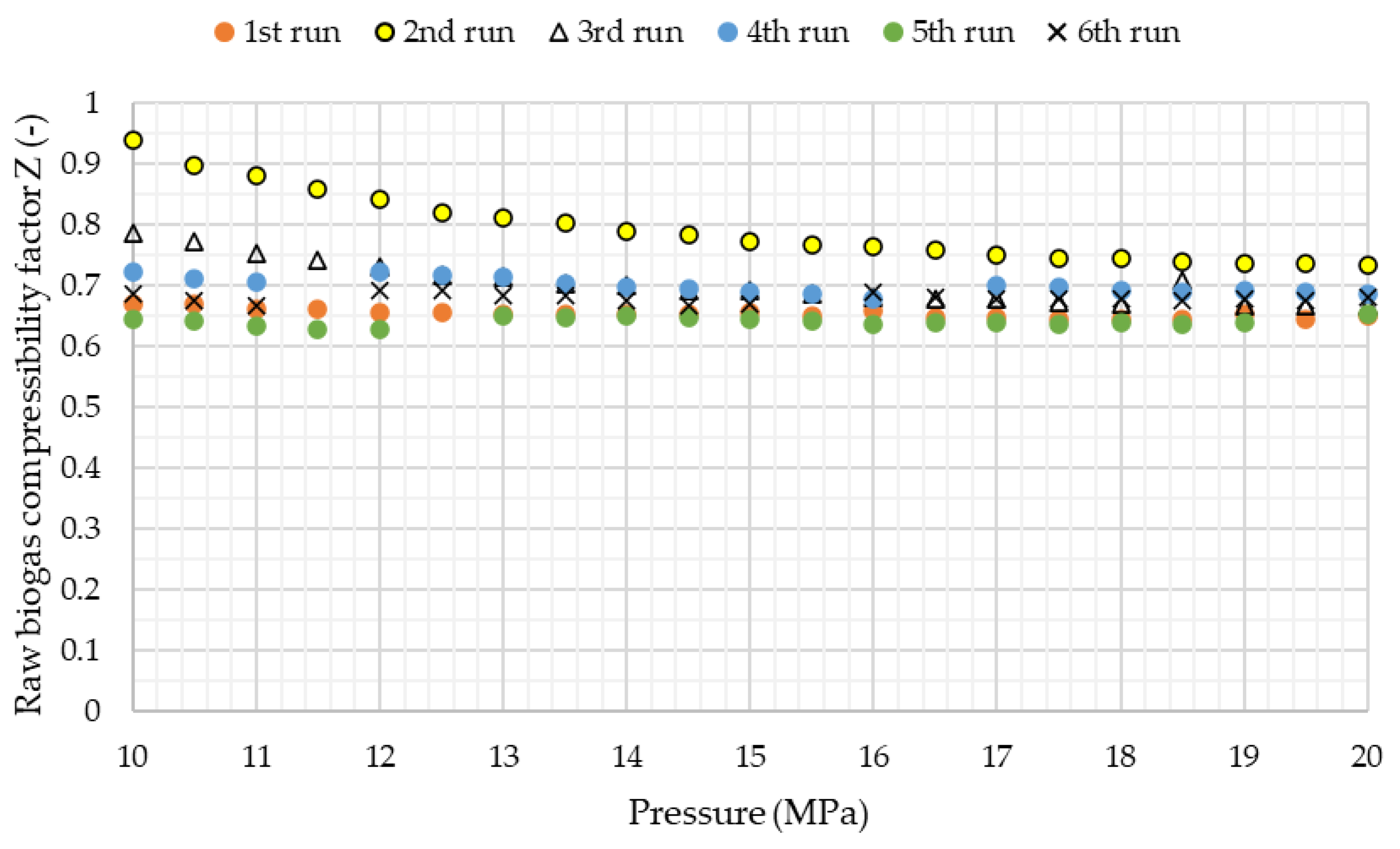
The calculated raw biogas compressibility factor based on obtained experimental results is shown in Figure 11. The largest obtained Z-factor based on experimental results was obtained for p₂ = 10 MPa and was equal to 0.908. The smallest was 0.608 at p₂ = 12 MPa. For p₂ equal to 20 MPa, compressibility factor Z was in the range from 0.62 (1st run) to 0.71 (2nd run).

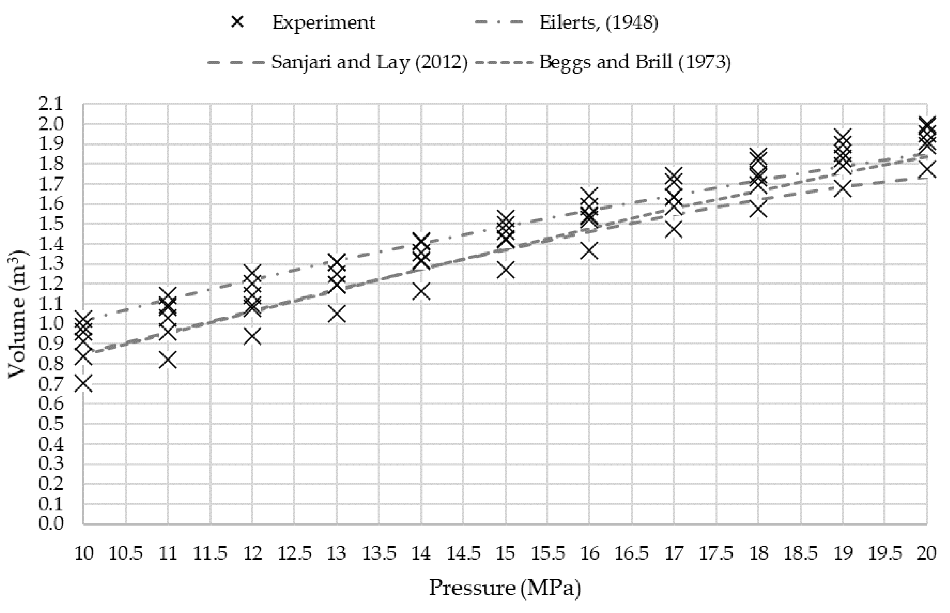
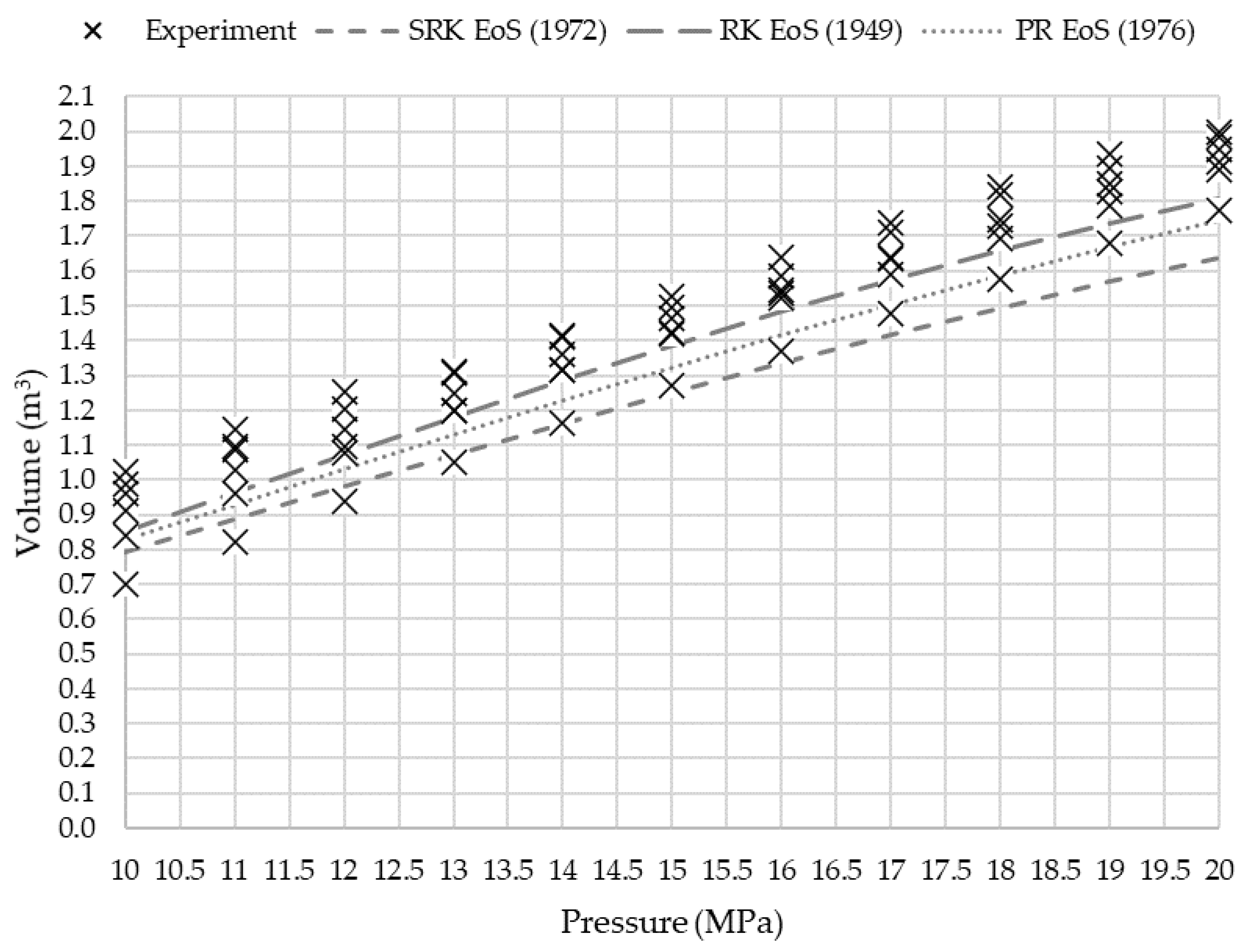
Measured values of V₁ were compared with values obtained using various equations of state and correlation methods, and results are shown in Figure 12 (EoS) and Figure 13 (correlation equations).

Results shown in Figure 12 and Figure 13 were compared using ARE%, AARE% and RMSE values for the entire dataset. Specific values are shown in

Table 6. Comparison of experimental results with numerical model predictions.

	RK EoS (1949)	SRK EoS (1972)	PR EoS (1976)	Eilerts, (1948)	Sanjari and Lay (2012)	Beggs and Brill (1973)
ARE%	−3.84	−12.60	−7.67	4.68	−5.20	−3.97
AARE%	7.22	13.44	9.60	7.21	8.14	7.26
RMSE	0.10	0.14	0.05	0.21	0.14	0.01

. The smallest value of AARE% was obtained for Eilerts (1948) and was equal to 7.21%, with the biggest value equal to 13.44% for SRK EoS (1972). The smallest value of RMSE equal to 0.01 was obtained for Beggs and Brill (1973), with the biggest value equal to 0.21 for Eilerts (1948).

Table 7. Comparison of biogas volume obtained from experimental results with numerical model predictions, p₂ = 20 MPa.

	Experiment		RK EoS (1949)	SRK EoS (1972)	PR EoS (1976)	Eilerts, (1948)	Sanjari and Lay (2012)	Beggs and Brill (1973)
Mean	1.918		1.809	1.637	1.745	1.852	1.736	1.838
Median	1.931	ARE%	−5.56	−14.52	−8.87	−3.30	−9.38	−4.02
Std dev	0.083	AARE%	6.25	14.52	8.87	4.81	9.38	5.27

shows the mean, median, and standard deviation of experimental results as well as ARE% and AARE% for numerical model validation for p₂ = 20 MPa, at temperature T₂′ = 319.9 K. The smallest value of AARE% was obtained for Eilerts (1948), and was equal to 4.81%, with the biggest value equal to 14.52% for SRK EoS (1972). The closest to 0 value of ARE% equal to −3.30% was obtained for Beggs and Brill (1973), with the biggest value equal to −14.52% for SRK EoS (1972).

3.3. Energy Balance for Raw Biogas Compression

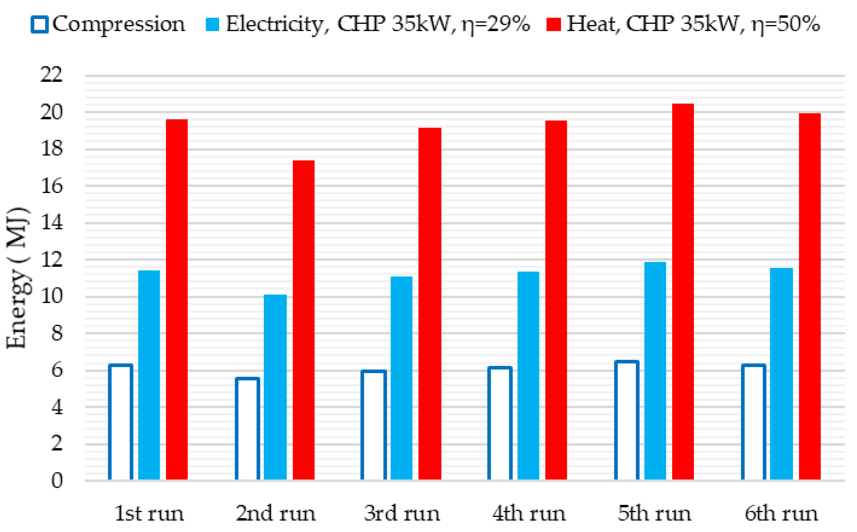
Figure 14 and Figure 15 show the theoretical amount of energy that can be obtained from biogas compressed in each of the 6 test runs for 2 CHP units (35 kW and 45 kW). The mean volume of compressed raw biogas V₁ was equal to 1.97 m³. Total energy content in biogas was equal to 38.71 MJ on average. Average compression time t_c was equal to 2040 s, during which an average of 6.12 MJ of electric energy was used.

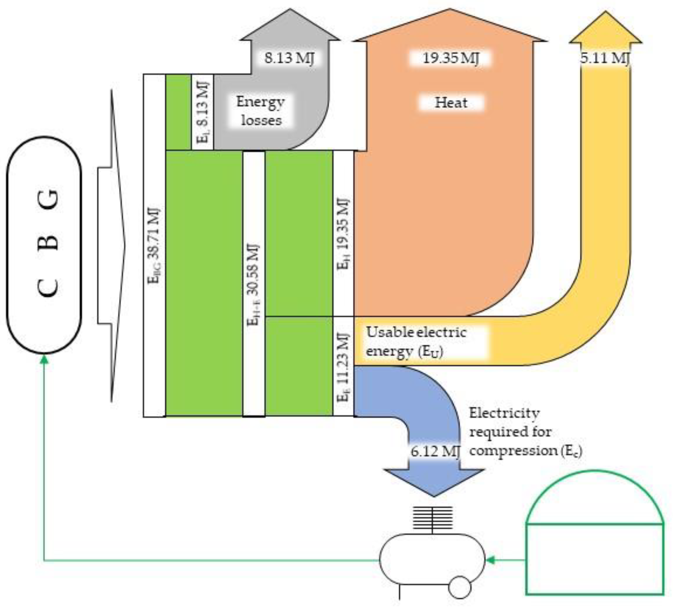
The Sankey diagram for the 35 kW CHP unit is shown in Figure 16. Data presented in the diagram correspond to the average energy content of compressed raw biogas. It was assumed that raw biogas stored in one cylinder of compressed biogas having a water volume of 0.0068 m³ and having a theoretical amount of energy E_BG = 38.71 MJ produces 19.35 MJ of heat (E_H) and 11.23 MJ of electricity (E_E) in CHP. To compress this amount of biogas, 6.12 MJ (E_c) of energy was used. It means, in a closed cycle from 38.71 MJ of the total energy stored in the cylinder (E_BG), 24.26 MJ can be used (E_H + E_U) on-site, providing that 6.12 MJ of electric energy (E_c) is being used for raw biogas compression in parallel to energy generation.

4. Discussion

The above results confirm findings published in [33] that raw biogas with CO₂ content greater than 40% can be compressed to a pressure equal to 20 MPa. The increased pressure of raw biogas during compression is reflected in the decrease of its compressibility factor Z. Measured values of volume of raw biogas in transport are consistent with theoretical predictions based on numerical models published elsewhere [19,20,25,26,27]. This is explained by the reduced spacing between molecules of the gas mixture inside the cylinder, which are of great importance in CH₄/CO₂ mixtures [34]. The pressure range covered in experimental research is in agreement with the typical storage conditions of CNG [1,4,22,30].

It was shown that methods based on fitting of S-K Chart are more suitable for estimation of compressibility factor for raw biogas. For pressure range between 10 MPa at 314.9 K and 20 MPa at 319.9 K, minimum values of ARE% were obtained for RK EoS (−3.84%) and Beggs and Brill fitting method (−3.97%). Maximum values ARE% were obtained for SRK EoS (−12.60%) and Sanjari and Lay fitting method (−5.20%). In terms of absolute average relative error (AARE%), minimum values were obtained for RK EoS (7.22%) and Eilert’s method (7.21%). The latter is very convenient as it provides a rapid estimation of raw biogas compressibility factor, similar to the study [32]. Maximum values of AARE% were obtained for SRK EoS (13.44%) and Sanjari and Lay (8.14%).

All theoretical models except SRK EoS predicted the final volume of raw biogas with CH₄/CO₂ content of 55%/44% stored in the cylinder with a water volume of 0.0068 m³ with an accuracy smaller than 10%. It was observed that experimentally obtained values of the Z-factor for raw biogas were higher than those predicted by numerical models based on obtained results. A possible reason for this discrepancy may be connected with an assumption that the temperature of the pressure vessel’s wall was equal to the temperature of compressed gas. According to Equation (5), the higher T₂, the smaller the Z-factor. For further investigation of the influence of gas temperature on its compressibility factor, additional research should be conducted in which isothermal conditions of compression would be assured.

Numerical models used in the study were more effective in the estimation of volume V₁ of raw biogas under pressure p₂ = 20 MPa than in the entire compression range. Minimum values of ARE% and AARE% were obtained for Eilerts method (ARE = −3.30%, AARE = 4.81%). The mean value of compressed biogas being the result of the experimental study was equal to 1.918 m³. The smallest predicted value was obtained for SRK EoS (1.637 m³), the biggest for Eilert’s method (1.852 m³). However, this value is much different from the value predicted by the ideal gas model, which is reflected in the gas compressibility factor, also called the gas deviation factor. For the mean value of the Z-factor determined experimentally, which was equal to 0.654, the predicted volume of gas stored in a given volume would be 34.5% smaller than the actual volume.

The measured density of raw biogas stored in the pressure vessel was in the range between 121.32 kg/m³ for p₂ = 10 MPa, T₂ = 313.25 K and 262.50 kg/m³ for p₂ = 20 MPa, T₂ = 320.15 K. Results are similar to other research for similar gas composition, temperature and pressure range [35], where measured values of density of the binary mixture of CH₄/CO₂ being 60%/40% were in the range between 141.056 kg/m³ for p₂ = 9.997 MPa, T₂ = 305.18 K and 283.653 kg/m³ for p₂ = 17.994 MPa, T₂ = 05.24 K. Experimentally determined density of compressed raw biogas makes it possible to estimate the mass of gas being stored in relation to its volume. This is of great importance when designing biogas distribution and storage systems, while this is one of the key parameters affecting materials selection and mechanical design of the system [4,30,32].

Mean value of the volume of raw biogas stored in the cylinder under a pressure of 20 MPa was equal to 1.97 m³ at a pressure of 20 MPa and temperature of 319.9 K. Assuming that the same pressure and temperature conditions would persist for systems having a bigger capacity for gas storage, it was possible to calculate the volume of raw biogas in transport for Mobile Biogas Station, as described in [4,30,32]. For ISO containers with a water capacity of 14.96 m³, for raw biogas characterized by Z-factor equal to 0.65, based on experimental results of this study, it is possible to estimate that the total volume of transported gas under pressure 20 MPa and temperature of 319.9 K would be equal to 3905.2 m³. Based on the measured value of raw biogas density, this amount of gas would have a mass of 3.751 kg, which is possible to be transported using road, rail and water transport. This value, when predicted by numerical models mentioned in this study, would differ by a maximum of −13.81%. Assuming CHP unit based on research [9] (case A), electric energy equal to 6178.5 MJ for CHP unit having 35 kW of power and 7030.7 MJ for CHP unit having 40 kW is possible to be generated. This amount, providing it could be properly stored and distributed, would be enough to power 3 residential dwellings in Poland for a year, assuming annual electricity consumption to be equal to 2003 kWh as published in [36].

Table 8. Electric energy possible to be obtained in CHP from compressed raw biogas.

	Z (-)	V1 (m3)	ERR (%)	E (kWh)	Eel 35 kW (kWh)	Eel 40 kW (kWh)
Experiment	0.65	3905.2		76,698.7	6178.5	7030.7
RK EoS (1949)	0.69	3718.6	−4.78%	73,033.1	5883.2	6694.7
SRK EoS	0.76	3365.8	−13.81%	66,105.1	5625.1	6059.6
PR EoS	0.71	3588.0	−8.12%	70,468.7	5676.6	6459.6
Beggs and Brill (1973)	0.68	3779.1	−3.23%	74,221.5	5979.0	6803.6
Sanjari and Lay	0.72	3548.2	−9.14%	69,685.8	5613.6	6387.9
Eilerts	0.67	3812.9	−2.36%	74,886.2	6032.5	6864.6

summarizes this data.

This study contributes to the development of biogas as an energy source that is ready to be supplied to remote areas by intermodal transport using modular gas containers. The novelty of findings with respect to existing publications in the field [8,9,10,11,12,13,30,32,37,38] is connected with experimental, on-site research on raw biogas compression that demonstrates the potential for application of this green energy source worldwide. The proposed method of biogas compression, combined with existing research and technical solutions on energy generation from raw biogas, can contribute to the effective development of circular economy and sustainable energy systems.

5. Conclusions

Results of performed experimental research on on-site raw biogas compression have provided significant and novel data regarding the volume of gas that can be stored under elevated pressure. Those results are of great importance in further research and development activities dedicated to energy supply systems, especially in rural areas, by increasing the diversity of gaseous fuels available on the market. It was shown that raw biogas can be compressed on-site to a pressure of 20 MPa and that widely known numerical models can predict the volume of compressed gas with an absolute average relative error as low as 4.81%. It means that those numerical models, especially fitting methods of Beggs and Brill and Sanjari and Lay, can be used for rapid estimation of raw biogas compressibility factor under given temperature and pressure providing that composition of biogas is known. Knowledge acquired in this study can be used by third parties to create development strategies based on an increasing area of energy supply, even to areas not connected to the gas grid.

Another important finding is that the density of compressed biogas at a pressure of 20 MPa equals 250.74 kg/m³. For 20 ft ISO containers with a storage volume of 14.96 m³, one transport of raw biogas would weigh 3751 kg. This information is of great importance when designing and optimizing gas storage units is considered.

The results presented in this study confirm the theoretical analysis of the raw biogas distribution network published in [4,30,32] and create new opportunities for biogas plants to utilize raw biogas more effectively by the implementation of biogas export in compressed form, increasing availability of renewable fuels and diversity of energy sources. Future work should involve experimental testing of isothermal compression of raw biogas to eliminate gas temperature influence and its measuring method on obtained results. The decompression process should also be investigated because compressed gas has some additional energy stored, manifested by increased pressure, that could be potentially utilized at recipients to increase the energy balance of compressed biogas systems. Additionally, presented results require expansion by experimental research on combustion of biogas supplied from pressurized vessels in the scope of the supply pressure, temperature and outflow of gas from the cylinder, as it is a very important aspect in the future design of biogas energy systems and can fully validate the efficiency of CBDS.

Obtained results confirm the potential of CBDS to increase renewable fuel availability (biogas) in remote areas and make it possible to reduce greenhouse emissions in the circular economy, and increased the share of renewables in electricity and heat generation. This concept creates a fundament for the development of green fuel and should be further investigated.